The document discusses consumer behavior, focusing on the study of individuals' purchasing patterns and the concept of utility, which measures consumer satisfaction derived from goods or services. It outlines key concepts such as total and marginal utility, the law of diminishing marginal utility, and various approaches to understanding consumer behavior, including cardinal and ordinal utility theories. Additionally, it introduces the concepts of indifference curves, budget lines, and the effects of income and price changes on consumer equilibrium.

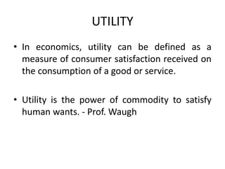
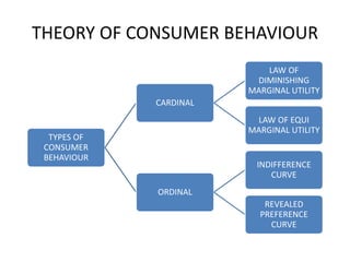
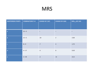
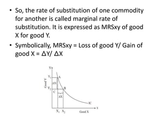
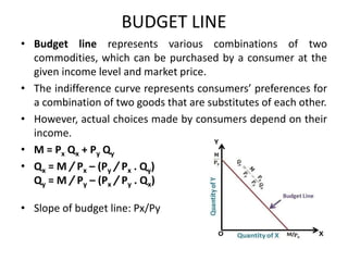
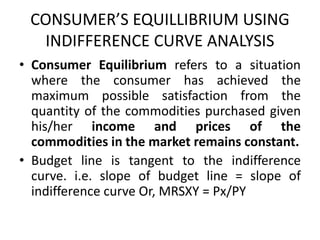
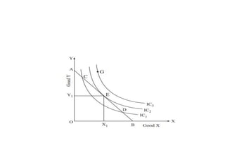
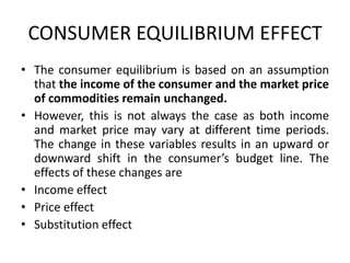
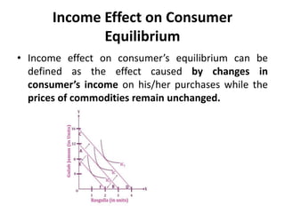
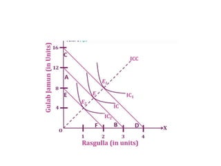
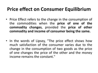
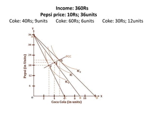
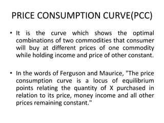
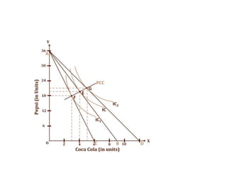
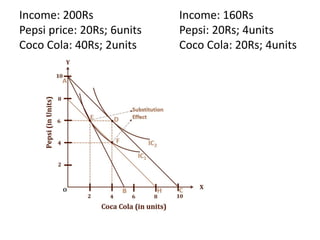
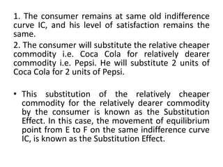
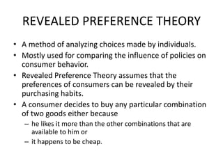
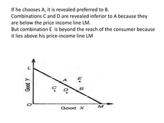
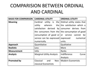
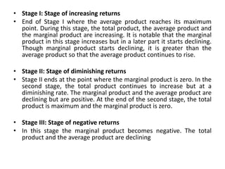
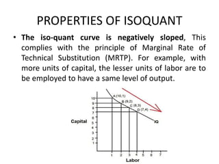
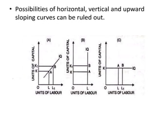
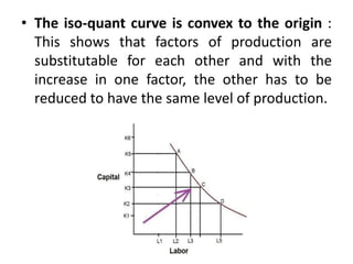
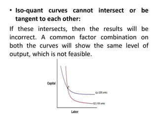
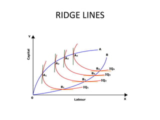
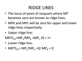
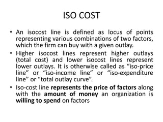
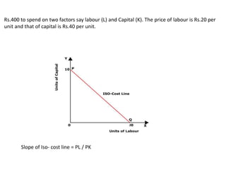
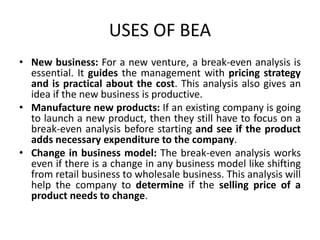
1. CONSUMER AND PRODUCER
BEHAVIOUR
MODULE 3

2. INRODUCTION TO CONSUMERS
BEHAVIOUR
• Consumer behavior is the study of individuals, groups, or
organizations and all the activities associated with the purchase,
use and disposal of goods and services.
• Consumer demand is defined as the willingness and ability of
consumers to purchase a quantity of goods and services in a given
period of time, or at a given point in time.
Consumers consider various factors before making purchases.
• Consumer demand analysis is a process of assessing consumer
behavior based on the satisfaction of wants and needs generated
by a consumer from the consumption of various goods.
• The satisfaction that consumers gain out of the consumption of a
commodity or service is called utility.

3. UTILITY
• In economics, utility can be defined as a
measure of consumer satisfaction received on
the consumption of a good or service.
• Utility is the power of commodity to satisfy
human wants. - Prof. Waugh

4. CONCEPTS OF UTILITY
• Total Utility
• Definition: Total utility is defined as the sum of the utility derived
by a consumer from the different units of a commodity or service
consumed at a given period of time.
• Assume that an individual consumes five units of a commodity X at
a given period of time and derives utility out of the consumption of
each unit as u1, u2, u3, u4, and u5.
The total utility is measured as follows:
TU = U1 + U2 + U3 + U4 + U5
• If the individual consumes n number of commodities, his/her total
utility, TUn, will be the sum of the utility derived from each
commodity. For example, an individual consumes commodities X, Y,
and Z and their respective utilities are Ux, Uy, and Uz, then total
utility is expressed as follows:
• TUn = Ux + Uy + Uz

5. CONCEPTS OF UTILITY
• Marginal Utility
• Definition: Marginal utility is defined as the utility derived from the
marginal or additional unit of a commodity consumed by an individual.
• It can also be defined as the addition to the total utility of a commodity
resulting from the consumption of an additional unit.
• Therefore, marginal utility, MU of a commodity X, is the change in the
total utility, ∆ TU, attained from the consumption of an additional unit of
commodity X.
Mathematically, it can be expressed as:
• MUx = ∆ TUx / ∆ Qx
• Where TUx = Total utility, ∆Qx = Change in quantity consumed by one
additional unit
• When total number of unit consumed is n, a marginal utility can also be
expressed as:
• MU of nth unit = TUn – TUn – 1

6. RELATION BETWEEN TOTAL AND
MARGINAL UTILITY

7. RELATION BETWEEN TOTAL AND
MARGINAL UTILITY

8. THEORY OF CONSUMER BEHAVIOUR
TYPES OF
CONSUMER
BEHAVIOUR
CARDINAL
LAW OF
DIMINISHING
MARGINAL UTILITY
LAW OF EQUI
MARGINAL UTILITY
ORDINAL
INDIFFERENCE
CURVE
REVEALED
PREFERENCE
CURVE

9. CARDINAL APPROACH
• Cardinal Utility explains that the satisfaction level after
consuming a good or service that can be scaled in terms of
countable numbers.
• The cardinal utility theory or approach was proposed by
classical economists, Gossen (Germany), William Stanley
Jevons (England), Leon Walras (France), and Karl Menger
(Austria).
• Later on a neo-classical economist, Alfred Marshall brought
about significant refinement in the cardinal utility theory.
Therefore, cardinal utility theory is also known as neo-
classical utility theory.

10. • Neo-classical economists believed that utility is
cardinal or quantitative like other mathematical
variables, such as height, weight, velocity, air
pressure, and temperature. They developed a
unit of measuring utility called utils.
• For example, according to the cardinal utility
concept, an individual gains 20 utils from a pizza
and 10 utils from coffee. In the measurement of
utility, neo-classicists assumed that one util
equals one unit of money and the utility of
money remains constant.

11. ASSUMPTONS OF CARDINAL
APPROACH

12. • Utility is measurable
• The basic assumption of the cardinal utility approach is that utilities of
commodities can be quantified. According to Marshall, money is used to
measure the utilities of commodities. This implies that the amount of
money that a customer is willing to pay for a particular commodity is a
measure of its utility.
• Marginal utility of money is constant
• The cardinal utility approach assumes that money must measure the same
amount of utility under all circumstances. To put simply, the utility derived
from each unit of money remains constant.
• Utilities are additive
• As per this assumption, the utility derived from various commodities
consumed by an individual can be added together to derive the total
utility. Suppose an individual consumes X1, X2, X3,….Xn units of commodity
X and derives U1, U2, U3,….Un utility respectively, the total utility that the
individual derives from n units of the commodity can be expressed as
follows:
• Un = U1(X1) + U2(X2) + … + Un (Xn)

13. • According to the cardinal utility approach, a consumer
reaches his/ her equilibrium when the last unit of his/her
money spent on each unit of the commodity yield the
same utility. Therefore, the consumer would spend his/her
money income on commodity X so long as:
• MUx > Px (MUm)
Where Px is the price of the commodity, MUx is the marginal
utility of the commodity and MUm is the marginal utility of
money.
• A utility maximizing consumer reaches the equilibrium
when:
• MUx = Px (MUm) or = 1

14. Consumption Price(Px) MUx (Utils) MUx(in
Rupee)
(1 Util= Re.1)
MUx/P
Difference Remarks
1 10 20 20 10 Mux > Px,
Consumer will
increase
consumption
2 10 16 16 6 Mux > Px,
Consumer will
increase
consumption
3 10 10 10 0 Mux = Px,
Consumer
Equilibrium
4 10 4 4 -6 Mux < Px,
Consumer will
decrease
consumption
5 10 0 0 -10 Mux < Px,
Consumer will
decrease
consumption

15. Consumer Equilibrium Cardinal Utility

16. PROBLEM
Given below is the marginal utility of apples and
mangoes. The price of each is Rs.5. The
consumer has Rs.40 to spend on mangoes and
apples. What quantity of apples and mangoes,
he should purchase?
Units Apples Mangoes
1 15 11
2 13 10
3 12 8
4 10 7
5 8 6
6 6 4

17. LAW OF DIMINISHING MARGINAL
UTILITY(LDMU)
• The law of diminishing marginal utility states
that as the quantity consumed of a commodity
continues to increase, the utility obtained from
each successive unit goes on diminishing,
assuming that the consumption of all other
commodities remains the same.
• To put simply, when an individual continues to
consume more and more units of a commodity
per unit of time, the utility that he/she obtains
from each successive unit continues to diminish.

18. • For example, the utility derived from the first glass of
water is high, but with successive glasses of water,
the utility would keep diminishing. The law of
diminishing marginal utility is applicable to all kinds
of goods such as consumer goods, durable goods,
and non-durable goods.

21. ASSUMPTIONS TO LDMU
• Rationality
The law of marginal utility assumes that a consumer is a rational being who
aims at maximizing his/her utility at the given income level and the market
price.
• Measurement of utility
The utility of a commodity can be measured using quantifiable standards like
a cup of tea, a bag of sugar, a pair of socks, etc.
• Constant marginal utility of money
The marginal utility of consumer’s income is constant.
• Homogeneity of commodity
The successive units of a commodity consumed are homogenous or identical
in shape, size, color, taste, quality, etc.
• Continuity
The consumption of successive units of a commodity should be continuous
without intervals.
• Ceteris paribus
Factors, such as the income, tastes and preferences of consumers; price of
related goods; etc. remain unchanged.

22. LAW OF EQUI MARGINAL
UTILITY(LEMU)
• Law of Equi-Marginal Utility
• This law is based on the principle of obtaining maximum
satisfaction from a limited income. It explains the behavior of a
consumer when he consumes more than one commodity.
• The law states that a consumer should spend his limited income on
different commodities in such a way that the last rupee spent on
each commodity yield him equal marginal utility in order to get
maximum satisfaction.
• Suppose there are different commodities like A, B, …, N. A
consumer will get the maximum satisfaction in the case of
equilibrium i.e.,
• MUA / PA = MUB / PB = … = MUN / PN

23. Unit MU(chocolate) MU(Chips) MU/P(chocolate) MU/P(Chips)
1 100 35
2 90 30
3 80 25
4 70 20
5 60 15
6 50 10
7 40 5

24. Unit MU(chocolate) MU(Chips) MU/P(chocolate) MU/P(Chips)
1 100 35 10 7
2 90 30 9 6
3 80 25 8 5
4 70 20 7 4
5 60 15 6 3
6 50 10 5 2
7 40 5 4 1

25. ASSUMPTIONS OF THE LEMU
• There is no change in the price of the goods or
services.
• The consumer has a fixed income.
• The marginal utility of money is constant.
• A consumer has perfect knowledge of utility.
• Consumer tries to have maximum satisfaction.
• The utility is measurable in cardinal terms.
• There are substitutes for goods.
• A consumer has many wants.

26. ORDINAL APPROACH
• Ordinal Utility explains that the satisfaction after
consuming a good or service cannot be scaled in
numbers; however, these things can be arranged
in the order of preference.
• According to the ordinal theory, utility is a
psychological phenomenon like happiness,
satisfaction, etc. It is highly subjective in nature
and varies across individuals. Therefore, it cannot
be measured in quantifiable terms

27. INDIFFERENCE CURVE
• An indifference curve is a curve that represents all
the combinations of goods that give the same satisfaction to the
consumer.
• Since all the combinations give the same amount of satisfaction,
the consumer prefers them equally. Hence the name indifference
curve. When these combinations are plotted on the graph, the
resulting curve is called indifference curve. This curve is also called
the iso-utility curve or equal utility curve
• Prof. Henderson and Prof. Quandt have defined, “The locus of all
commodity combinations from which a consumer derives the same
level of satisfaction forms an indifference curve.”

28. Combination Mangoes Oranges
A 1 14
B 2 9
C 3 6
D 4 4
E 5 2.5

29. ASSUMPTIONS OF INDIFFERENCE
CURVE
• Two commodities
It is assumed that the consumer has fixed amount of money, all of which is to be spent only on
two goods. It is also assumed that prices of both the commodities are constant.
• Non satiety
Satiety means saturation or maximum satisfaction. And, indifference curve theory assumes that
the consumer has not reached the point of satiety. It implies that the consumer still has the
willingness to consume more of both the goods. The consumer always tends to move to a higher
indifference curve seeking for higher satisfaction.
• Ordinal utility
According to this theory, utility is a psychological phenomenon and thus it is unquantifiable.
However, the theory assumes that a consumer can express utility in terms of rank. Consumer can
rank his/her preferences on the basis of satisfaction yielded from each combination of goods.
• Diminishing marginal rate of substitution
Marginal rate of substitution may be defined as the amount of a commodity that a consumer is
willing to trade off for another commodity, as long as the second commodity provides same level
of utility as the first one.
And, diminishing marginal rate of substitution states that the rate by which a person substitutes X
for Y diminishes more and more with each successive substitution of X for Y.

30. INDIFFERENCE MAP
• An Indifference Map is a set of Indifference Curves. It
depicts the complete picture of a consumer’s
preferences. higher indifference curve implies
a higher level of satisfaction

31. PROPERTIES OF INDIFFERENCE CURVE
• Indifference curve slope downwards to right

32. • Indifference curve is convex to the origin
• The concept of indifference curve is based on the
properties of diminishing marginal rate of substitution.
• According to diminishing marginal rate of substitution,
the rate of substitution of commodity X for Y decreases
more and more with each successive substitution of X for
Y.
• Also, two goods can never perfectly substitute each
other. Therefore, the rate of decrease in a commodity
cannot be equal to the rate of increase in another
commodity.

33. The rate of decrease in consumption of coffee is not the same as rate of
increase in consumption of cigarette. Similarly, rate of decrease in
consumption of coffee has gradually decreased even with constant increase in
consumption of cigarette.
Thus, indifference curve is always convex (neither concave nor straight).
Combination Cigarette Coffee
A 1 12
B 2 8
C 3 5
D 4 3
E 5 2

34. • Indifference curve cannot intersect each other
• Each indifference curve is a representation of
particular level of satisfaction.
• The level of satisfaction of consumer for any given
combination of two commodities is same for a
consumer throughout the curve. Thus, indifference
curves cannot intersect each other.

35. • Higher indifference curve represents higher
level of satisfaction

36. MARGINAL RATE OF SUBSTITUTION(MRS)
• Marginal rate of substitution (MRS) refers to the
rate at which one commodity can be substituted
for another commodity maintaining the same
level of satisfaction.
• The MRS for two substitute goods X and Y may be
defined as the quantity of commodity X required
to replace one unit of commodity Y (or quantity
of commodity Y required to replace one unit of X)
such that the utility derived from either
combinations remains the same.

37. MRS
INDIFFERENCE POINTS COMBINATIONS Y+X CHANGE IN Y (ΔY) CHANGE IN X (ΔX) MRSY,X (ΔY/ ΔX)
a 25 + 3 – – –
b 15 + 5 -10 2 -5.00
c 8 + 9 -7 4 -1.75
d 4 + 17 -4 8 -0.50
e 2 + 30 -2 13 -0.15

38. • So, the rate of substitution of one commodity
for another is called marginal rate of
substitution. It is expressed as MRSxy of good
X for good Y.
• Symbolically, MRSxy = Loss of good Y/ Gain of
good X = ⵠY/ ⵠX

39. BUDGET LINE
• Budget line represents various combinations of two
commodities, which can be purchased by a consumer at the
given income level and market price.
• The indifference curve represents consumers’ preferences for
a combination of two goods that are substitutes of each other.
• However, actual choices made by consumers depend on their
income.
• M = Px Qx + Py Qy
• Qx = M / Px – (Py / Px . Qy)
Qy = M / Py – (Px / Py . Qx)
• Slope of budget line: Px/Py

40. CONSUMER’S EQUILLIBRIUM USING
INDIFFERENCE CURVE ANALYSIS
• Consumer Equilibrium refers to a situation
where the consumer has achieved the
maximum possible satisfaction from the
quantity of the commodities purchased given
his/her income and prices of the
commodities in the market remains constant.
• Budget line is tangent to the indifference
curve. i.e. slope of budget line = slope of
indifference curve Or, MRSXY = Px/PY

42. CONSUMER EQUILIBRIUM EFFECT
• The consumer equilibrium is based on an assumption
that the income of the consumer and the market price
of commodities remain unchanged.
• However, this is not always the case as both income
and market price may vary at different time periods.
The change in these variables results in an upward or
downward shift in the consumer’s budget line. The
effects of these changes are
• Income effect
• Price effect
• Substitution effect

43. Income Effect on Consumer
Equilibrium
• Income effect on consumer’s equilibrium can be
defined as the effect caused by changes in
consumer’s income on his/her purchases while the
prices of commodities remain unchanged.

44. INCOME CONSUMPTION CURVE(ICC)
• It is the curve that shows equilibrium quantities
of two commodities that would be purchased by
the buyer at different levels of income, keeping
prices the same.
• In the words of Ferguson, The income
consumption curve is the curve which shows the
points of equilibrium resulting from various levels
of money income and constant prices."

46. Price effect on Consumer Equilibrium
• Price Effect refers to the change in the consumption of
the commodities when the price of one of the
commodity changes, provided the price of other
commodity and income of consumer being the same.
• In the words of Lipsey, "The price effect shows how
much satisfaction of the consumer varies due to the
change in the consumption of two goods as the price
of one changes the price of the other and the money
income remains the constant."

47. Income: 360Rs
Pepsi price: 10Rs; 36units
Coke: 40Rs; 9units Coke: 60Rs; 6units Coke: 30Rs; 12units

48. PRICE CONSUMPTION CURVE(PCC)
• It is the curve which shows the optimal
combinations of two commodities that consumer
will buy at different prices of one commodity
while holding income and price of other constant.
• In the words of Ferguson and Maurice, "The price
consumption curve is a locus of equilibrium
points relating the quantity of X purchased in
relation to its price, money income and all other
prices remaining constant."

50. Substitution effect on Consumer
Equilibrium
• Substitution effect refers to the change in quantity
demanded of a commodity by a consumer due to change in
its relative price, while the income of consumer remains
the same.
• The relative prices of commodities change. In such a case,
one commodity becomes more affordable than the other.
• If with the change in prices of commodities, the income of
the consumer changes in such a way that his real income
remains the same, then the consumer will switch to
substitute goods at cheaper prices. Consequently, It will
affect the purchasing pattern of the consumer, and this
effect is known as the Substitution Effect

52. Income: 200Rs Income: 160Rs
Pepsi price: 20Rs; 6units Pepsi: 20Rs; 4units
Coco Cola: 40Rs; 2units Coco Cola: 20Rs; 4units

53. 1. The consumer remains at same old indifference
curve IC, and his level of satisfaction remains the
same.
2. The consumer will substitute the relative cheaper
commodity i.e. Coca Cola for relatively dearer
commodity i.e. Pepsi. He will substitute 2 units of
Coca Cola for 2 units of Pepsi.
• This substitution of the relatively cheaper
commodity for the relatively dearer commodity
by the consumer is known as the Substitution
Effect. In this case, the movement of equilibrium
point from E to F on the same indifference curve
IC, is known as the Substitution Effect.

54. REVEALED PREFERENCE THEORY
• A method of analyzing choices made by individuals.
• Mostly used for comparing the influence of policies on
consumer behavior.
• Revealed Preference Theory assumes that the
preferences of consumers can be revealed by their
purchasing habits.
• A consumer decides to buy any particular combination
of two goods either because
– he likes it more than the other combinations that are
available to him or
– it happens to be cheap.

55. If he chooses A, it is revealed preferred to B.
Combinations С and D are revealed inferior to A because they
are below the price income line LM.
But combination E is beyond the reach of the consumer because
it lies above his price-income line LM

56. COMPARISION BETWEEN ORDINAL
AND CARDINAL
BASIS FOR COMPARISON CARDINAL UTILITY ORDINAL UTILITY
Meaning Cardinal utility is the
utility wherein the
satisfaction derived by
the consumers from the
consumption of good or
service can be expressed
numerically.
Ordinal utility states that
the satisfaction which a
consumer derives from
the consumption of good
or service cannot be
expressed numerical
units.
Approach Quantitative Qualitative
Realistic Less More
Measurement Utils Ranks
Analysis Marginal Utility Analysis Indifference Curve
Analysis
Promoted by Classical and Neo-
classical Economists
Modern Economists

57. CONSUMER SURPLUS
• Consumer Surplus = What a
consumer is ready to pay –
what he actually pays
• Assumptions:
• MU of money remains constant.
• No substitute for the commodity
• The expected price should be more than the
actual price.
• Income, taste and preference should remain
constant.
• P ∝ 1/CS

58. 1. The Total Utility of consuming a product is as
follows:
If the price is Rs.4, calculate consumer’s surplus
2.The following demand schedule is given:
Draw the demand curve and graphically
calculate consumer’s surplus if the price is Rs.3
Price 5 4 3 2 1 0
Quantity 0 2 4 6 8 10
Units 1 2 3 4 5 6
TU(Rs) 8 15 21 25 28 30

59. PRODUCTION
• Production in Economics is sometimes defined as the
creation of utility or the creation of wants – satisfying
goods’ and services.
• “If consuming means extracting utilities from,” says
Fraser, “producing means putting utility into.”
• In economics, Production is a process of transforming
tangible and intangible inputs into goods or services.
• Raw materials, land, labour and capital are the tangible
inputs, whereas ideas, information and knowledge are
the intangible inputs. These inputs are also known as
factors of production.

60. PRODUCTION
• Production in Economics can be defined as an
organised activity of transforming physical
inputs (resources) into outputs (finished
products), which will satisfy the products’
needs of the society.

61. FACTORS OF PRODUCTION
• Factors of Production in Economics are the inputs that are
used for producing the final output with the main aim of
earning an economic profit.
• Land, labour, capital and entrepreneur are the main factors
of production. Each and every factor is important and plays
a distinctive role in the organisation.
• Factors of Production are:
• Land
• Labour
• Capital
• Entrepreneur

62. PRODUCTION FUNCTION
• Production function can be defined as a
technological relationship between the physical
inputs (i.e., factors of production) and the
physical output of the organization.
• Output refers to the volume of goods produced.
Q = f (x1, x2, x 3….xn ) in which Q is the quantity
produced during a given period of time and x1,
x2, x3 ….xn are the quantities of different factors
used in production i.e. Land, Labour, Capital, raw
material etc...,

63. SHORT RUN PRODUCTION FUNCTION
• It refers to production in the short-run where
there are some fixed factors and variable
factors. In the short-run, production will
increase when more units of variable factors
are used with the fixed factor. Law of variable
proportion comes under Short run
production.

64. LONG RUN PRODUCTION FUNCTION
• It refers to production in the long-run where
all factors become variable. In the long-run,
production can be increased by increasing
units of all the factors simultaneously and in
the same proportion. Laws of returns to scale
comes under long run production function.

65. LAWS OF PRODUCTION
LAWS OF PRODUCTION
SHORT RUN
LAW OF VARIABLE
PROPORTION (ONE
VARIABLE INPUT)
LONG RUN
ISOQUANT ANALYSIS (TWO
VARIABLE INPUT)
RETURNS TO SCALE (ALL
VARIABLE INPUTS)

66. LAW OF PRODUCTION
• Describes the ways to increase the production
• The output(production) can be increased by
increasing input(factors)
Factors are of two types
• Fixed factors: Land, plant,
equipment/machinery
• Variables factors: Raw materials, labor

67. CONCEPTS OF PRODUCTION
• Total Product (TP): It refers to the total
volume of goods produced during a specific
period of time
• Average Product(AP): It refers to the total
product divided by total number of variables
factors i.e.., labour.
• Marginal Product (MP): Addition to total
product resulting from a unit increase in the
quantity of the variable factor.

68. LAW OF VARIABLE PROPORTION
• In the short run the level of production can be
changed by changing the variable factor
proportions.
• This law examines the production function
with one variable factor, keeping the others
constant.

69. ASSUMPTIONS
• Only one factor is variable while others are
constant
• All units of variable factors are homogeneous.
• There is no change in technology
• It is possible to vary the proportions in which
different inputs are combined
• The products are measured in physical units
ie., in quintals, tons, kilos etc.

70. PRODUCTON SCHEDULES
QUANTITY
OF FIXED
FACTOR
OUANTITY
OF
VARIABLE
FACTOR(
LABOUR)
TP AP MP
2 acre 1 2
2 acre 2 5
2 acre 3 9
2 acre 4 12
2 acre 5 14
2 acre 6 15
2 acre 7 15
2 acre 8 14

71. PRODUCTON SCHEDULES
QUANTITY
OF FIXED
FACTOR
OUANTITY
OF
VARIABLE
FACTOR(
LABOUR)
TP AP MP
2 acre 1 2 2 2 STAGE 1
2 acre 2 5 2.5 3
2 acre 3 9 3 4
2 acre 4 12 3 3
2 acre 5 14 2.8 2 STAGE 2
2 acre 6 15 2.5 1
2 acre 7 15 2.1 0
2 acre 8 14 1.75 -1 STAGE 3

73. • Stage I: Stage of increasing returns
• End of Stage I where the average product reaches its maximum
point. During this stage, the total product, the average product and
the marginal product are increasing. It is notable that the marginal
product in this stage increases but in a later part it starts declining.
Though marginal product starts declining, it is greater than the
average product so that the average product continues to rise.
• Stage II: Stage of diminishing returns
• Stage II ends at the point where the marginal product is zero. In the
second stage, the total product continues to increase but at a
diminishing rate. The marginal product and the average product are
declining but are positive. At the end of the second stage, the total
product is maximum and the marginal product is zero.
• Stage III: Stage of negative returns
• In this stage the marginal product becomes negative. The total
product and the average product are declining

74. Stage 1:
• TP increases at an increasing rate upto a point F
• MP also rises and is maximum at point F
• AP goes on rising
• After point F, TP rises but at a diminishing rate
• MP falls but is positive
• Stage 1 ends where AP reaches its highest
Stage 2:
• TP continues to increase at a diminishing rate, until it reaches its
maximum point
• Both MP and AP continuously fall during this stage.
• Stage ends when TP reaches its maximum point
Stage 3:
• TP declines
• MP is negative
• AP is diminishing

75. Problems
1. The table given below shows the MPP of a factor. It is also
known that TPP at zero employment is 0. Determine its TPP
and APP.
2. Following is known about a firm.
You are required to determine and explain the law applicable for
the changes in output due to change in the input. Also
determine the stages in total product.
Factor
Employment
1 2 3 4 5 6
MPP 40 44 36 32 28 12
Units of
labour
1 2 3 4 5 6
Total Output 50 110 150 180 180 150

76. Problems
3. Identify the different output levels which make the different
phases/stages of operation of the law of variable proportion
from the following data:
4. Following is known about a firm.
You are required to determine and explain the law applicable for
the changes in output due to change in the input. Also
determine the stages in total product.
Variable input 0 1 2 3 4 5
Total product 0 8 20 28 28 26
Units of
labour
1 2 3 4 5 6
Total Output 100 220 300 360 360 300

77. RETURNS TO SCALE
• Scale means “size”
Returns to scale means:
• What return(Output) is yield, when there is
change in all factors in same proportion
• Describes what happens to long run returns as
the scale (Size) of production increases
• This law states that,
• “when there are proportionate change in the
amount of inputs, the output also changes”

78. ASSUMPTIONS TO THE LAW
1. All the factors of production (such as land,
labour and capital) are variable but organization
is fixed
2. There is no change in technology
3. There is perfect competition in the market
4. Outputs or returns are measured in physical
quantities
5. The entire operation is only for long-run

79. Classified into 3 categories:
• Increasing return to scale
• Constant return to scale
• Decreasing return to scale

80. • Increasing returns to scale:
• It occurs when the increase in output is more
than proportional to increase in inputs. The
first stage starts from the point of origin and
continues till the marginal product is
maximum. For example, if all the inputs are
increased by 5%, the output increases by
more than 5% i.e. by 10%. In this case the
marginal product will be rising.

81. • Phase II: Constant returns to scale:
• It occurs when the increase in output is
proportional to increase in inputs. If we
increase all the factors (i.e. scale) in a given
proportion, the output will increase in the
same proportion i.e. a 5% increase in all the
factors will result in an equal proportion of 5%
increase in the output. Here the marginal
product is constant.

82. • Phase III: Decreasing returns to scale:
• It occurs when the increase in output is less
than proportional to the increase in inputs.
For example: if all the factors are increased by
5%, the output will increase by less than 5%
i.e. by 3%. In this phase marginal product will
be decreasing.

83. Labor Capital TP MP
2 1 8 8 Increasing
returns to scale
4 2 18 10
6 3 30 12
8 4 40 10 Constant
returns to scale
10 5 50 10
12 6 60 10
14 7 68 8 Decreasing
returns to scale
16 8 74 6
18 9 78 4

85. FACTORS AFFECTING
Increasing returns to scale
• Technical and Managerial Indivisibility:
Implies that there are certain inputs, such as machines and human resource,
used for the production process are available in a fixed amount. These inputs
cannot be divided to suit different level of production.
• Specialization:
It implies that high degree of specialization of man and machinery helps in
increasing the scale of production. The use of specialized labour and
machinery helps in increasing the productivity of labour and capital per unit.
• Concept of Dimensions:
According to the concept of dimensions, if the length and breadth of a room
increases, then its area gets more than doubled. For example, length of a
room increases from 15 to 30 and breadth increases from 10 to 20. This
implies that length and breadth, of room get doubled. In such a case, the area
of room increases from 150 (15 x 10) to 600 (30 × 20), which is more than
doubled.

86. FACTORS AFFECTING
Decreasing returns to scale
• Complexity of Management
Large scale of production creates the problem of lack of proper
management, larger bureaucracy, red tapism, lengthy chain of
communication and command between the top- management and
men on the production line.
• Entrepreneur is a Fixed Factor:
An increase in scale may come to a point where the abilities and skills
of the entrepreneur may be fully utilized. An increase in the scale
beyond this point may decrease the efficiency of the entrepreneur.
This gives rise to diseconomies of scale.
• Exhaustibility of Natural Resources:
Another factor responsible for the diminishing returns in some
activities is the limitation of natural sources.

87. ISO QUANTS
• The isoquant analysis helps to understand how
different combinations of two or more factors are
used to produce a given level of output.
• The term ISO implies equal and quant means
quantity or output.
• “An isoquant is a curve showing all possible
combinations of inputs physically capable of
producing a given level of output.”- Ferguson
• Isoquant curves are also called as equal product
curves or production indifference curves or iso
product curves.

88. ASSUMPTIONS
• It is assumed that only two factors are used to
produce a commodity
• Factors of production can be divided into small
parts
• Technique of production is constant
• The substitution between the two factors is
technically possible
• Under the given technique, factors of production
can be used with maximum efficiency Production
with two variable inputs

90. ISOQUANT MAP
• A number of isoquants depicting different levels
of output are known as isoquant map
• Higher isoquant represents higher level of output
than the lower one.

91. MARGINAL RATE OF TECHNICAL SUBSTITUTION
• Marginal rate of technical substitution indicates the rate at
which factors can be substituted at the margin without
altering the level of output.
• More precisely, marginal rate of technical substitution of
labour for capital may be defined as the number of units of
capital which can be replaced by one unit of labour, the level
of output remaining unchanged.

93. PROPERTIES OF ISOQUANT
• The iso-quant curve is negatively sloped, This
complies with the principle of Marginal Rate of
Technical Substitution (MRTP). For example, with
more units of capital, the lesser units of labor are to
be employed to have a same level of output.

94. • Possibilities of horizontal, vertical and upward
sloping curves can be ruled out.

95. • The iso-quant curve is convex to the origin :
This shows that factors of production are
substitutable for each other and with the
increase in one factor, the other has to be
reduced to have the same level of production.

96. • Iso-quant curves cannot intersect or be
tangent to each other:
If these intersects, then the results will be
incorrect. A common factor combination on
both the curves will show the same level of
output, which is not feasible.

97. • Upper iso-quant curves yield higher outputs
This is possible because, at a higher curve, more
factors of production are employed either the
capital or the labor, which results in more
production.

98. EXCEPTIONS TO NORMAL SHAPE OF
ISOQUANT CURVE
• Linear Isoquant- When the two factors are perfect
substitutes for each other, then isoquants are straight lines
with negative slope. Marginal rate of technical substitution
between two perfect substitutes remains constant i.e. for
every addition in one factor, equal amount of other factor is
sacrificed.

99. EXCEPTIONS TO NORMAL SHAPE OF
ISOQUANT CURVE
• L Shaped Isoquants- Isoquants are L-Shaped or right angled in
case two factors are perfect complements. A producer can
increase the output by increasing the amount of both factors
proportionately. There will be no change in the level of output
if we change the quantity of one factor without changing the
quantity of other factor.

100. DIFFERENCE BETWEEN ISOQUANT
AND INDIFFERENCE CURVE

101. RIDGE LINES

102. RIDGE LINES
• The locus of point of isoquant where MP
becomes zero are known as ridge lines.
• MPK and MPL will be zero for upper and lower
ridge lines respectively.
• Upper ridge line:
MRTSLK=MPL/MPK =MPL /0 = ∞
• Lower ridge line:
• MRTSLK= MPL/MPK =0/ MPK = 0

103. ISO COST
• An isocost line is defined as locus of points
representing various combinations of two factors,
which the firm can buy with a given outlay.
• Higher isocost lines represent higher outlays
(total cost) and lower isocost lines represent
lower outlays. It is otherwise called as “iso-price
line” or “iso-income line” or “iso-expenditure
line” or “total outlay curve”.
• Iso-cost line represents the price of factors along
with the amount of money an organization is
willing to spend on factors

104. Rs.400 to spend on two factors say labour (L) and Capital (K). The price of labour is Rs.20 per
unit and that of capital is Rs.40 per unit.
Slope of Iso- cost line = PL / PK

105. PRODUCER’S EQUILLIBRIUM
POSITION THROUGH ISOQUANTS
• The basic objective of rational producer is to maximize
his profits and produces a given quantity of output
with that combination of factors that is ‘OPTIMUM’.
The optimum combination of resources is that
(1) Which minimize the cost of production for producing a
given level of output.
(2) Which produce maximum level of output for a given cost
of production.
• Thus, there are 2 cases of producer’s equilibrium:
1. Minimization of cost subject to an output constraint.
2. Maximization of output subject to a cost constraint.

106. CONDITIONS FOR EQUILLIBRIUM
• At the point of equilibrium ‘e’, slope of isoquant
and slope of iso-cost line is equal. Thus, the
conditions of producer’s equilibrium are:
1. Slope of isoquant = Slope of iso-cost line
MRTSLK= PL / PK
MPL / MPK = PL / PK
MPL / PL = MPK / PK
2. Isoquants must be convex to the origin

107. Minimization of cost subject to an
output constraint
• A single isoquant IQ showing output
constraint
• A series of iso-cost lines. Higher iso-cost line
represents higher money outlay. All iso-cost
lines are parallel to one another because
slope of all iso-cost line is same as the factor
prices remains constant
• The producer will be at equilibrium where
the given isoquant is tangent to the lowest
possible iso-cost line.

108. Maximization of output subject to a
cost constraint
• An iso-cost line PQ showing cost constraint.
• A series of isoquants. Higher isoquant shows
higher level of output.
• The producer equilibrium will be at the point
where the given iso-cost line is tangent to
the highest possible isoquant.

109. COST FUNCTION
• TC=TFC+TVC
• AC=TC/Q ; AFC= FC/Q; AVC= VC/Q
• MC = TCn- TCn-1 (or) VCn- VCn-1

110. ANALYSIS OF COST
• Money Cost : Money cost or nominal cost is
the total money expenses incurred by a firm in
producing a commodity. It includes: cost of
raw materials, payment of wages and salaries
payment of rent, interest on capital, expenses
on fuel and power, expenses on transportation
and so on.

111. ECONOMIES AND DISECONOMIES OF
SCALE
• Economies of scale, As a firm expands its
production capacity, the efficiency of production
also increases. It is able to draw more output per
unit of input, leading to low average total costs.
This condition is termed as economies of scale.
• Economies of scale result in cost-saving for a firm
as the same level of inputs yields a higher level of
output. A higher level of output results in lower
average costs as the total costs are shared over
the increased output.

112. ECONOMIES AND DISECONOMIES OF
SCALE
• Economies of scale, As a firm expands its production capacity, the
efficiency of production also increases. It is able to draw more
output per unit of input, leading to low average total costs. This
condition is termed as economies of scale.
• Economies of scale result in cost-saving for a firm as the same level
of inputs yields a higher level of output. A higher level of output
results in lower average costs as the total costs are shared over the
increased output.
• Diseconomies of scale refer to the disadvantages that arise due to
the expansion of a firm’s capacity leading to a rise in the average
cost of production.

113. ECONOMIES OF SCALE
• Internal economies of scale: Internal Economies of
Scale refers to the economies that a firm achieves due
to the growth of the firm itself. When an organization
reduces costs and increases the production, internal
economies of scale are achieved.
• Bulk-buying economies
• Technical economies
• Financial economies
• Marketing economies
• Managerial economies

114. • Bulk-buying economies: As a firm grows in size, it requires larger
quantities of production inputs, such as raw materials. With
increase in the order size, the firm attains bargaining power over
the suppliers. It is able to purchase inputs at a discount, which
results in lower average cost of production.
• Technical economies: As a firm increases its scale of production, it
may use advanced machinery or better techniques for production
purposes.
• For example, the firm may use mass-production techniques, which
provide a more efficient form of production. Similarly, a bigger firm
may invest in research and development to increase the efficiency
of production.
• Financial economies: Often small businesses are perceived as being
riskier than larger businesses that develop a credible track record.
Therefore, while the smaller firms find it hard to obtain finance at
reasonable interest rates, larger firms easily find potential lenders
to raise money at lower interest rates. This capital is further used
to expand the production scale resulting in low average total costs.

115. • Marketing economies: The marketing function of a firm
incurs a certain cost, such as costs involved in advertising
and promotion, hiring sales agents, etc. Many of these
costs are fixed and as the firm expands its capacity, it is able
to spread the marketing costs over a wider range of
products. This results in low-average total costs.
• Managerial economies: As a firm grows, managerial
activities become more specialized. For example, a larger
firm can further divide its management into smaller
departments that specialize in specific areas of business.
Specialist managers are likely to be more efficient as they
possess a high level of expertise, experience and
qualifications. This reduces the managerial costs in
proportion to the scale of production in the firm. Therefore,
economies of scale can be achieved with efficient
management.

116. • External economies of scale refer to the economies in
production that a firm achieves due to the growth of
the overall industry in which the firm operates.
External economies of scale transpire outside a firm,
within an industry. Therefore, when an industry’s scope
of operations expands, external economies of scale are
said to have been achieved.
• Factors of external economies of scale
• Improvement in transport and communication network
• Focus on training and education within the industry
• Support of other industries

117. DISECONOMIES OF SCALE
• There are two types of economies of scale:
– Internal diseconomies
– External diseconomies
• Internal diseconomies
• Internal diseconomies refer to the
diseconomies that a firm incurs due to the
growth of the firm itself.

118. Type of Internal diseconomies
• Managerial inefficiency: Often due to the challenge of managing a
bigger firm, managerial responsibilities are delegated to the lower
level personnel. As these personnel may lack the required
experience to undertake the challenge, it may result in low output
at a higher cost.
• Labour inefficiency: When a firm expands its production capacity,
work areas may become more crowded leaving little space for each
worker to work efficiently.
• Moreover, over-specialisation and division of labour in a bigger
firm create over-dependence on workers. In such situations, labour
absenteeism, lethargy, discontinuation of services, etc., become
common, which increase the long-run average cost of production.

119. External diseconomies of scale
• External diseconomies of scale refer to the disadvantages that arise due to an
increase in the number of firms in an industry-leading to overproduction.
• Factors of external diseconomies of scale
• increases the demand for raw materials. This leads to an increase in the prices of
raw materials consequently increasing the cost of production in the industry.
• increases the demand for skilled labour. This leads to an increase in the wages of
the skilled workers consequently increasing the cost of production in the industry.
• lead to problems of waste disposal. Firms are bound to employ expensive waste
disposal or recycling methods, which increases the long-run cost of production.
• The concentration of firms within an industry may lead to excessive need for
advertising and promotion, consequently increasing the cost of production in the
industry.

120. BREAK EVEN ANALYSIS
• A break-even analysis is an economic tool that is used
to determine the cost structure of a company or the
number of units that need to be sold to cover the cost.
Break-even is a circumstance where a company neither
makes a profit nor loss but recovers all the money
spent.
• The break-even analysis is used to examine the relation
between the fixed cost, variable cost, and revenue.
Usually, an organization with a low fixed cost will have
a low break-even point of sale.

121. ASSUMPTIONS
• (i) The total costs may be classified into fixed and variable costs. It
ignores semi-variable cost.
• (ii) The cost and revenue functions remain linear.
• (iii) The price of the product is assumed to be constant.
• (iv) The volume of sales and volume of production are equal.
• (v)The fixed costs remain constant over the volume under
consideration.
• (vi) It assumes constant rate of increase in variable cost.
• (vii) It assumes constant technology and no improvement in labour
efficiency.
• (ix) The factor price remains unaltered.
• (x) Changes in input prices are ruled out.
• (xi) In the case of multi-product firm, the product mix is stable.

122. DETERMINANTS OF BEA
• Fixed costs: These costs are also known as
overhead costs. These costs materialize once the
financial activity of a business starts. The fixed
prices include taxes, salaries, rents, depreciation
cost, labour cost, interests, energy cost, etc.
• Variable costs: These costs fluctuate and will
decrease or increase according to the volume of
the production. These costs include packaging
cost, cost of raw material, fuel, and other
materials related to production.

123. LIMITATIONS
• Doesn’t predict demand – Although a break-even analysis can
tell you when you’ll break even, it doesn’t give you any
insight into how likely that is to happen. Also, demand isn’t
stable, so even if you think there’s a gap in the market, your
break-even point could end up being a lot more ambitious
than you initially thought.
• Depends on reliable data – In short, the accuracy of your
break-even analysis is dependent on the accuracy of your
data. If your calculations are wrong or you’re dealing with
fluctuating costs, break-even analysis may not be the most
useful tool in your arsenal.

124. LIMITATIONS
• Too simple – Break-even analysis is best for companies with
one price-point. If you have multiple products with multiple
prices, then break-even analysis may be too simple for your
needs. In addition, it’s worth remembering that costs can
change, so your break-even point may need to be evaluated
and adjusted at a later time.
• Ignores competition – Another limitation of a break-even
analysis concerns the fact that competitors aren’t factored
into the equation. New entrants to the market could affect
demand for your products or cause you to change your
prices, which is likely to affect your break-even point.

125. USES OF BEA
• New business: For a new venture, a break-even analysis is
essential. It guides the management with pricing strategy
and is practical about the cost. This analysis also gives an
idea if the new business is productive.
• Manufacture new products: If an existing company is going
to launch a new product, then they still have to focus on a
break-even analysis before starting and see if the product
adds necessary expenditure to the company.
• Change in business model: The break-even analysis works
even if there is a change in any business model like shifting
from retail business to wholesale business. This analysis will
help the company to determine if the selling price of a
product needs to change.

126. • Break-even point = Fixed cost/-Price per cost
– Variable cost
• Example of break-even analysis
• Company X sells a pen. The company first
determined the fixed costs, which include a
lease, property tax, and salaries. They sum up
to ₹1,00,000. The variable cost linked with
manufacturing one pen is ₹2 per unit. So, the
pen is sold at a premium price of ₹10.

127. • Break-even point = Fixed cost/Price per cost –
Variable cost
• = ₹1,00,000/(₹12 – ₹2)
• = 1,00,000/10
• = 10,000
• Therefore, given the variable costs, fixed costs,
and selling price of the pen, company X would
need to sell 10,000 units of pens to break-
even.

128. RELATION BETWEEN AC AND MC

129. SHORT RUN

130. LONG RUN

131. RELATION BETWEEN PRODUCTION
AND COST