Downloaded 25 times


![Wi – Fi [IEEE 802.11]
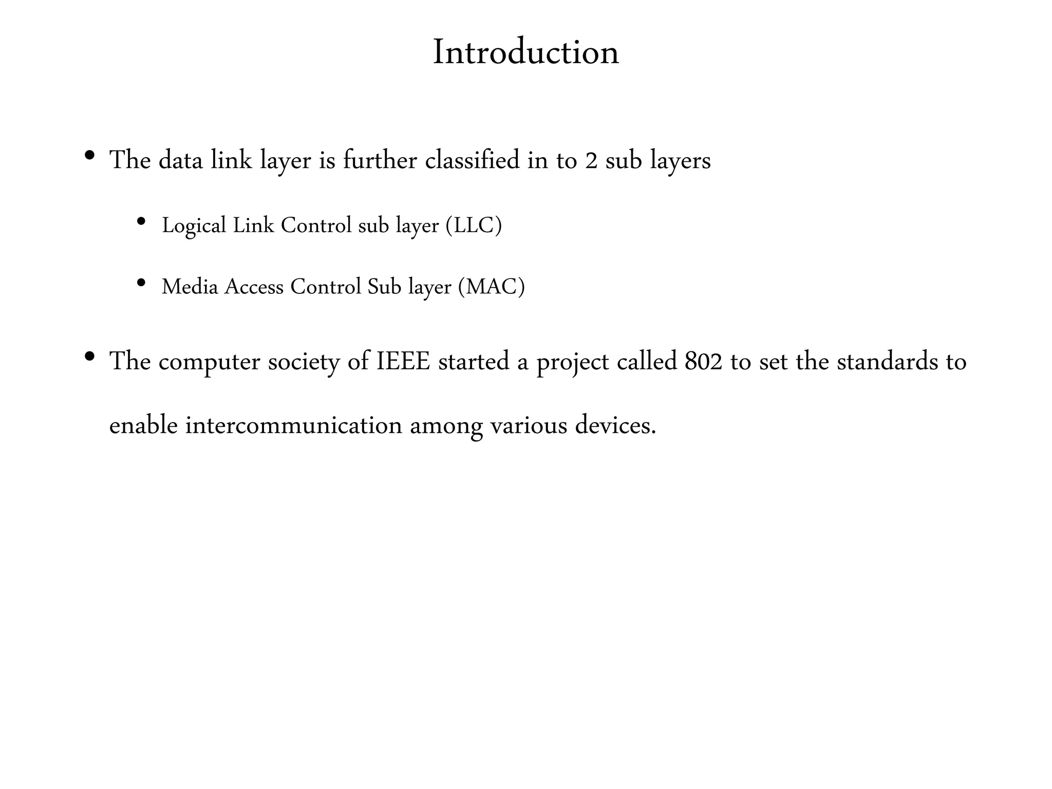
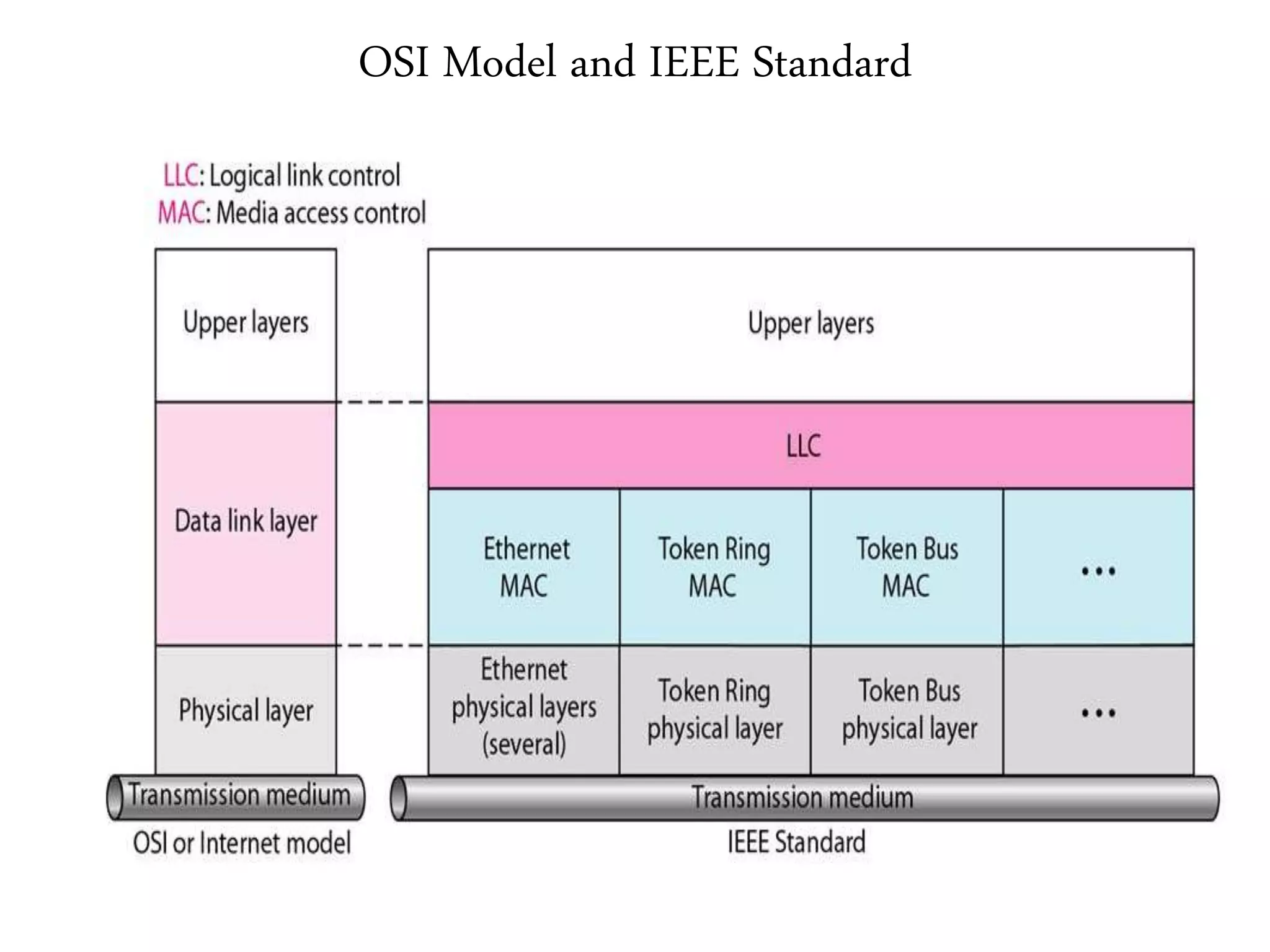
• IEEE 802.11 standards are designed for limited geographical area (Homes, Offices, Colleges
etc.,)
• We are about to discuss
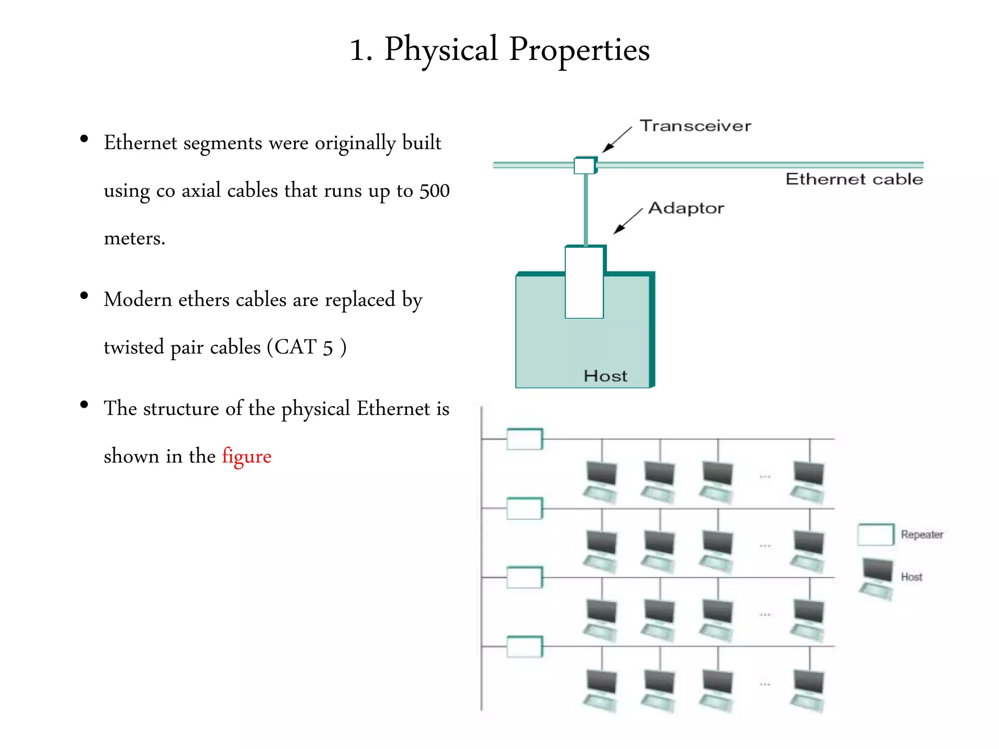
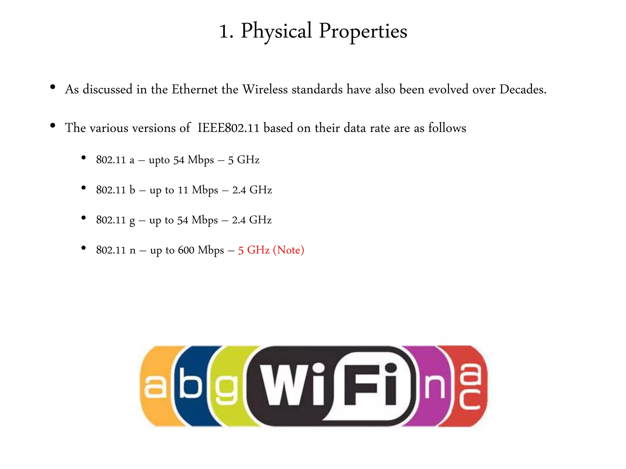
• Physical Properties – (Evolution)
• Problems in Wireless LAN’s
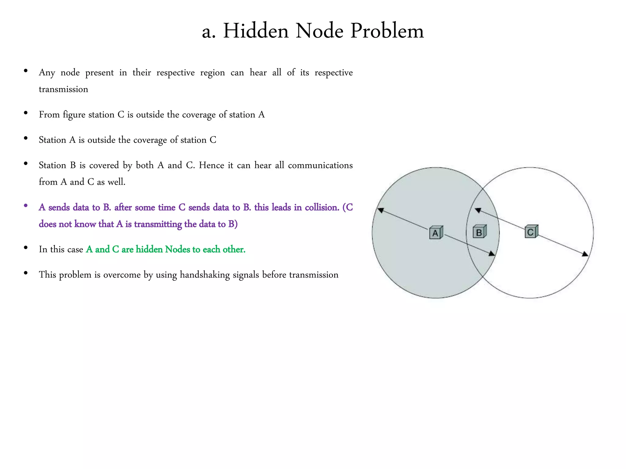
• Hidden Node Problem
• Exposed Node Problem
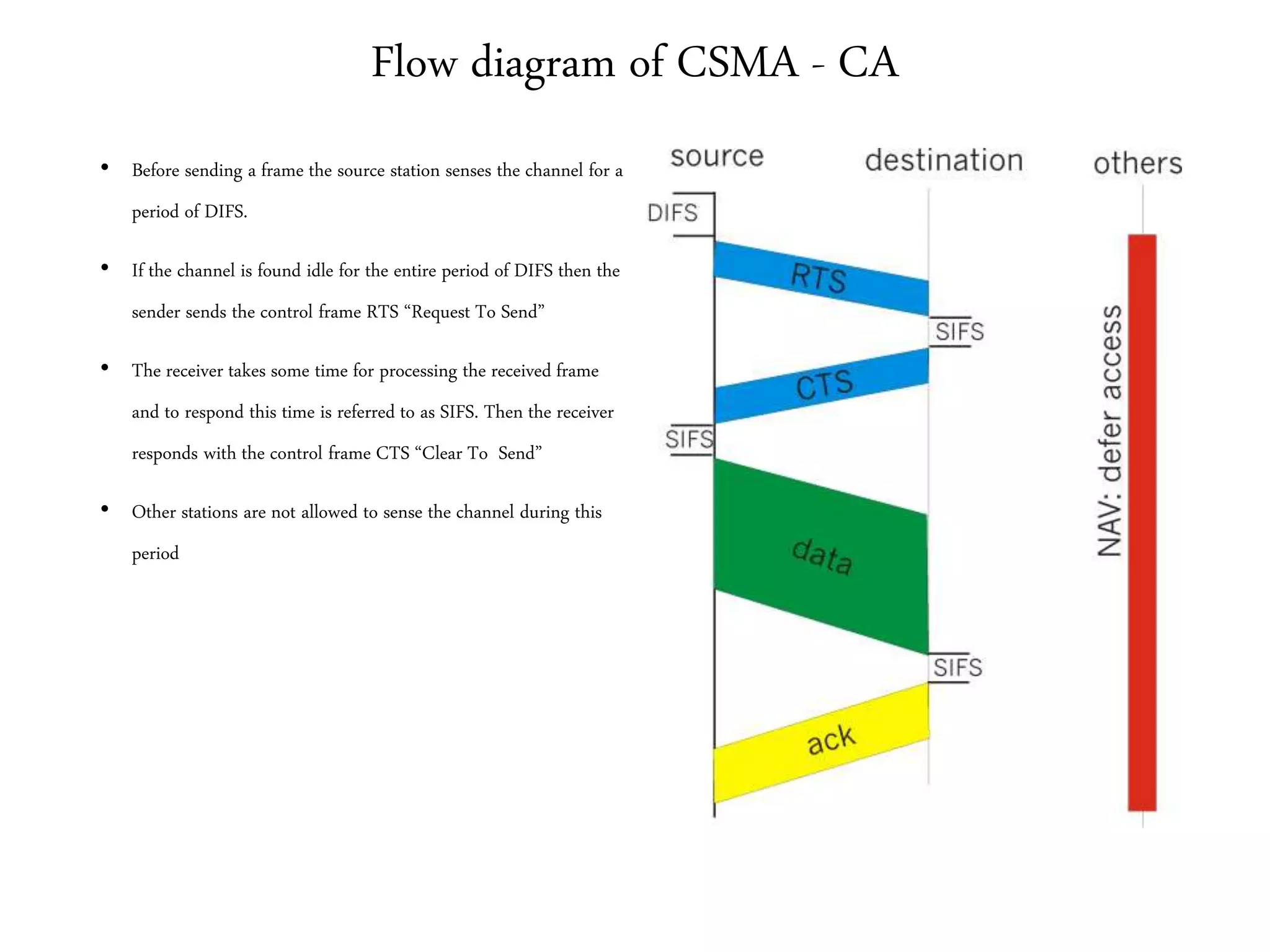
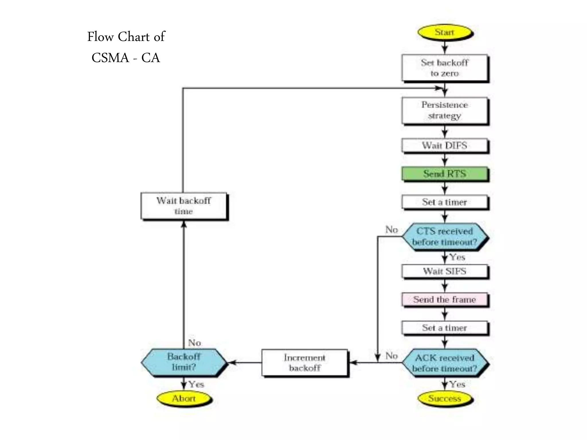
• Access Method – CSMA CA
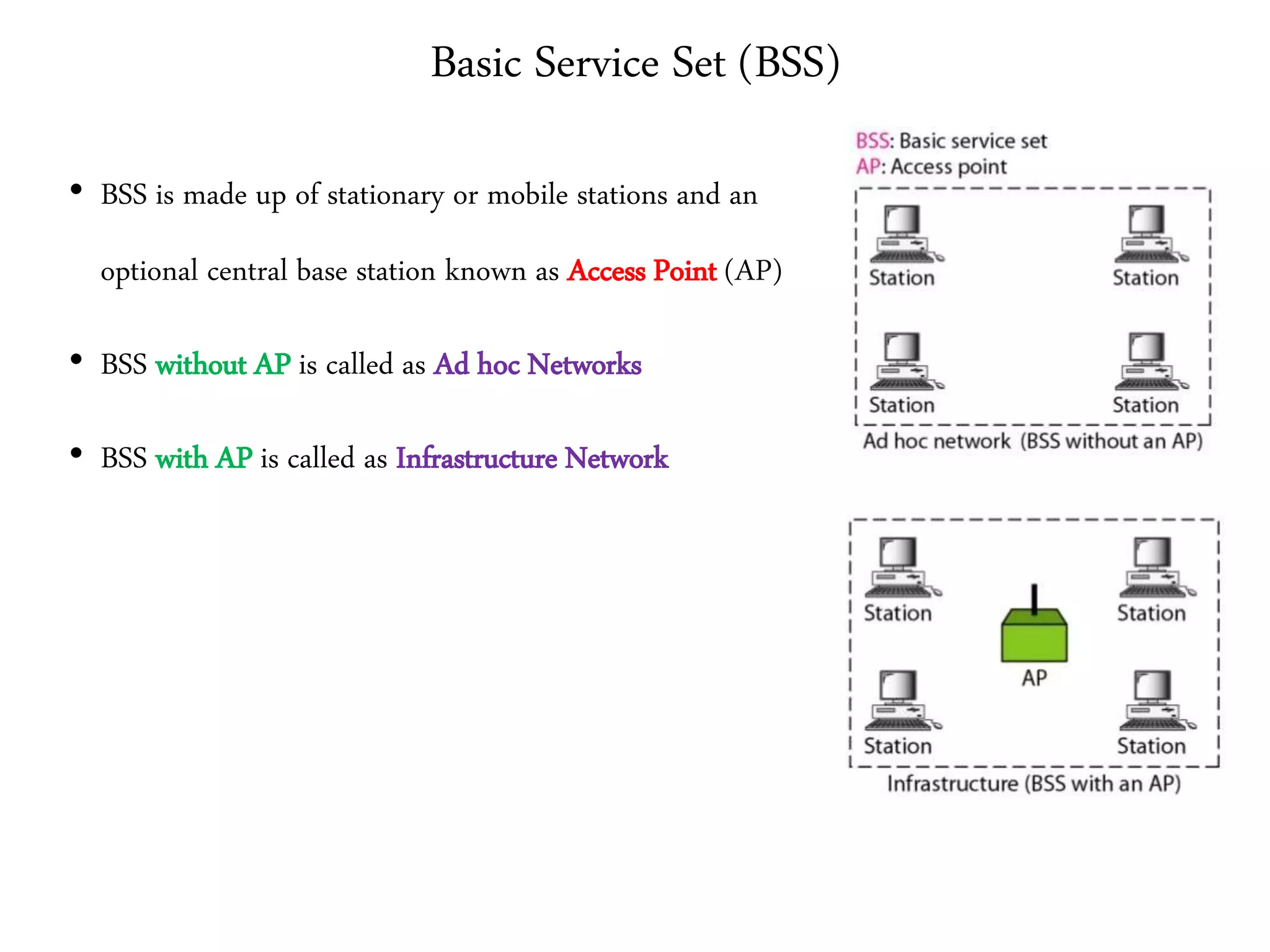
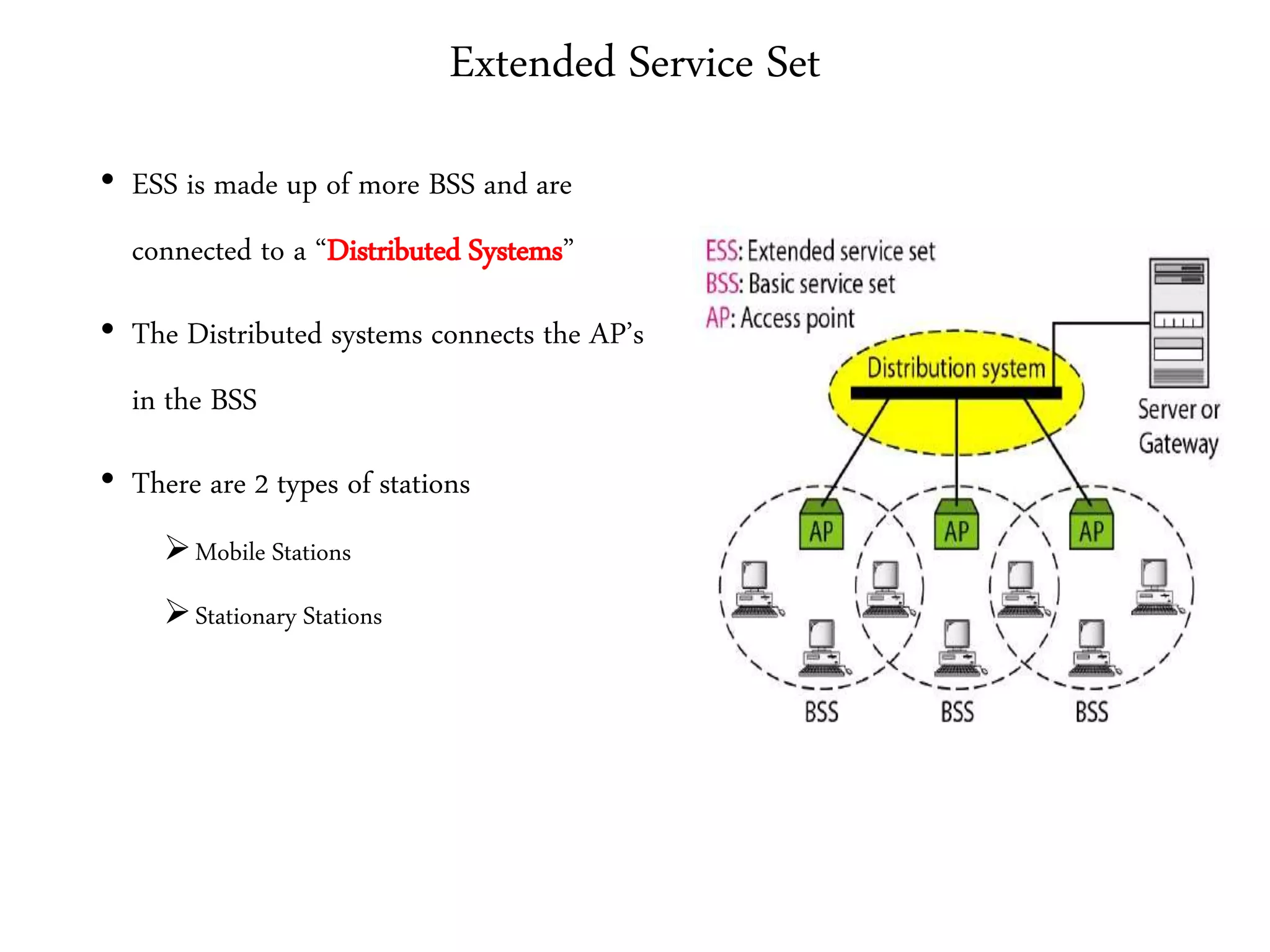
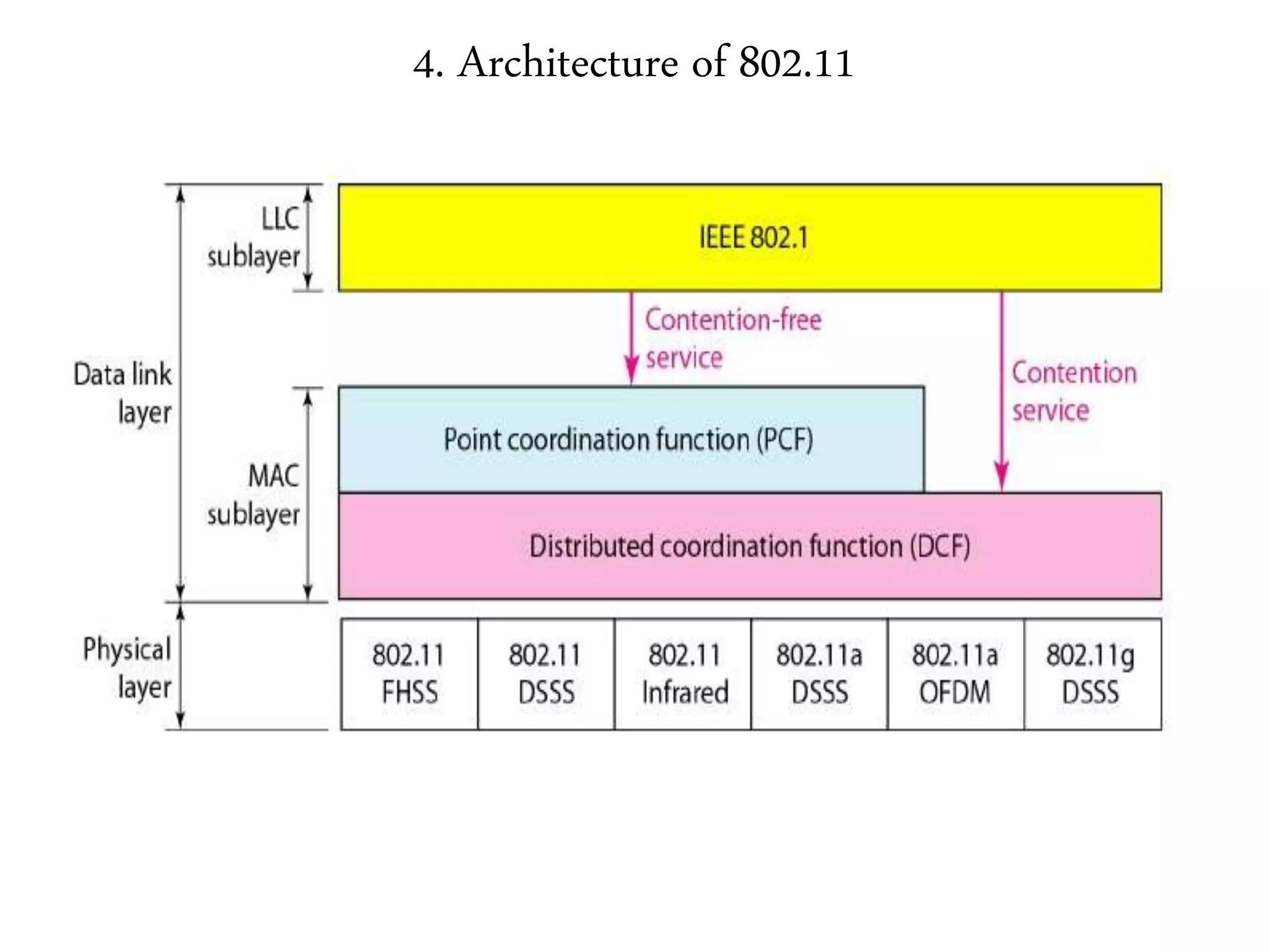
• Architecture
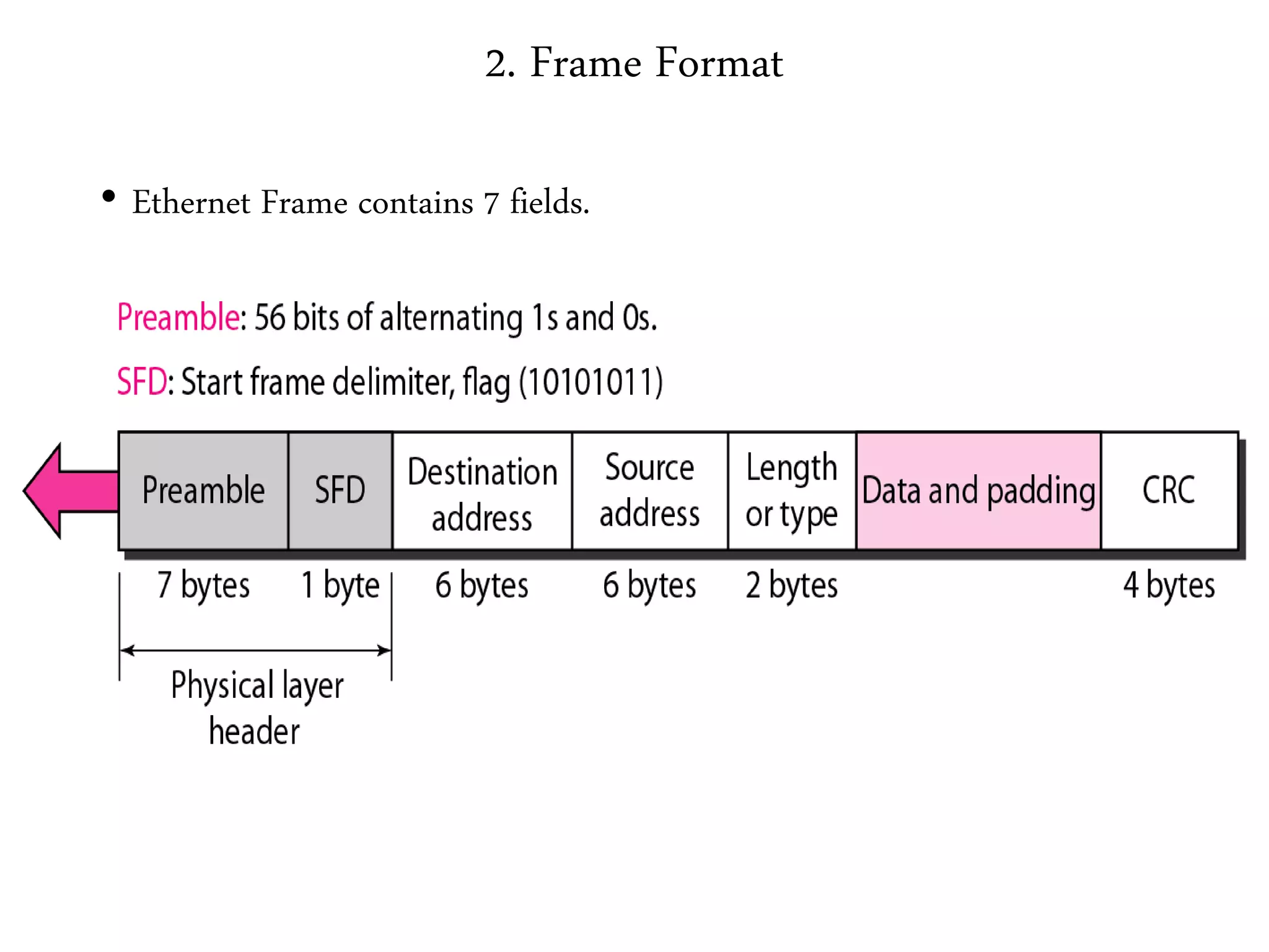
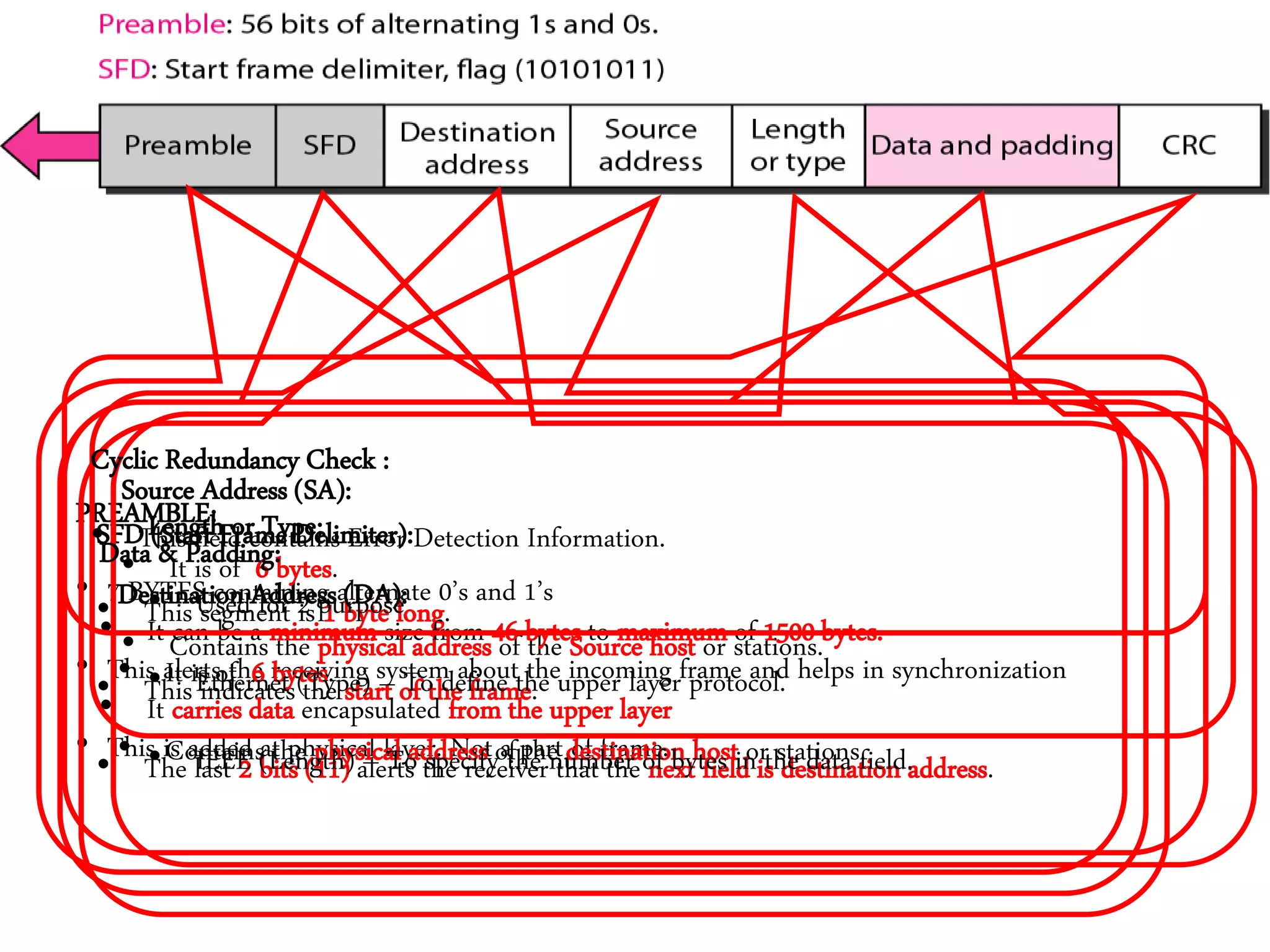
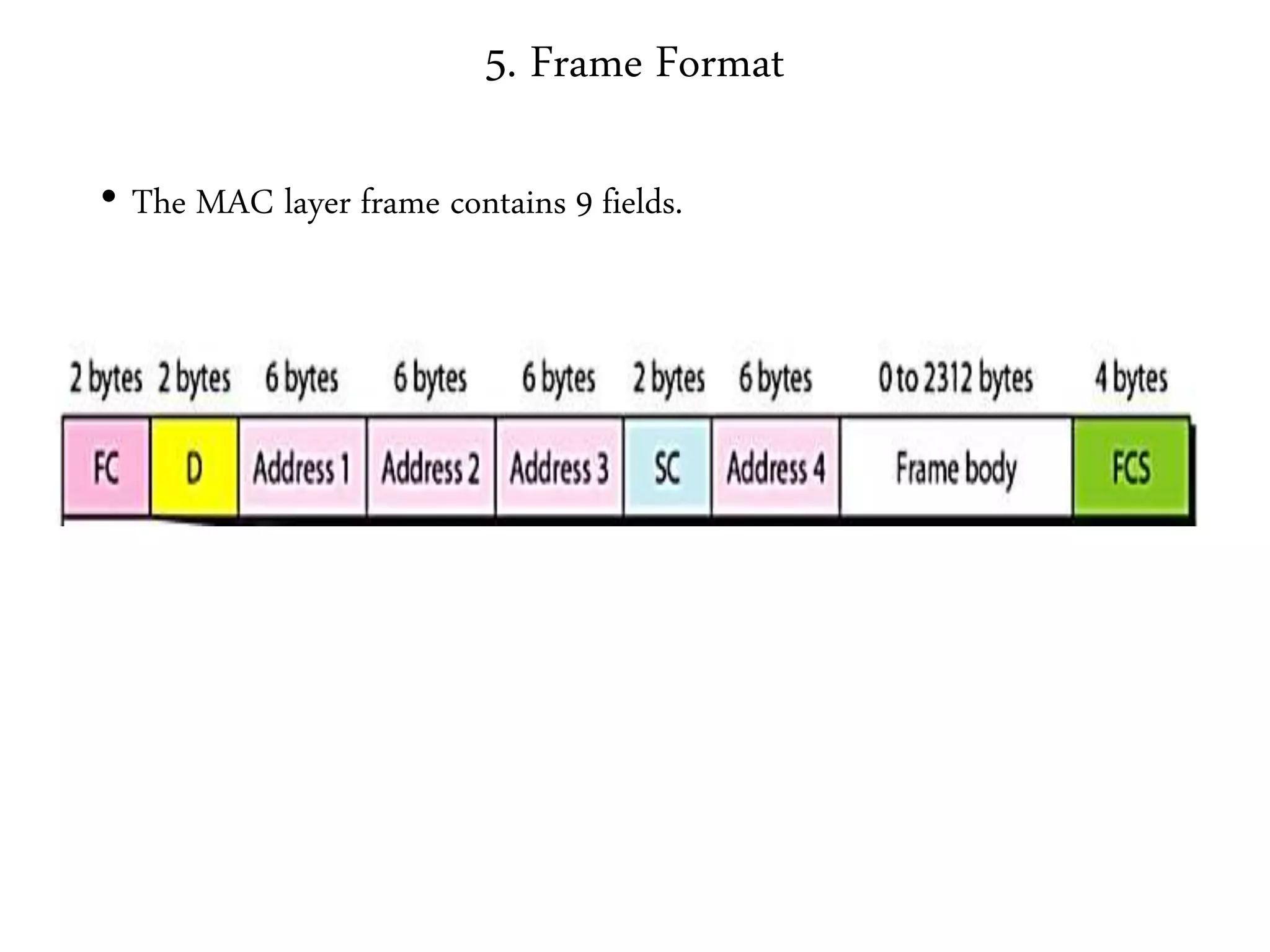
• Frame Format
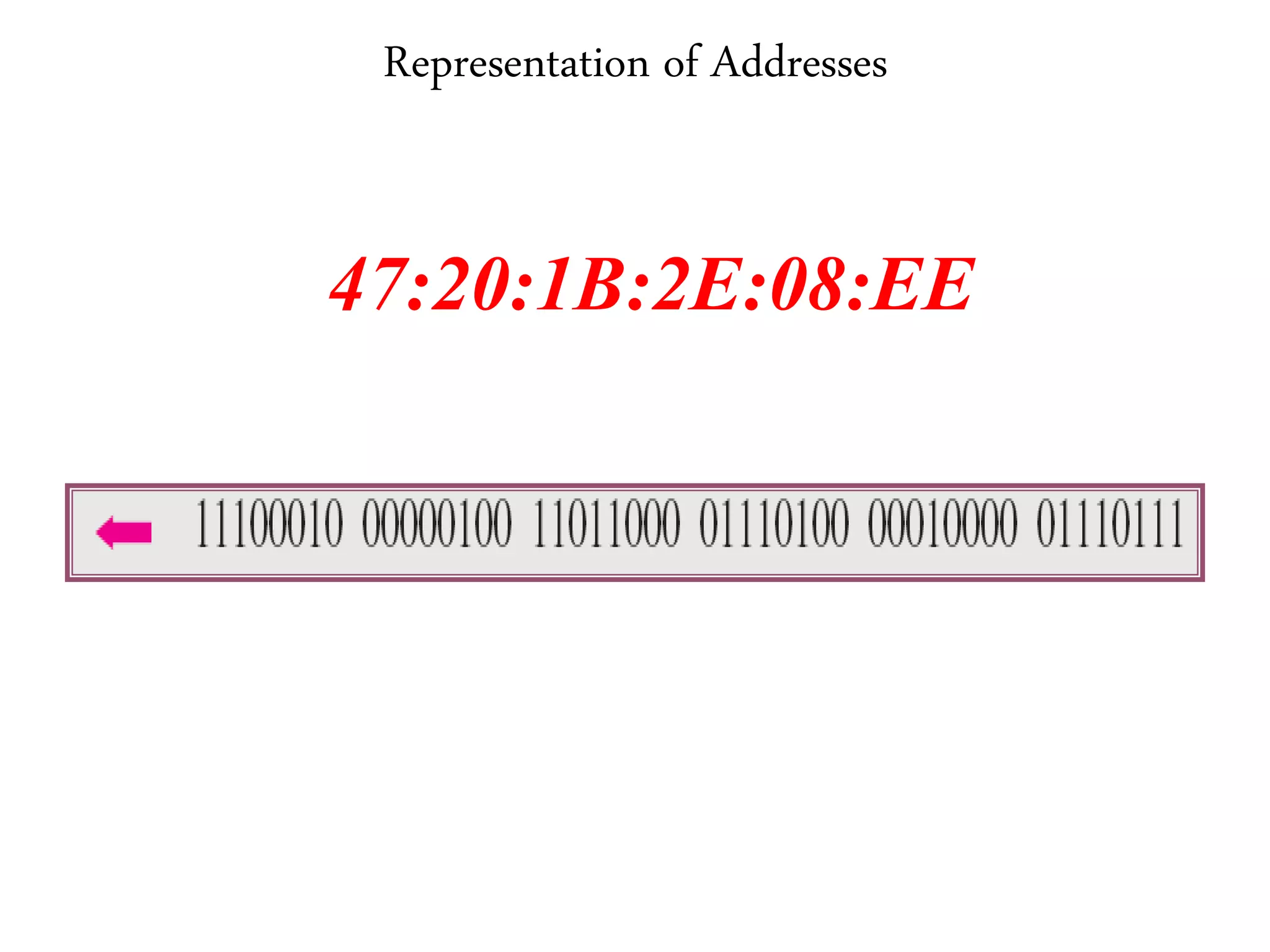
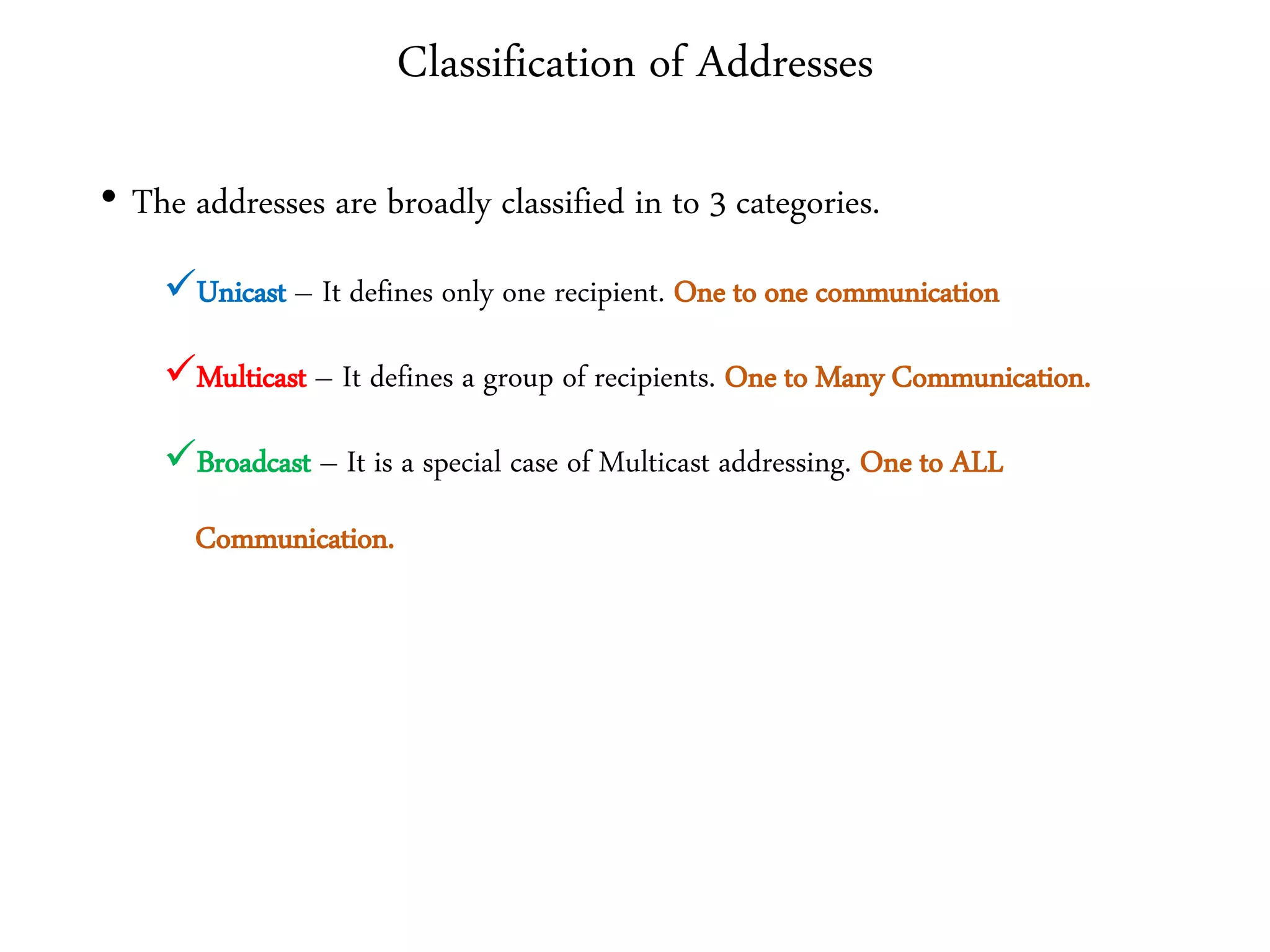
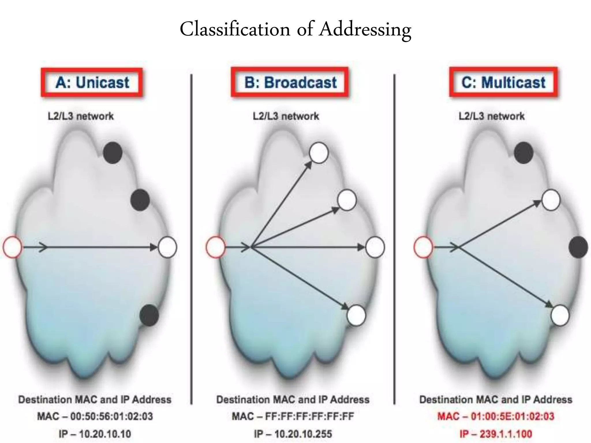
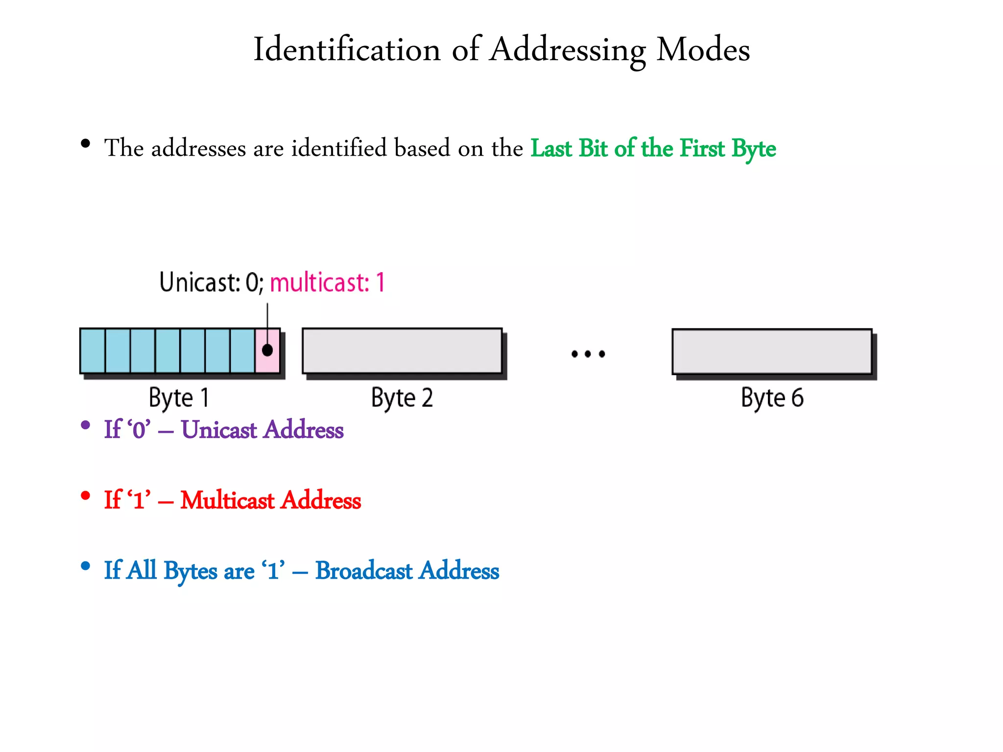
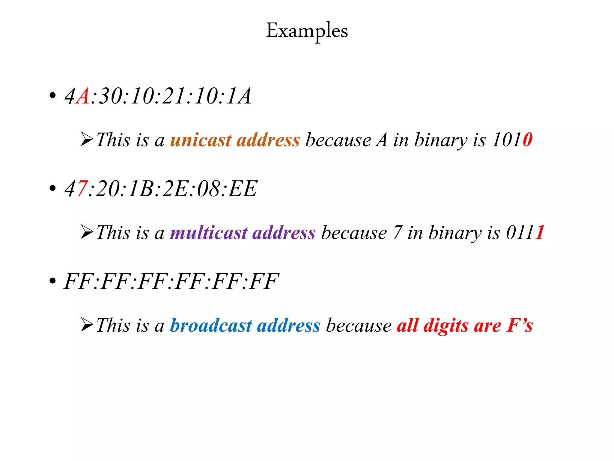
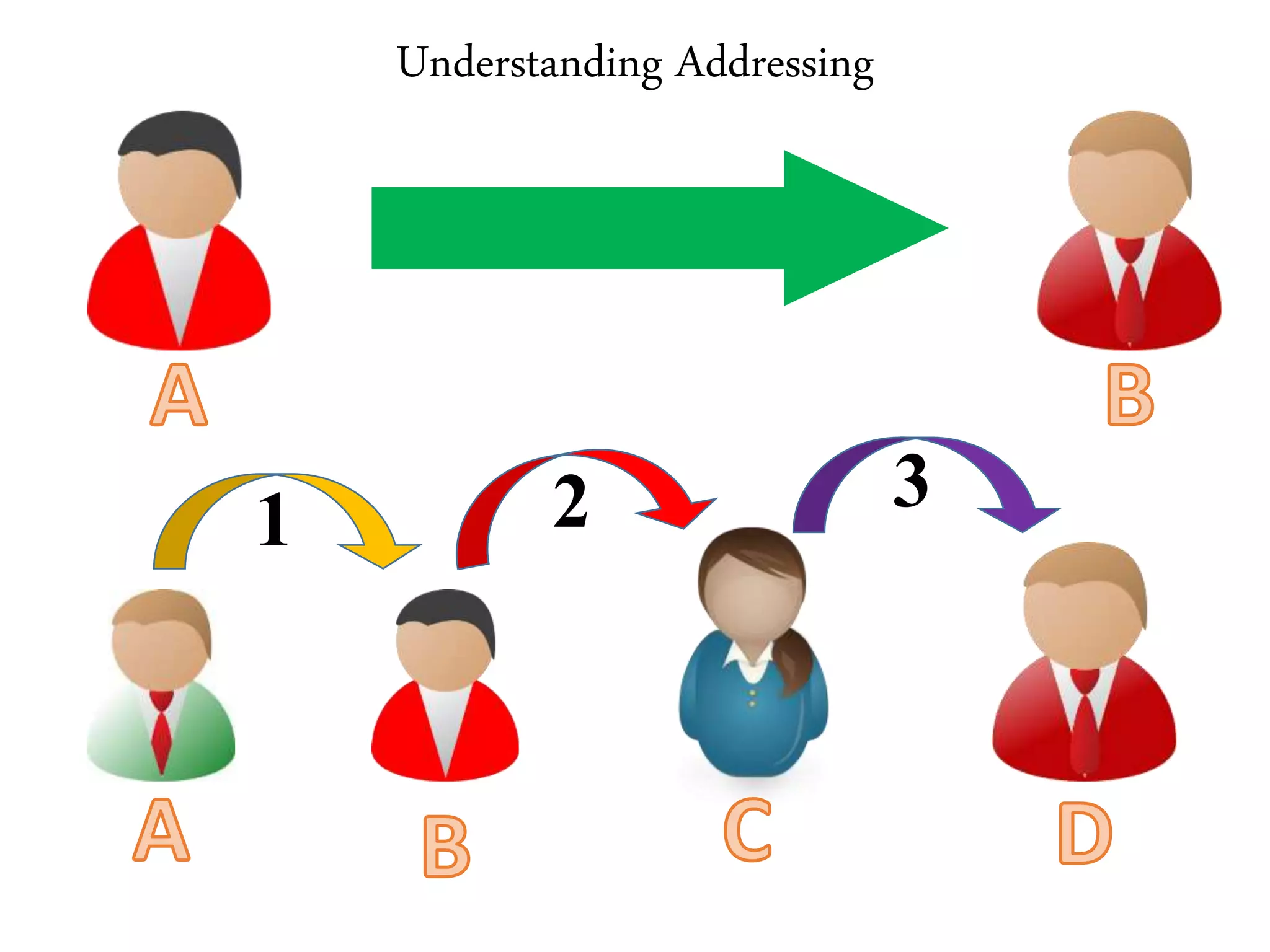
• Addressing Mechanisms](https://image.slidesharecdn.com/jg2wz2hsr2wsc6toimpi-signature-9bcd612675293d5941b62896d745c35646c89d8e395bf438351d48f0cd0d58ec-poli-170906151708/75/Computer-networks-unit-ii-45-2048.jpg)


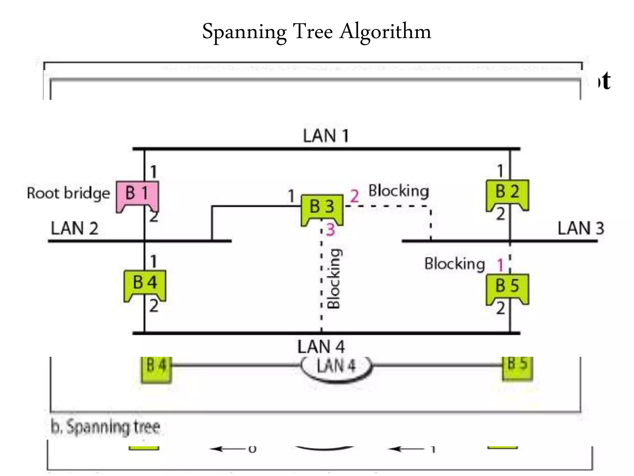
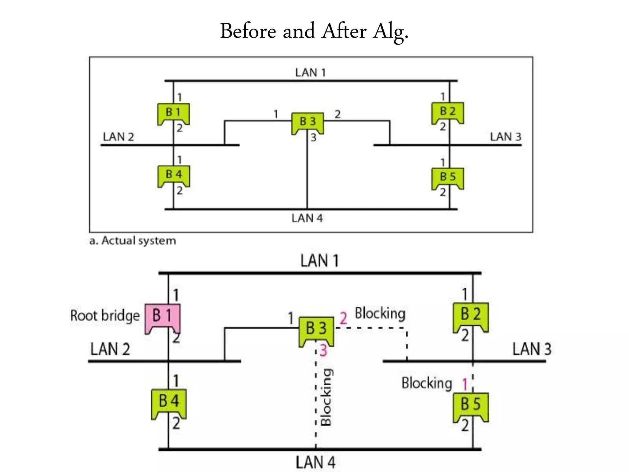

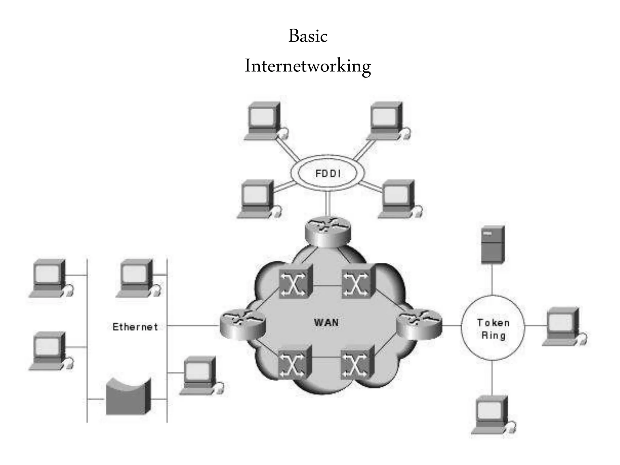


The document discusses computer networks and media access control. It covers topics like Ethernet, wireless LANs, Bluetooth, Wi-Fi, switching, bridging, IP, and more. The key points are: 1. It provides an overview of the topics to be discussed, including media access control, Ethernet standards, wireless technologies, and internetworking basics. 2. It summarizes the evolution of Ethernet and discusses its physical properties, frame format, addressing, and transmitter algorithm using CSMA/CD. 3. It describes wireless LAN standards like Bluetooth and Wi-Fi, addressing problems in wireless networks, and discussing concepts like spread spectrum, CSMA/CA, and network architectures.