Download as PDF, PPTX
![25
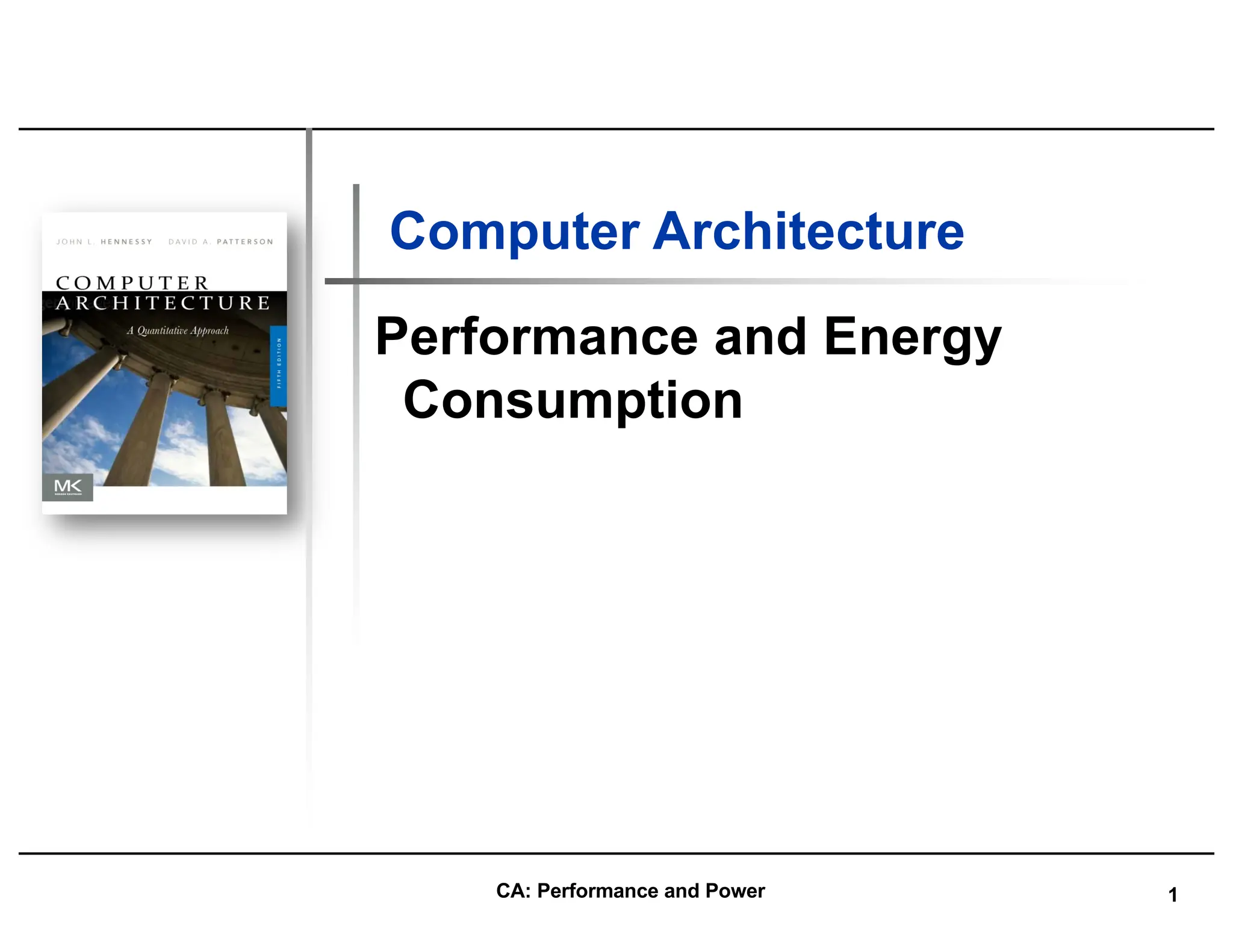
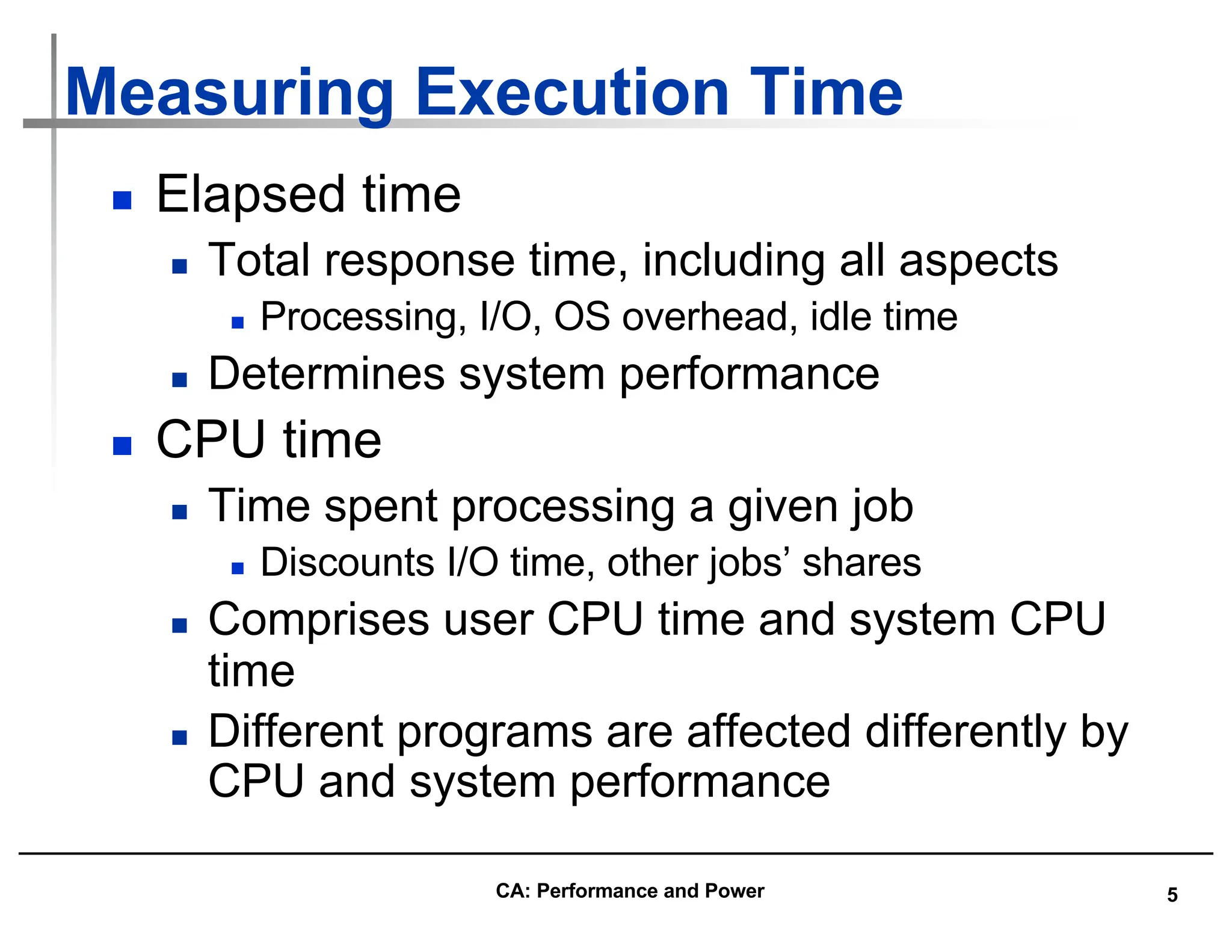
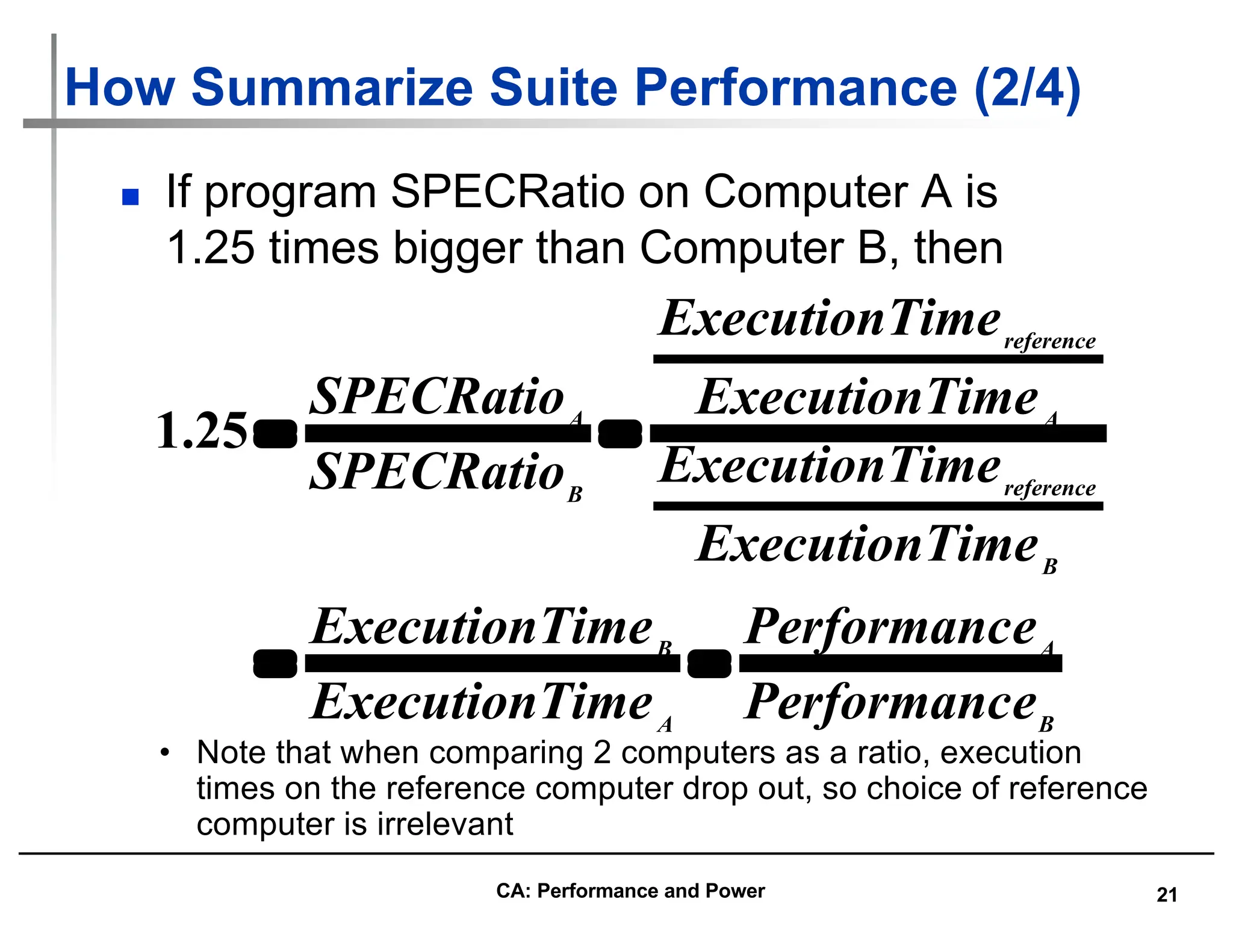
How Summarize Suite Performance (4/4)
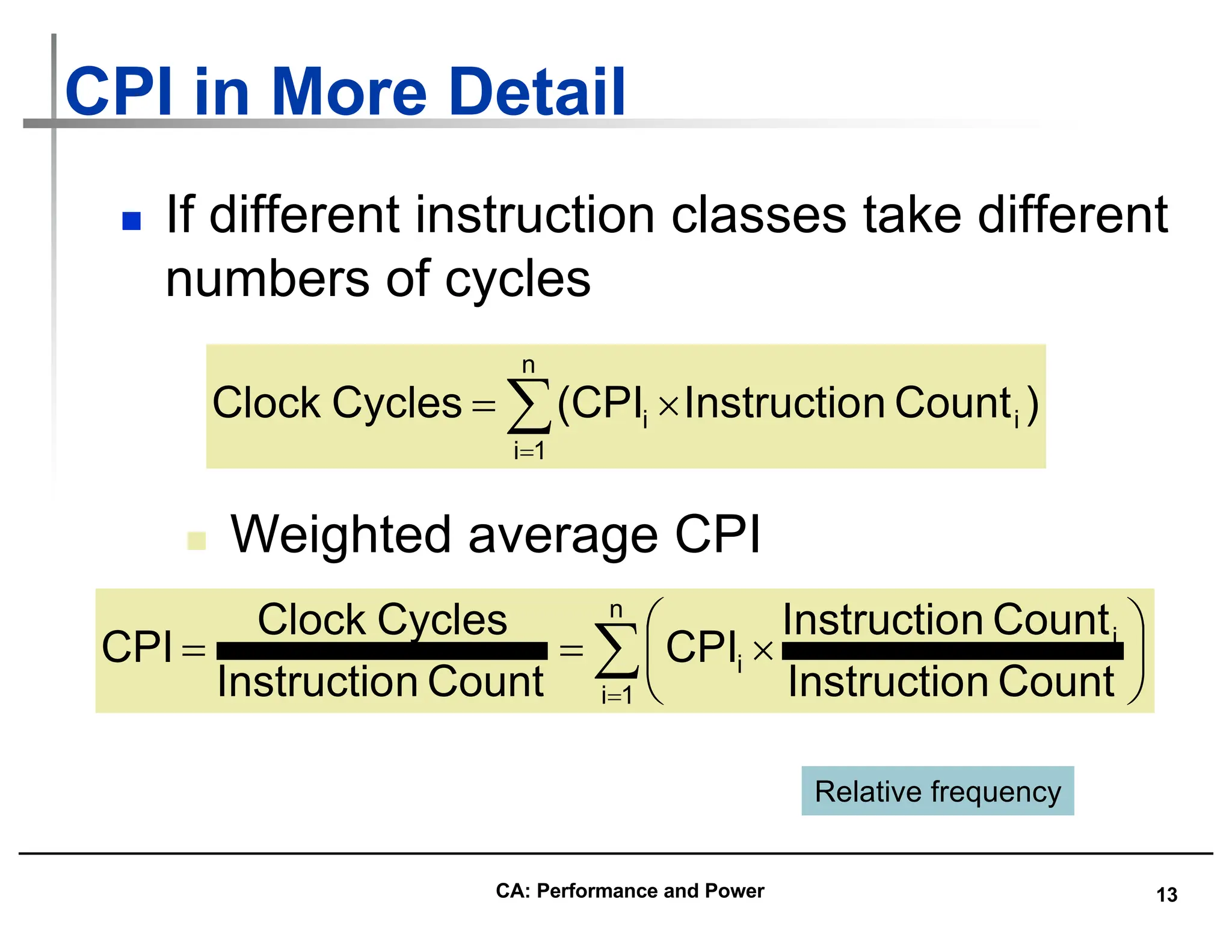
n Does a single mean well summarize performance of programs in
benchmark suite?
n Can decide if mean a good predictor by characterizing variability
of distribution using standard deviation
n Like geometric mean, geometric standard deviation is multiplicative
rather than arithmetic
n Can simply take the logarithm of SPECRatios, compute the standard
mean and standard deviation, and then take the exponent to convert
back:
n The geometric standard deviation, denoted by σg, is calculated as
follows: log σg=[1/n∑n
i=1(logxi−logG)2]1/2.
n where G=n√x1⋅x2⋅…⋅xn is the geometric mean of SPECRatios (x1 . xn).
( )
( )
( )
( )
i
n
i
i
SPECRatio
StDev
tDev
GeometricS
SPECRatio
n
ean
GeometricM
ln
exp
ln
1
exp
1
=
÷
ø
ö
ç
è
æ
´
= å
=
CA: Performance and Power](https://image.slidesharecdn.com/computerarchitectureperformanceandenergy-240127061813-86754b21/75/Computer-Architecture-Performance-and-Energy-25-2048.jpg)
![26
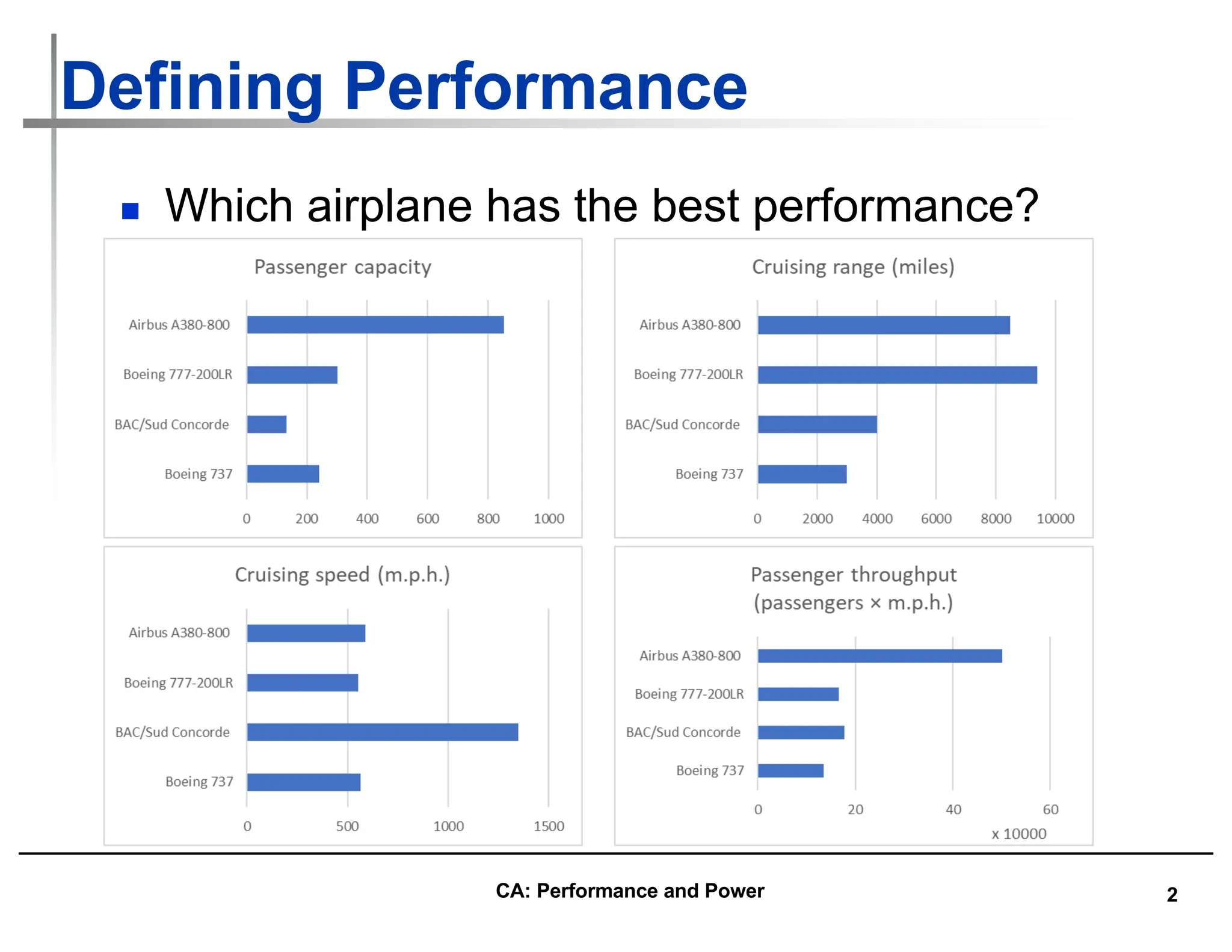
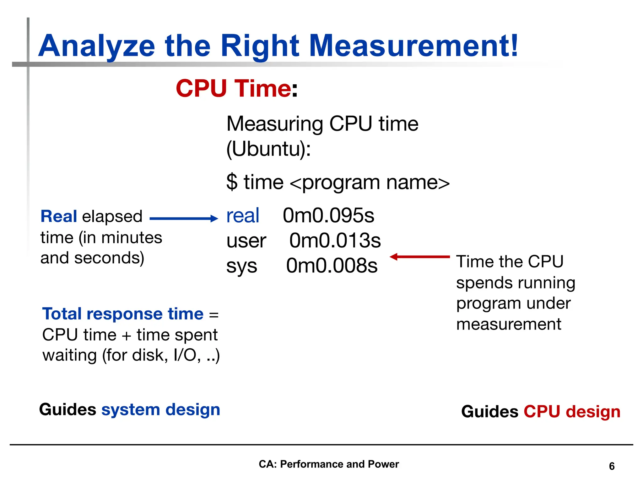
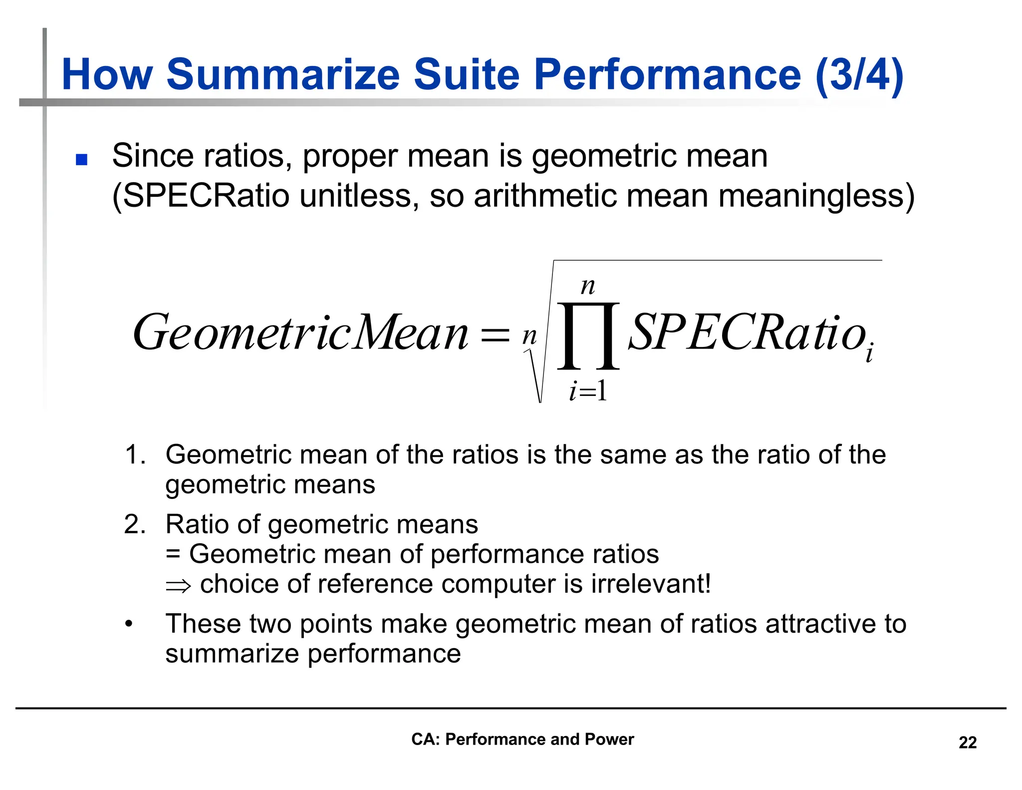
Example Standard Deviation: (1/3)
0
2000
4000
6000
8000
10000
12000
14000
wupwise
swim
mgrid
applu
mesa
galgel
art
equake
facerec
ammp
lucas
fma3d
sixtrack
apsi
SPECfpRatio
1372
5362
2712
GM = 2712
GStDev = 1.98
• GM and multiplicative StDev of SPECfp2000 for Itanium 2
Outside 1 StDev
Itanium 2 is
2712/100 times
as fast as Sun
Ultra 5 (GM), &
range within 1
Std. Deviation is
[13.72, 53.62]
CA: Performance and Power](https://image.slidesharecdn.com/computerarchitectureperformanceandenergy-240127061813-86754b21/75/Computer-Architecture-Performance-and-Energy-26-2048.jpg)
![27
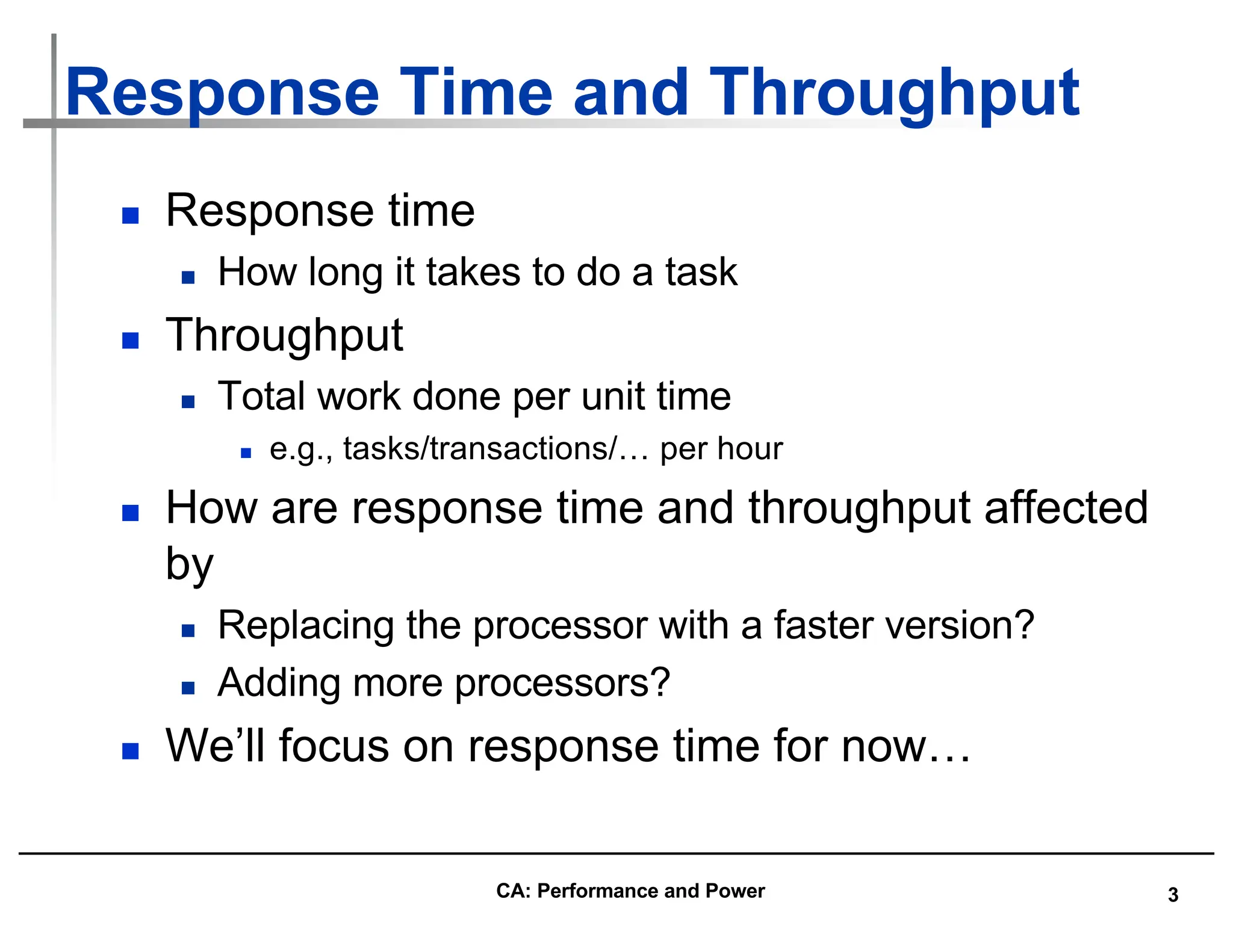
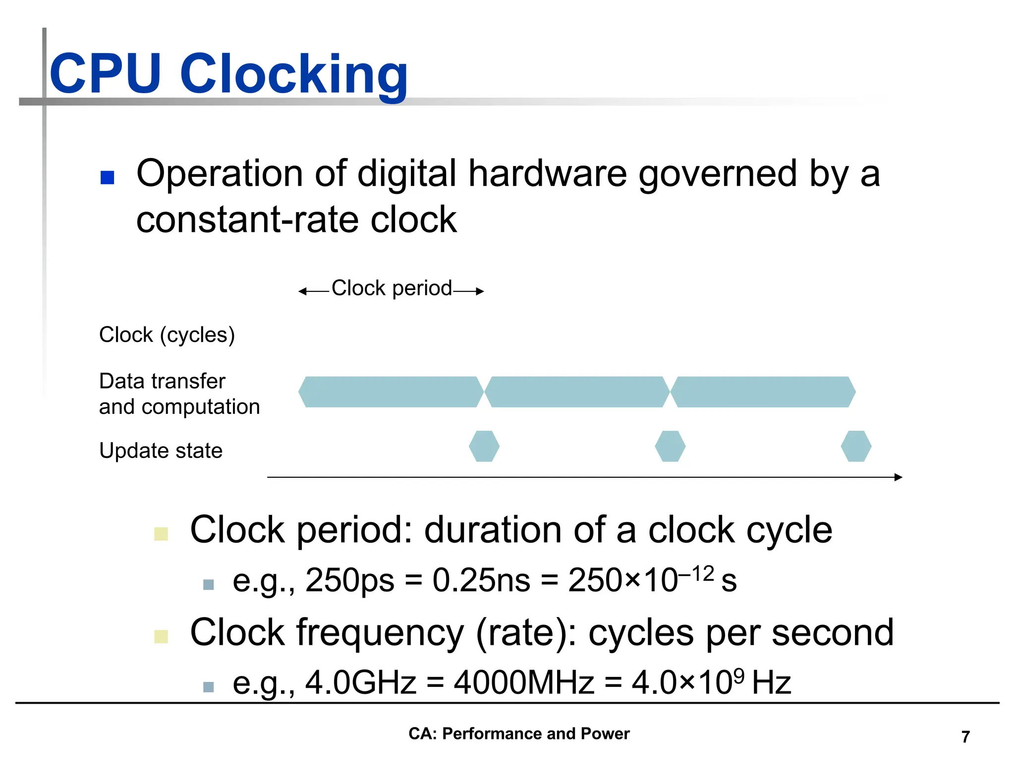
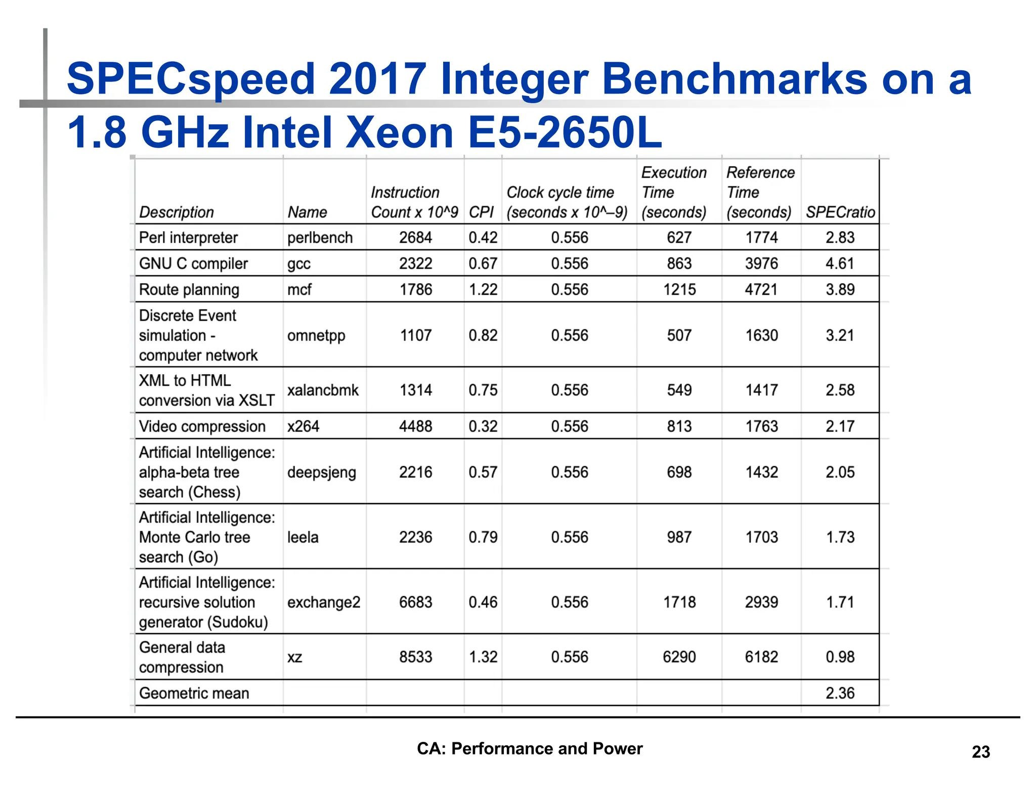
Example Standard Deviation : (2/3)
• GM and multiplicative StDev of SPECfp2000 for AMD Athlon
0
2000
4000
6000
8000
10000
12000
14000
wupwise
swim
mgrid
applu
mesa
galgel
art
equake
facerec
ammp
lucas
fma3d
sixtrack
apsi
SPECfpRatio
1494
2911
2086
GM = 2086
GStDev = 1.40
Outside 1 StDev
Athon is
2086/100 times
as fast as Sun
Ultra 5 (GM), &
range within 1
Std. Deviation is
[14.94, 29.11]
CA: Performance and Power](https://image.slidesharecdn.com/computerarchitectureperformanceandenergy-240127061813-86754b21/75/Computer-Architecture-Performance-and-Energy-27-2048.jpg)
![28
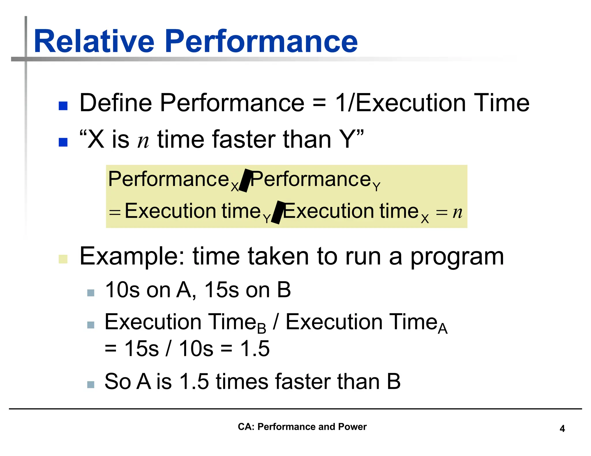
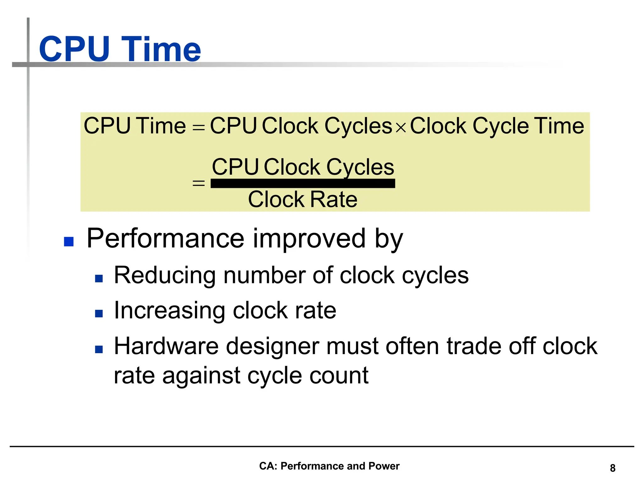
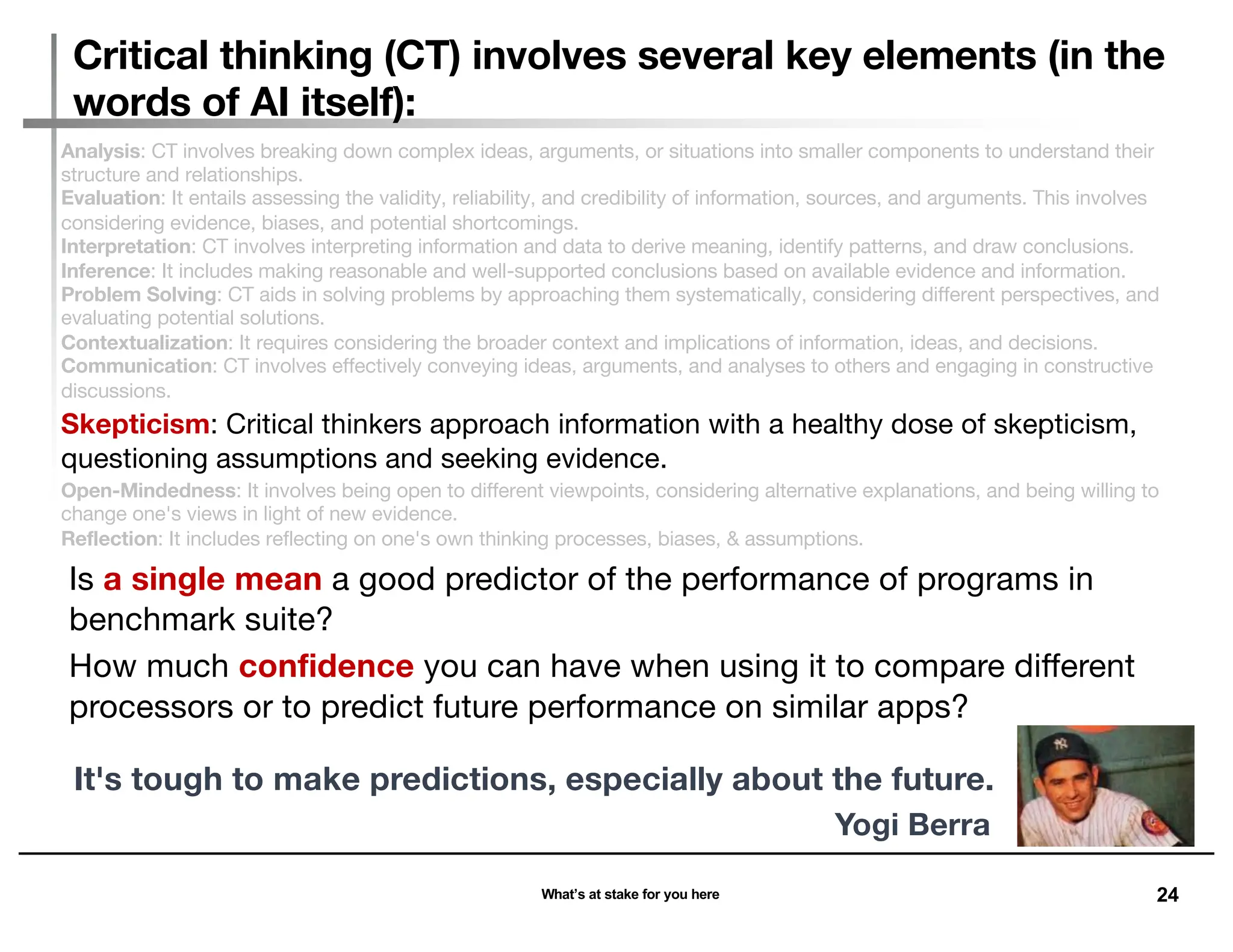
Example Standard Deviation (3/3)
-
0.50
1.00
1.50
2.00
2.50
3.00
3.50
4.00
4.50
5.00
wupwise
swim
mgrid
applu
mesa
galgel
art
equake
facerec
ammp
lucas
fma3d
sixtrack
apsi
Ratio
Itanium
2
v.
Athlon
for
SPECfp2000
0.75
2.27
1.30
GM = 1.30
GStDev = 1.74
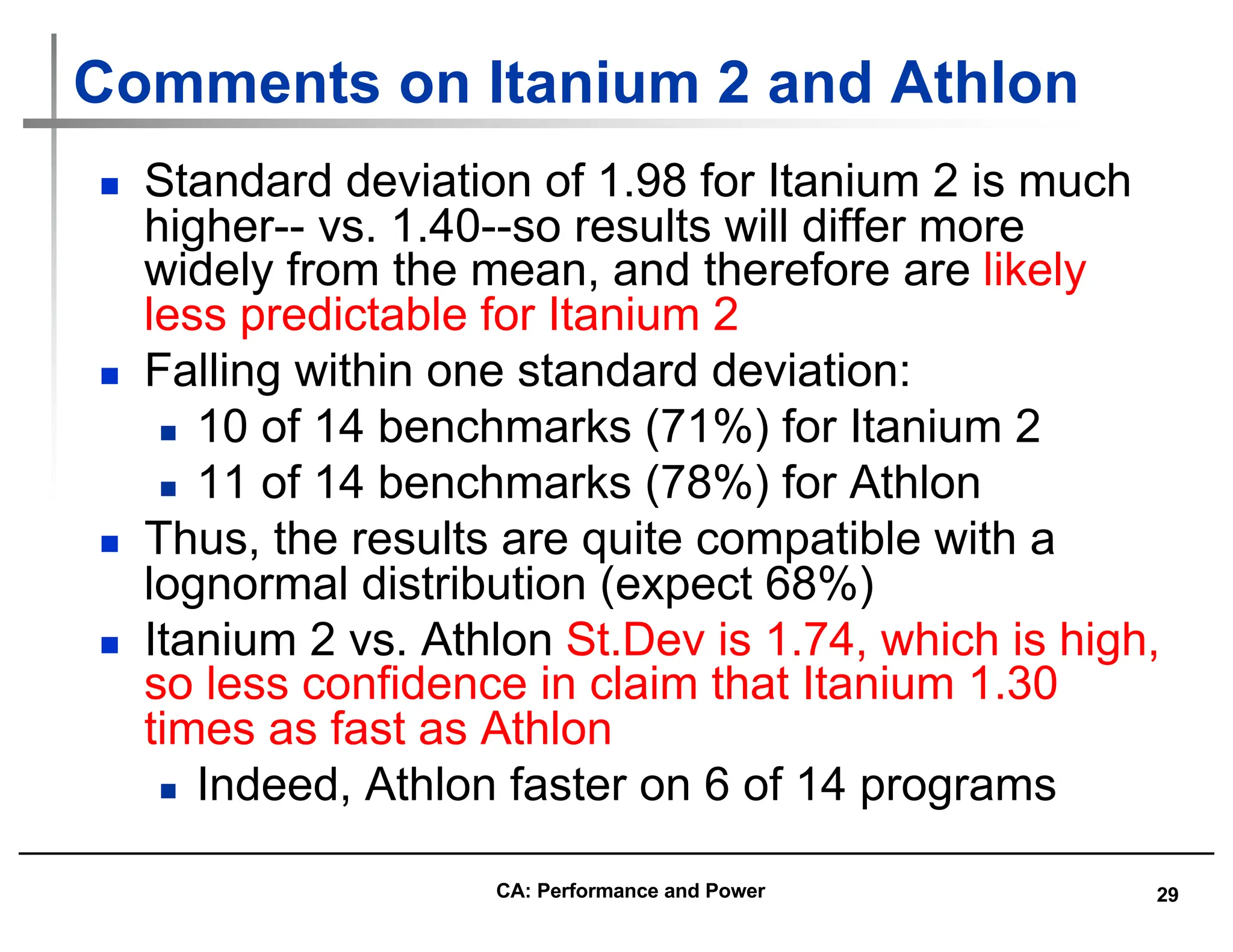
• GM and StDev Itanium 2 v Athlon
Outside 1 StDev
Ratio execution times (At/It) =
Ratio of SPECratios (It/At)
Itanium 2 1.30X Athlon (GM),
1 St.Dev. Range [0.75,2.27]
CA: Performance and Power](https://image.slidesharecdn.com/computerarchitectureperformanceandenergy-240127061813-86754b21/75/Computer-Architecture-Performance-and-Energy-28-2048.jpg)
![35
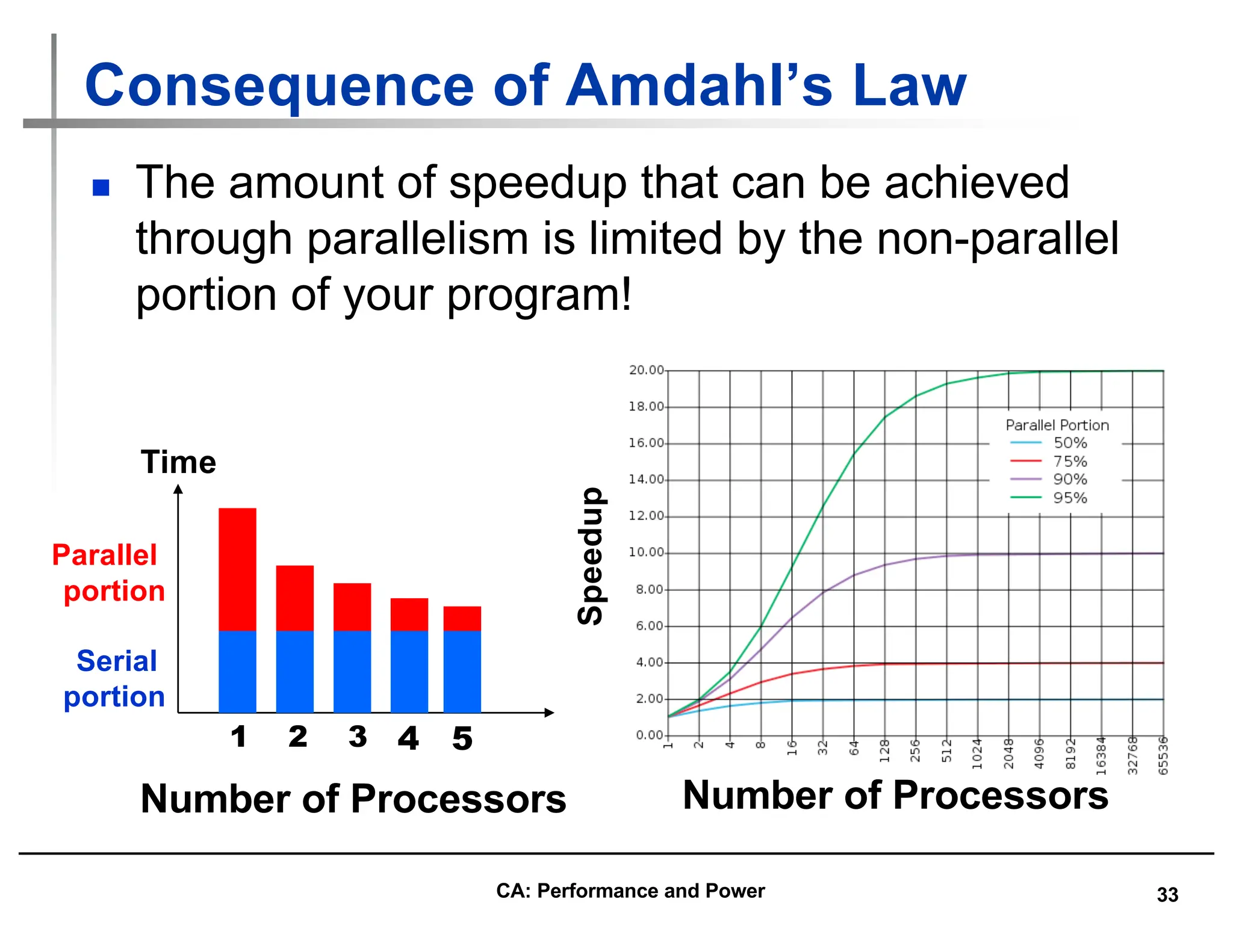
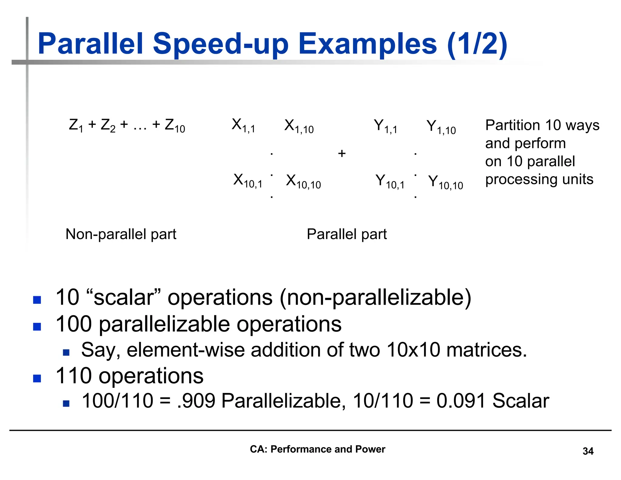
Parallel Speed-up Examples (2/2)
n Consider summing 10 scalar variables and two
10 by 10 matrices (matrix sum) on 10
processors
Speedup = 1/(.091 + .909/10) = 1/0.1819 = 5.5
n What if there are 100 processors ?
Speedup = 1/(.091 + .909/100) = 1/0.10009 = 10.0
n What if the matrices are 100 by 100 (or 10,010
adds in total) on 10 processors?
Speedup = 1/(.001 + .999/10) = 1/0.1009 = 9.9
n What if there are 100 processors ?
Speedup = 1/(.001 + .999/100) = 1/0.01099 = 91
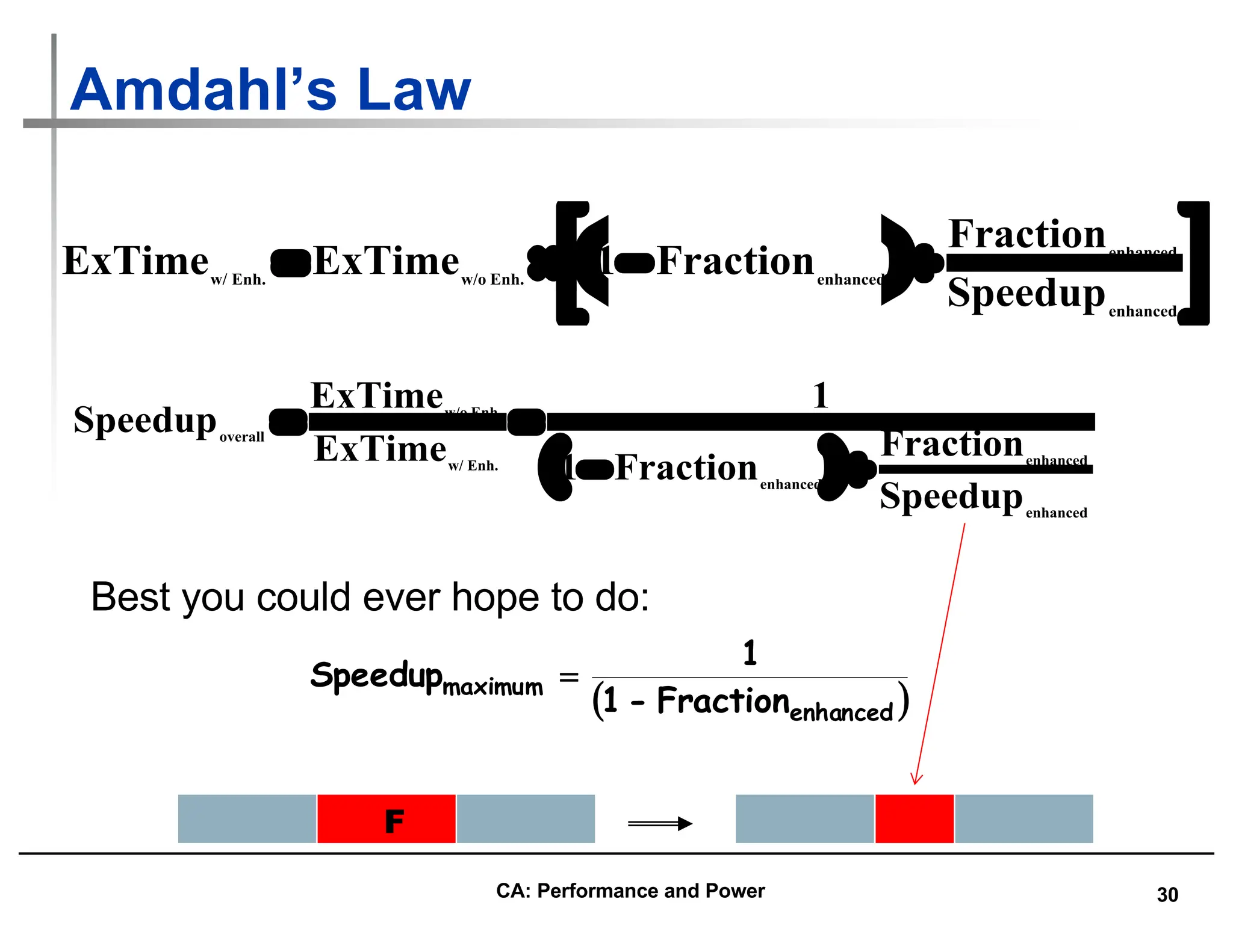
Speedup w/ E = 1 / [ (1-F) + F/S ]
CA: Performance and Power](https://image.slidesharecdn.com/computerarchitectureperformanceandenergy-240127061813-86754b21/75/Computer-Architecture-Performance-and-Energy-35-2048.jpg)
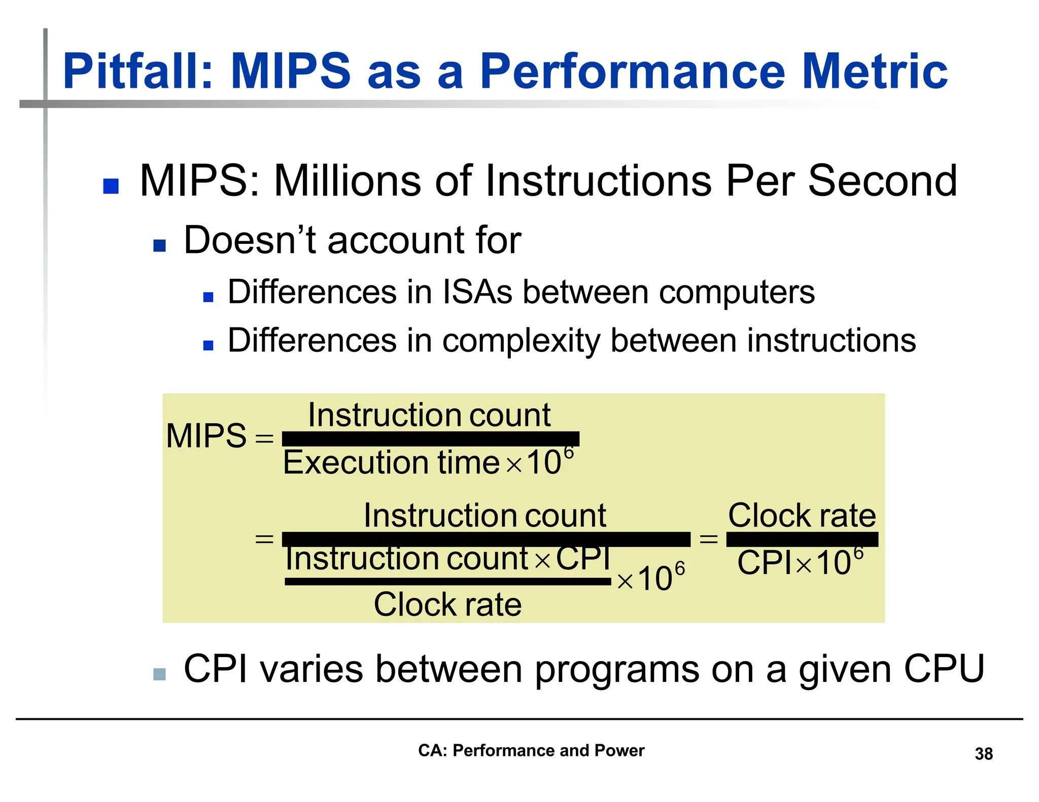

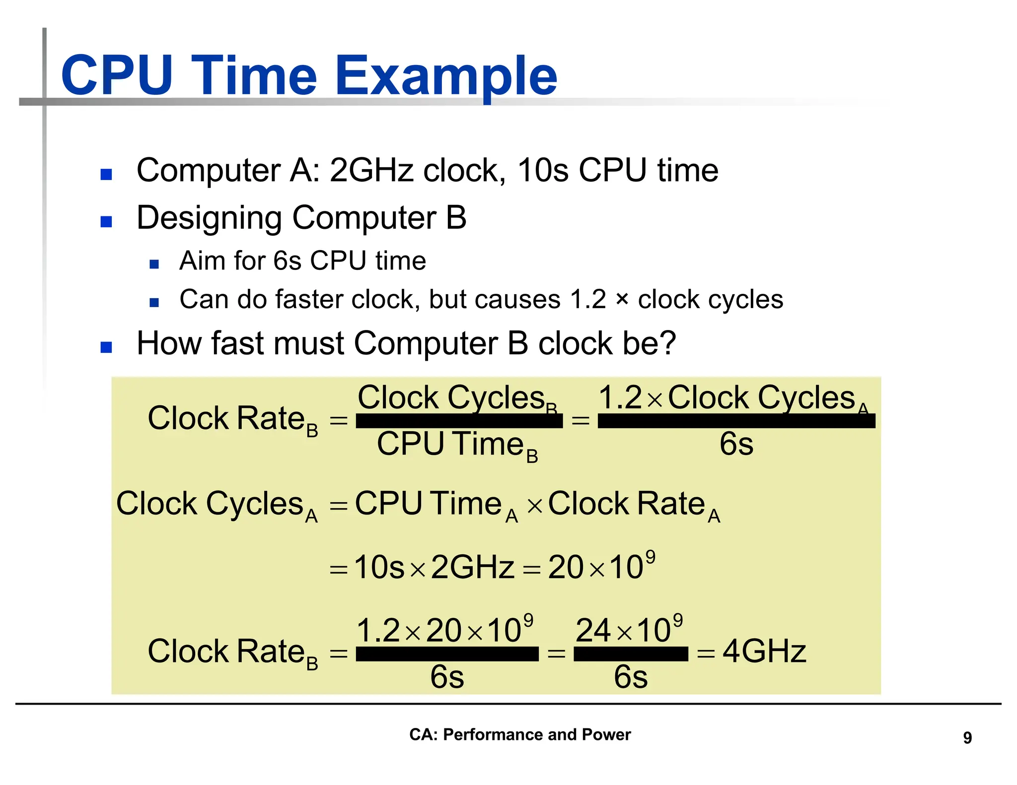
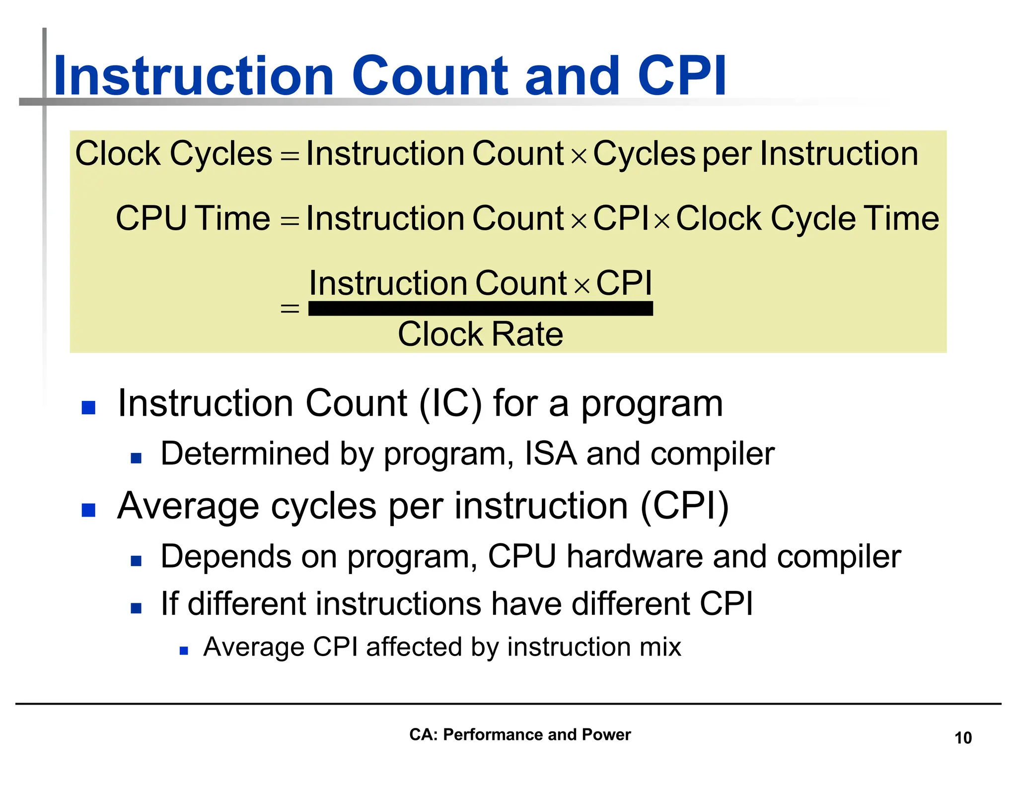
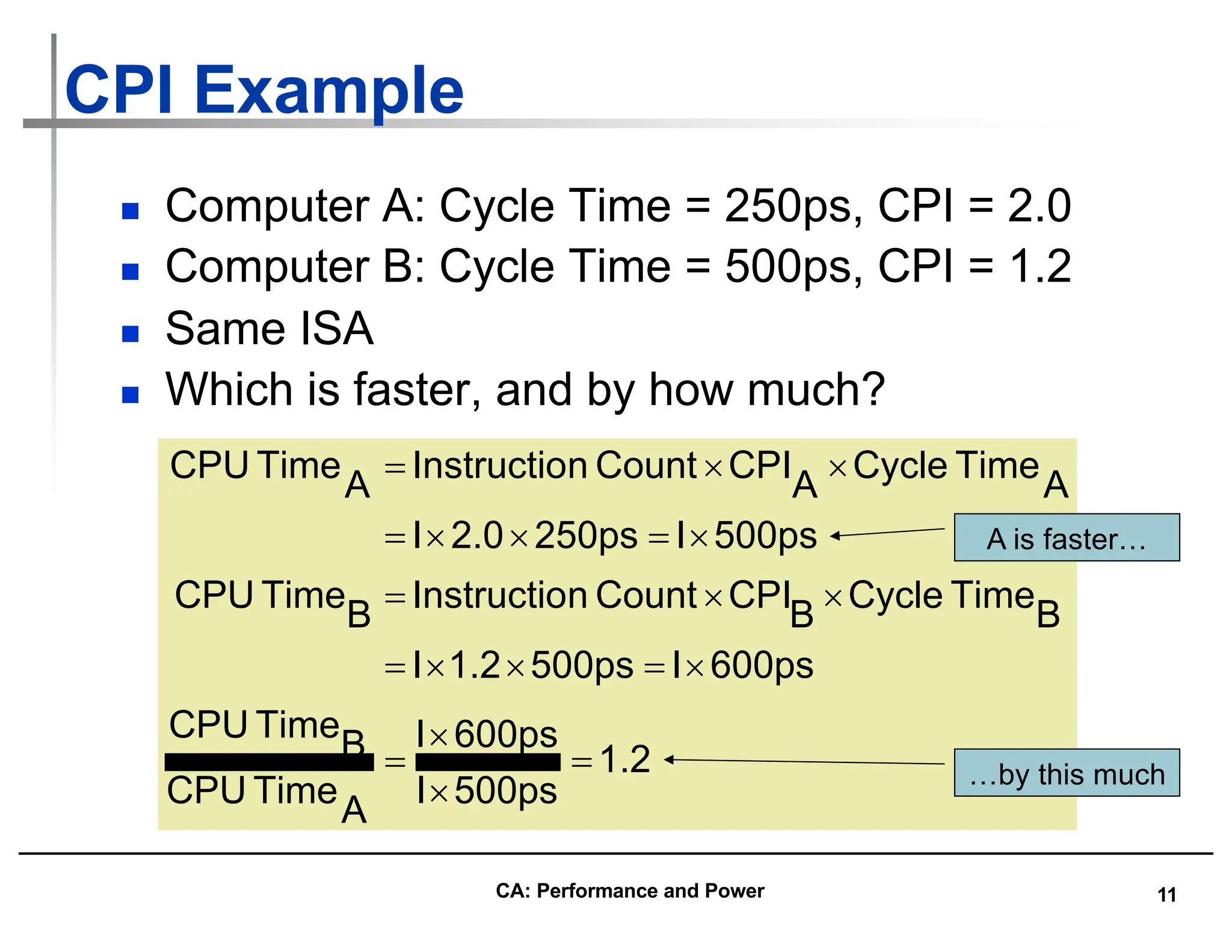
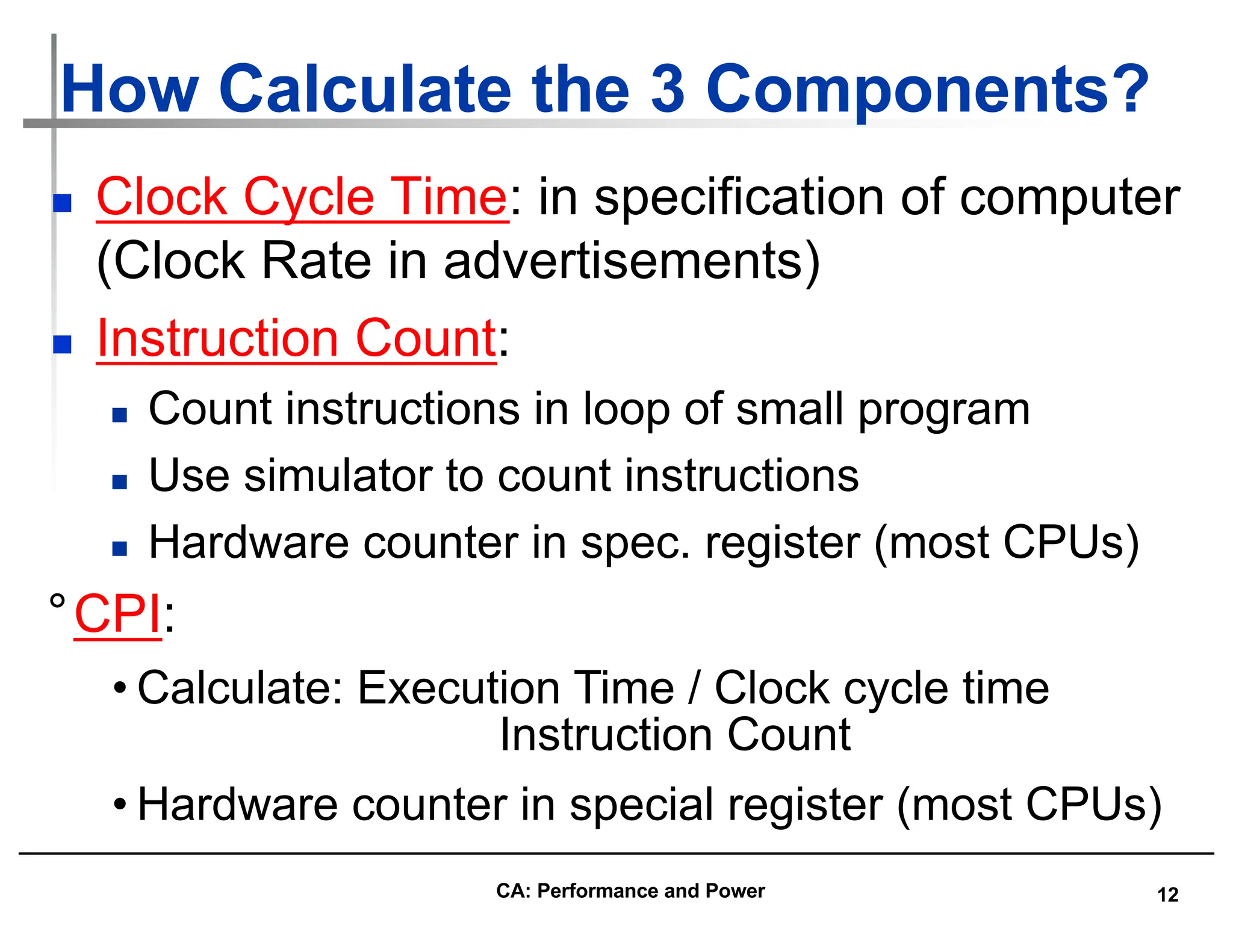
The document discusses computer architecture performance and energy consumption. It defines key performance metrics like response time and throughput. It also explains how to measure and calculate performance, including instruction count, clock cycles per instruction (CPI), and clock rate. The document emphasizes that performance depends on algorithms, programming languages, instruction sets, and technology. It discusses standardized benchmarks like SPEC CPU that are used to evaluate and compare overall processor performance using metrics like the geometric mean and geometric standard deviation of performance ratios.