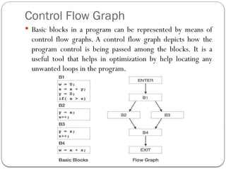
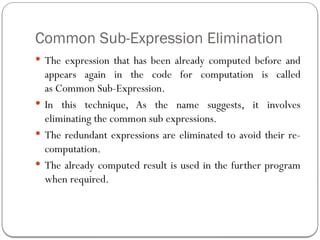
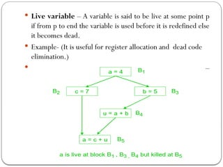
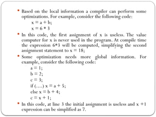
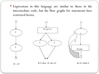
The document discusses code optimization techniques aimed at improving program performance by reducing resource consumption and enhancing execution speed. It covers types of optimization, such as machine-independent and machine-dependent optimization, along with various techniques like constant folding, common sub-expression elimination, and loop optimization. The importance of basic blocks and data flow analysis in the optimization process is also highlighted, demonstrating how these methods can lead to more efficient code.

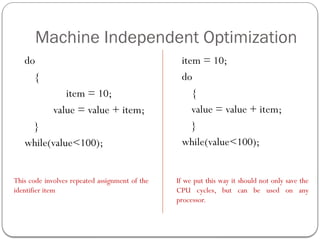
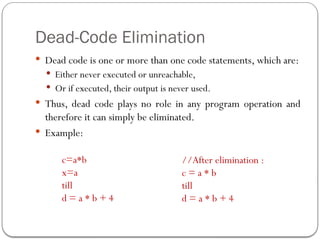
![Example
Code Before Optimization Code After Optimization
S1 = 4 * i
S2 = a[S1]
S3 = 4 * j
S4 = 4 * i //Redundant Expression
S5 = n
S6 = b[S4] + S5
S1 = 4 * i
S2 = a[S1]
S3 = 4 * j
S5 = n
S6 = b[S1] + S5](https://image.slidesharecdn.com/unit-51585393640-250127070235-eaa8d171/85/complier-design-unit-5-for-helping-students-14-320.jpg)
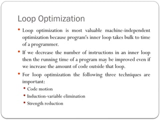
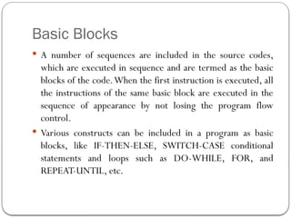
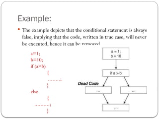
![Reduction in Strength
Strength reduction is used to replace the expensive operation
by the cheaper once on the target machine.
Addition of a constant is cheaper than a multiplication. So we
can replace multiplication with an addition within the loop.
Multiplication is cheaper than exponentiation. So we can
replace exponentiation with multiplication within the loop.
while (i<10)
{
j= 3 * i+1;
a[j]=a[j]-2;
i=i+2;
}
s= 3*i+1;
while (i<10)
{
j=s;
a[j]= a[j]-2;
i=i+2;
s=s+6;
}
After strength reduction](https://image.slidesharecdn.com/unit-51585393640-250127070235-eaa8d171/85/complier-design-unit-5-for-helping-students-18-320.jpg)
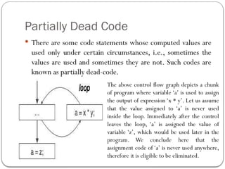
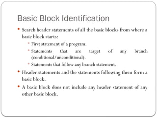
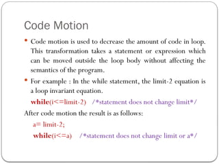
![Partial Redundancy
Redundant expressions are computed more than once in
parallel path, without any change in operands. whereas
partial-redundant expressions are computed more than once
in a path, without any change in operands.
[redundant expression] [partially redundant expression]](https://image.slidesharecdn.com/unit-51585393640-250127070235-eaa8d171/85/complier-design-unit-5-for-helping-students-22-320.jpg)
![ We define a portion of a flow graph called a region to be a
set of nodes N that includes a header, which dominates all
other nodes in the region. All edges between nodes in
N are in the region, except for some that enter the header.
We say that the beginning points of the dummy blocks at
the entry and exit of a statement’s region are the
beginning and end points, respectively, of the statement.
The equations are inductive, or syntax-directed,
definition of the sets in[S], out[S], gen[S], and kill[S]
for all statements S.
gen[S] is the set of definitions “generated” by S while kill[S]
is the set of definitions that never reach the end of S.
Consider the following data-flow equations for reaching
definitions :](https://image.slidesharecdn.com/unit-51585393640-250127070235-eaa8d171/85/complier-design-unit-5-for-helping-students-37-320.jpg)
![d
gen [S] = { d }
kill [S] = Da – { d }
out [S] = gen [S] U ( in[S] – kill[S] )
Observe the rules for a single assignment of variable a. Surely
that assignment is a definition of a, say d.Thus
Gen[S]={d}
On the other hand, d “kil s” all other definitions of a, so we write
Kill[S] = Da – {d}
Where, Da is the set of all definitions in the program for variable a.](https://image.slidesharecdn.com/unit-51585393640-250127070235-eaa8d171/85/complier-design-unit-5-for-helping-students-38-320.jpg)
![ Under what circumstances is definition d generated by S=S1; S2?
First of all, if it is generated by S2, then it is surely generated by
S. if d is generated by S1, it will reach the end of S provided it is
not killed by S2.Thus, we write
gen[S]=gen[S2] U (gen[S1]-kill[S2])
Similar reasoning applies to the killing of a definition, so we have
Kill[S] = kill[S2] U (kill[S1] – gen[S2])
gen[S]=gen[S2] U (gen[S1]-kill[S2])
Kill[S] = kill[S2] U (kill[S1] – gen[S2])
in [S1] = in [S] in [S2] = out [S1]
out [S] = out [S2]](https://image.slidesharecdn.com/unit-51585393640-250127070235-eaa8d171/85/complier-design-unit-5-for-helping-students-39-320.jpg)