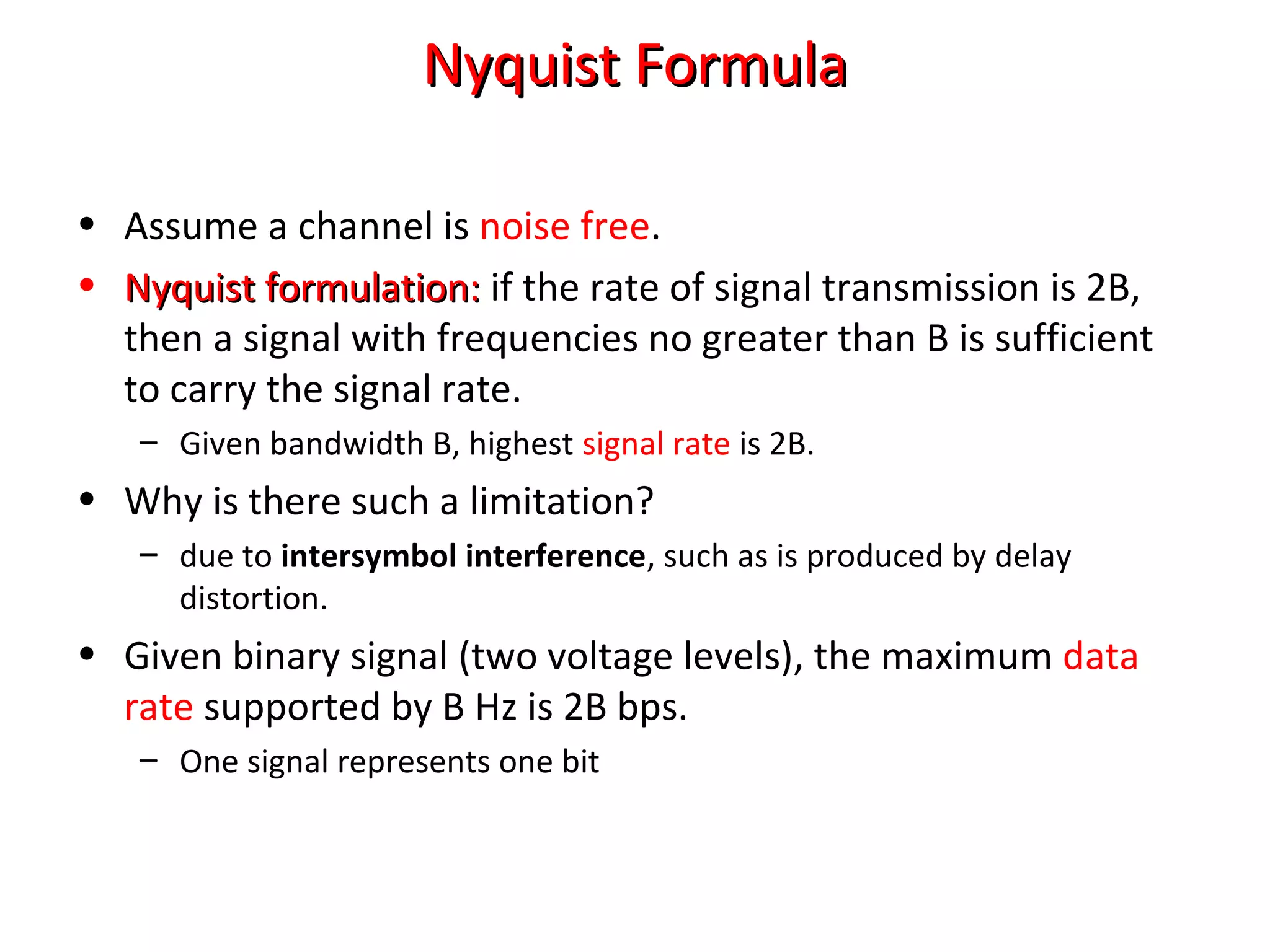
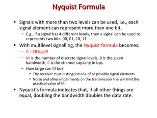
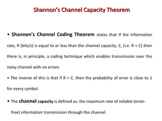
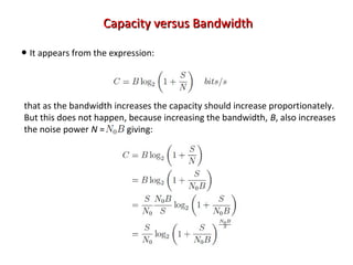
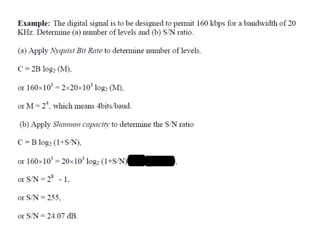
The Nyquist formula states that the maximum data rate supported by a bandwidth B is 2B bits per second. Doubling the bandwidth doubles the maximum data rate. Signals with more than two levels can represent more data per signal, with the formula becoming C = 2B log2M, where M is the number of signal levels. Shannon's channel capacity theorem defines the maximum reliable transmission rate C for a bandwidth B channel as C = B log2(1 + S/N), where S is the signal power and N is the noise power.

1. NyquistNyquist FormulaFormula
• Assume a channel is noise free.
• Nyquist formulation:Nyquist formulation: if the rate of signal transmission is 2B,
then a signal with frequencies no greater than B is sufficient
to carry the signal rate.
– Given bandwidth B, highest signal rate is 2B.
• Why is there such a limitation?
– due to intersymbol interference, such as is produced by delay
distortion.
• Given binary signal (two voltage levels), the maximum data
rate supported by B Hz is 2B bps.
– One signal represents one bit

2. NyquistNyquist FormulaFormula
• Signals with more than two levels can be used, i.e., each
signal element can represent more than one bit.
– E.g., if a signal has 4 different levels, then a signal can be used to
represents two bits: 00, 01, 10, 11
• With multilevel signalling, the Nyquist formula becomes:
– C = 2B log2M
– M is the number of discrete signal levels, B is the given
bandwidth, C is the channel capacity in bps.
– How large can M be?
• The receiver must distinguish one of M possible signal elements.
• Noise and other impairments on the transmission line will limit the
practical value of M.
• Nyquist’s formula indicates that, if all other things are
equal, doubling the bandwidth doubles the data rate.

3. Channel CapacityChannel Capacity
• Channel capacity is concerned with the information handling capacity of a
given channel. It is affected by:
– The attenuation of a channel which varies with frequency as well as
channel length.
– The noise induced into the channel which increases with distance.
– Non-linear effects such as clipping on the signal.
Some of the effects may change with time e.g. the frequency response of a
copper cable changes with temperature and age.

4. Obviously we need a way to model a channel in order to estimate how much
information can be passed through it. Although we can compensate for non
linear effects and attenuation it is extremely difficult to remove noise.
The highest rate of information that can be transmitted through a
channel is called the channel capacity, C.
Channel CapacityChannel Capacity

5. • Shannon’s Channel Coding Theorem states that if the information
rate, R (bits/s) is equal to or less than the channel capacity, C, (i.e. R < C) then
there is, in principle, a coding technique which enables transmission over the
noisy channel with no errors.
• The inverse of this is that if R > C, then the probability of error is close to 1
for every symbol.
• The channel capacity is defined as: the maximum rate of reliable (error-
free) information transmission through the channel.
Shannon’s Channel Capacity TheoremShannon’s Channel Capacity Theorem

6. Shannon’s Channel Capacity TheoremShannon’s Channel Capacity Theorem
• Shannon’s Channel Capacity Theorem (or the Shannon-Hartley
Theorem) states that:
where C is the channel capacity, B is the channel bandwidth in hertz, S is
the signal power and N is the noise power ( with being the
two sided noise PSD).
Note: S/N is the ratio watt/watt not dB.

7. • The channel capacity, C, increases as the available bandwidth increases and
as the signal to noise ratio increases (improves).
• This expression applies to information in any format and to both analogue
and data communications, but its application is most common in data
communications.
• The channel capacity theorem is one of the most important results of
information theory. In a single formula it highlights the interplay between 3
key system parameters:
– channel bandwidth,
– average transmitted or received signal power,
– noise power at the channel output.
Shannon’s Channel Capacity TheoremShannon’s Channel Capacity Theorem

8. • For a given average transmitted power S and channel bandwidth, B, we
can
transmit information at the rate C bits/s with no error, by employing
sufficiently complex coding systems. It is not possible to transmit at a rate
higher than C bits/s by any coding system without a definite probability of
error. Hence the channel capacity theorem defines the fundamental limit
on the rate of error-free transmission for a power-limited, band-limited
channel.
Shannon’s Channel Capacity TheoremShannon’s Channel Capacity Theorem

9. Capacity versus BandwidthCapacity versus Bandwidth
• It appears from the expression:
that as the bandwidth increases the capacity should increase proportionately.
But this does not happen, because increasing the bandwidth, B, also increases
the noise power N = giving:

10. Capacity versus BandwidthCapacity versus Bandwidth

12. Transmission ImpairmentsTransmission Impairments
• With any communications system, the signal that is received
may differ from the signal that is transmitted, due to various
transmission impairments.
• Consequences:
– For analog signals: degradation of signal quality
– For digital signals: bit errors
• The most significant impairments include
– Attenuation and attenuation distortion
– Delay distortion
– Noise

14. AttenuationAttenuation
• Attenuation: signal strength falls off with distance.
• Depends on medium
– For guided media, the attenuation is generally exponential and thus
is typically expressed as a constant number of decibels per unit
distance.
– For unguided media, attenuation is a more complex function of
distance and the makeup of the atmosphere.
• Three considerations for the transmission engineer:
1. A received signal must have sufficient strength so that the
electronic circuitry in the receiver can detect the signal.
2. The signal must maintain a level sufficiently higher than noise to be
received without error.
These two problems are dealt with by the use of amplifiers
or repeaters.

15. Attenuation DistortionAttenuation Distortion
(Following the previous slide)
Attenuation is often an increasing function of frequency. This
leads to attenuation distortion:
• some frequency components are attenuated more than
other frequency components.
Attenuation distortion is particularly noticeable for analog
signals: the attenuation varies as a function of frequency,
therefore the received signal is distorted, reducing intelligibility.

16. Delay DistortionDelay Distortion
• Delay distortion occurs because the velocity of propagation
of a signal through a guided medium varies with frequency.
• Various frequency components of a signal will arrive at the
receiver at different times, resulting in phase shifts between
the different frequencies.
• Delay distortion is particularly critical for digital data
– Some of the signal components of one bit position will spill over into
other bit positions, causing intersymbol interference, which is a major
limitation to maximum bit rate over a transmission channel.

17. Noise (1)Noise (1)
• For any data transmission event, the received signal will consist of the
transmitted signal, modified by the various distortions imposed by
the transmission system, plus additional unwanted signals that are
inserted somewhere between transmission and reception.
• The undesired signals are referred to as noise, which is the major
limiting factor in communications system performance.
• Four categories of noise:
– Thermal noise
– Intermodulation noise
– Crosstalk
– Impulse noise

18. Noise (2)Noise (2)
• Thermal noise (or white noise)Thermal noise (or white noise)
– Due to thermal agitation of electrons
– It is present in all electronic devices and transmission media, and
is a function of temperature.
– Cannot be eliminated, and therefore places an upper bound on
communications system performance.
• Intermodulation noiseIntermodulation noise
– When signals at different frequencies share the same
transmission medium, the result may be intermodulation noise.
– Signals at a frequency that is the sum or difference of original
frequencies or multiples of those frequencies will be produced.
– E.g., the mixing of signals at f1 and f2 might produce energy at
frequency f1 + f2. This derived signal could interfere with an
intended signal at the frequency f1 + f2.

19. Noise (3)Noise (3)
• CrosstalkCrosstalk
– It is an unwanted coupling between signal paths. It can occur by
electrical coupling between nearby twisted pairs.
– Typically, crosstalk is of the same order of magnitude as, or less
than, thermal noise.
• Impulse noiseImpulse noise
– Impulse noise is non-continuous, consisting of irregular pulses or
noise spikes of short duration and of relatively high amplitude.
– It is generated from a variety of cause, e.g., external
electromagnetic disturbances such as lightning.
– It is generally only a minor annoyance for analog data.
– But it is the primary source of error in digital data
communication.

25. twisted-pair cable twisted-pair wire

27. Twisted Pair - ApplicationsTwisted Pair - Applications
• Most common medium
• Telephone network
– POTS
– Between house and local exchange (subscriber loop), also
called the end office. From the end office to Central Office
(CO) class 4  CO class 1 via Public Switched Telephone
Network (PSTN)
• Within buildings
– To private branch exchange (PBX)
• For local area networks (LAN)
– 10Mbps or 100Mbps
– Possible to rev up to 1Gbps – Gigabit Ethernet

28. UTP Categories
• Cat 1
– Used for audio frequencies, speaker wire, etc. Not for
networking.
• Cat 2
– Up to 1.5Mhz, used for analog phones, not for networking
• Cat 3
– EIA 568-A Spec from here on up
– up to 16MHz
– Voice grade found in most offices
– Twist length of 7.5 cm to 10 cm
• Cat 4
– up to 20 MHz
– Not frequently used today, was used for Token Ring

29. UTP Categories Cont.
• Cat 5
– up to 100MHz
– Twist length 0.6 cm to 0.85 cm
– Commonly pre-installed in new office buildings
• Cat 5e “Enhanced”
– Up to 100Mhz
– Specifies minimum characteristics for NEXT (Near End Crosstalk)
and ELFEXT (Equal level far end crosstalk)
• Coupling of signal from one pair to another
• Coupling takes place when transmit signal entering the link
couples back to receiving pair, i.e. near transmitted signal is
picked up by near receiving pair
• Cat 6
– Proposed standard up to 250Mhz
• Cat 7
– Proposed standard up to 600Mhz

31. plastic outer coating
woven or braided metal
insulating material
copper wire

32. protective coating
glass cladding
optical fiber core
Optical FiberOptical Fiber
An optical fiber is a thin (2 to 125µm), flexible medium capable of guiding an optical ray.
Preferable because of,
• Greater capacity
• Smaller size and lighter weight
• Lesser attenuation
• Greater repeater spacing
• Electromagnetic isolation

33. Optical FiberOptical Fiber
Five basic categories of application have become important for
optical fiber:
• Long-haul trunks
• Metropolitan trunks
• Rural exchange trunks
• Subscriber loops
• Local area networks

34. Fiber Optic TypesFiber Optic Types
• Step-index multimode fiberStep-index multimode fiber
– the reflective walls of the fiber move the light pulses to
the receiver
• Graded-index multimode fiberGraded-index multimode fiber
– acts to refract the light toward the center of the fiber
by variations in the density
• Single mode fiberSingle mode fiber
– the light is guided down the center of an extremely
narrow core

35. Optical Fiber Transmission CharacteristicsOptical Fiber Transmission Characteristics
Optical Fiber Transmission Modes