Download to read offline


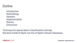
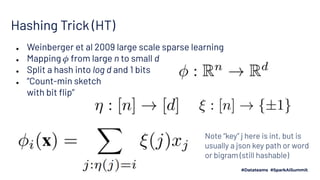
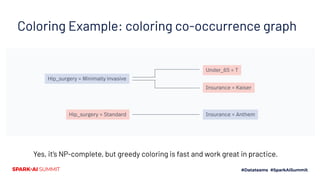
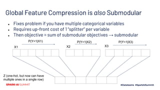
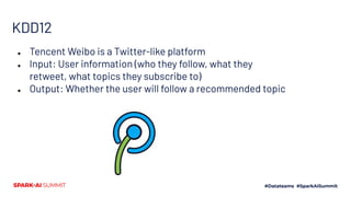
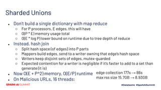
![Structures for your sparse data
● Low-width design matrix
○ Preferably 100s to 1000s of active bits per row (= “nnz”)
● Simplifications
○ Categorical → One-hot “is_CA, is_NV, …”
○ Small counts → unary one-hot “bat [1 time]” “bat [2 times]”
○ Sparse and continuous → bin, one-hot “10K-1M followers”](https://image.slidesharecdn.com/481vladfeinberg-200629025833/85/Chromatic-Sparse-Learning-7-320.jpg)
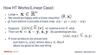

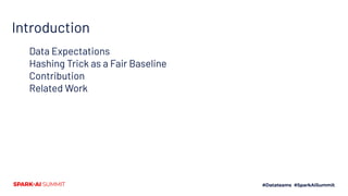
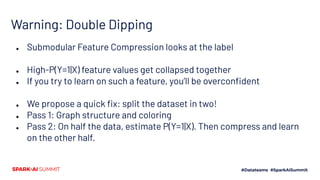
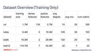
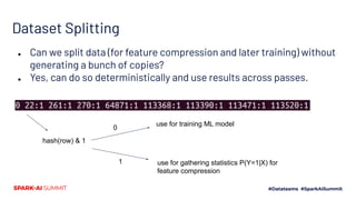
![Contribution
Use an efficient graph construction technique and graph coloring
[1] to shrink datasets from millions of sparse features to 100s of
columns.
Extend a mechanism [2] for categorical feature compression to
featurize effectively. Avoiding so-called target leakage [3] allows high
accuracy with few features.](https://image.slidesharecdn.com/481vladfeinberg-200629025833/85/Chromatic-Sparse-Learning-13-320.jpg)
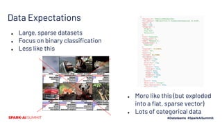
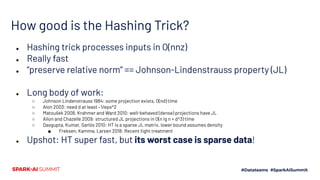
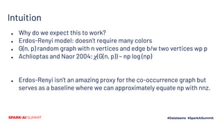
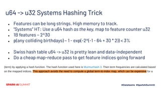
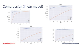
![Related Work
● Many individual lines of work are called upon, but these solve more
specific problems and can’t be applied to a general sparse binary
problem:
○ [1] Exclusive Feature Bundling from LGBM (Ke et al 2017)
○ [2] Categorical Feature Compression via Submodular Optimization (Bateni et al 2019)
○ [3] Target leakage from Catboost (Prokhorenkova et al 2018)
● Ultimately, we depend on
the chromatic number of the graph we construct
and submodularity approximations.
● As data-dependent properties
using them enables improvement over HT, which is oblivious.](https://image.slidesharecdn.com/481vladfeinberg-200629025833/85/Chromatic-Sparse-Learning-14-320.jpg)
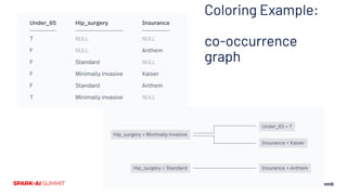
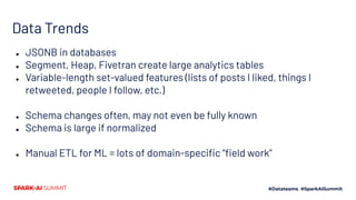
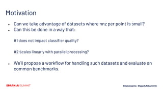
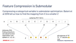
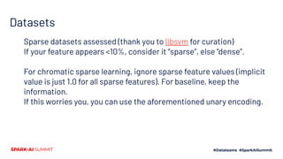
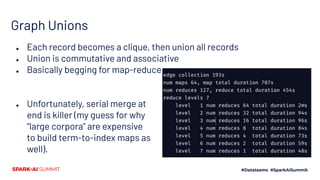
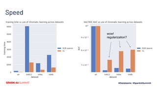
![Submodular Feature Compression
Detour to Kurkoski and Yagi 2014
View data points as a channel
Encode binary X with multivalue code Y
that “transmits” the label as a message.
But Y might take on lots (M) values. If we
quantize it into a slimmer Z with just K
values, preserve label info with
max_Z I(Z(Y) ; X) [after this slide we’ll go
back to normal lettering, Y is label]
Warning… their X and Y are
flipped from typical ML use](https://image.slidesharecdn.com/481vladfeinberg-200629025833/85/Chromatic-Sparse-Learning-22-320.jpg)
![URL
● Ma et al 2009
● Sequential data, so train on early days, predict on late [all datasets will
be like this]
● Input: lexical and host-based features of url
● Output: is this a malicious website?](https://image.slidesharecdn.com/481vladfeinberg-200629025833/85/Chromatic-Sparse-Learning-28-320.jpg)


![Top-level Implementation
● Input format: SVMlight-ish
○ newline-separated [(feature, value)] records
● Coloring
○ Each record is a co-occurence clique
○ Union these into a dataset co-occurence graph
● Color the graph (data-independent)
● Collect P(Y=1|feature)
○ Just some counts for each feature
● Run feature compression (data-independent)
● Recode data
● Note: data-independent != free
wide but sparse
chi(G)
narrow and dense](https://image.slidesharecdn.com/481vladfeinberg-200629025833/85/Chromatic-Sparse-Learning-33-320.jpg)

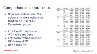
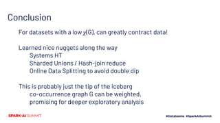

The document presents a novel approach to chromatic sparse learning, focusing on efficiently handling large, sparse datasets in binary classification by employing a graph construction and feature compression methodology. The technique leverages hashing tricks and submodular optimization to reduce dataset dimensions while maintaining classifier quality and allowing for parallel processing. Results indicate significant improvements in dataset compression, facilitating the use of smaller models on modern computational resources.


![[Paper Reading] Attention is All You Need](https://cdn.slidesharecdn.com/ss_thumbnails/reading20181228-190111054908-thumbnail.jpg?width=640&height=640&fit=bounds)


![[241]large scale search with polysemous codes](https://cdn.slidesharecdn.com/ss_thumbnails/241large-scalesearchwithpolysemouscodes-171017003327-thumbnail.jpg?width=640&height=640&fit=bounds)