Download as PDF, PPTX


![Anywhere?
• Naïve algorithm!
• for i=1..N
• for j=1..N
• M[i,j] = sim(d[i], d[j])
• prune(graph)
If we have around 1
million entities, the
calculation is way bigger
than the whole set of
tweets in a year.](https://image.slidesharecdn.com/davidmartinez-buildinggraphstodiscoverinformation-bigdataspain2015-151021092551-lva1-app6891/75/Building-graphs-to-discover-information-by-David-Martinez-at-Big-Data-Spain-2015-14-2048.jpg)
![LSH
8 Kristen Grauman and Rob Fergus
D t b
hr r
n
Database
hr1…rb
<< n
XiSeries of b
randomized LSH
functions
Colliding instances
are searched
110101
<< n
Q
functions
Q
111101
110111
hr1…rb
Hash table:
Similar instances collide, w.h.p.
Query
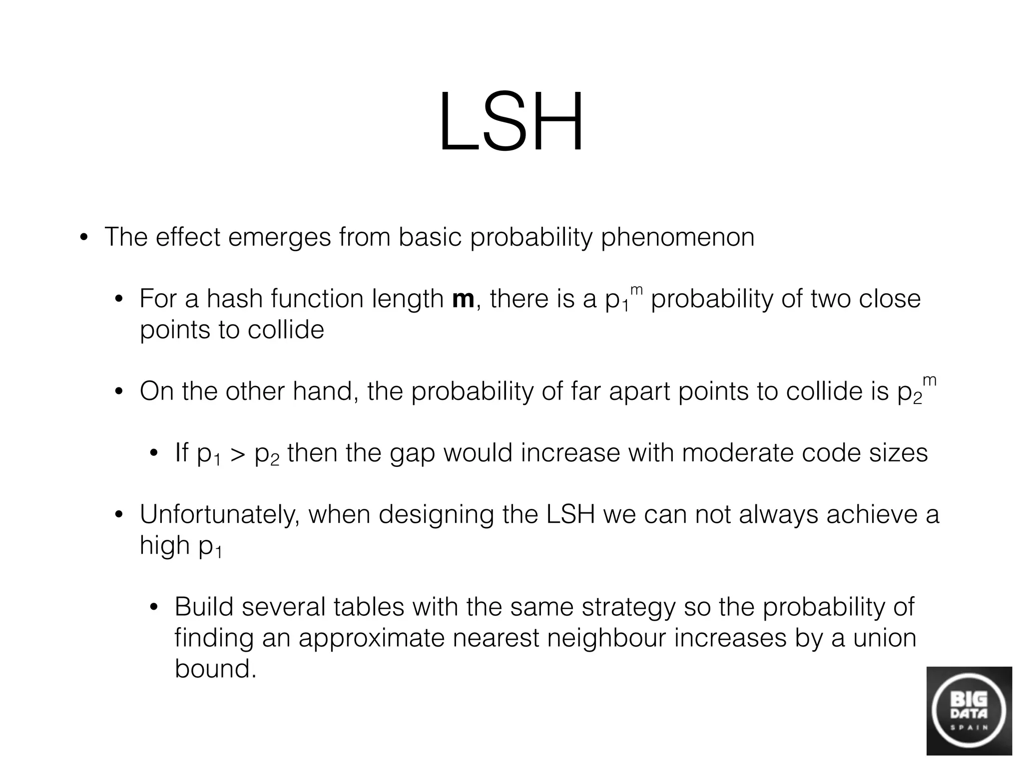
Fig. 5 Locality Sensitive Hashing (LSH) uses hash keys constructed so as to guarantee collision is
more likely for more similar examples [33, 23]. Once all database items have been hashed into the
table(s), the same randomized functions are applied to novel queries. One exhaustively searches
only those examples with which the query collides.
counters some of these shortcomings, and allows a user to explicitly control the
similarity search accuracy and search time tradeoff [23].
Kristen Grauman & Rob Fergus
Local Sensitivity Hashing](https://image.slidesharecdn.com/davidmartinez-buildinggraphstodiscoverinformation-bigdataspain2015-151021092551-lva1-app6891/75/Building-graphs-to-discover-information-by-David-Martinez-at-Big-Data-Spain-2015-16-2048.jpg)
![LSH
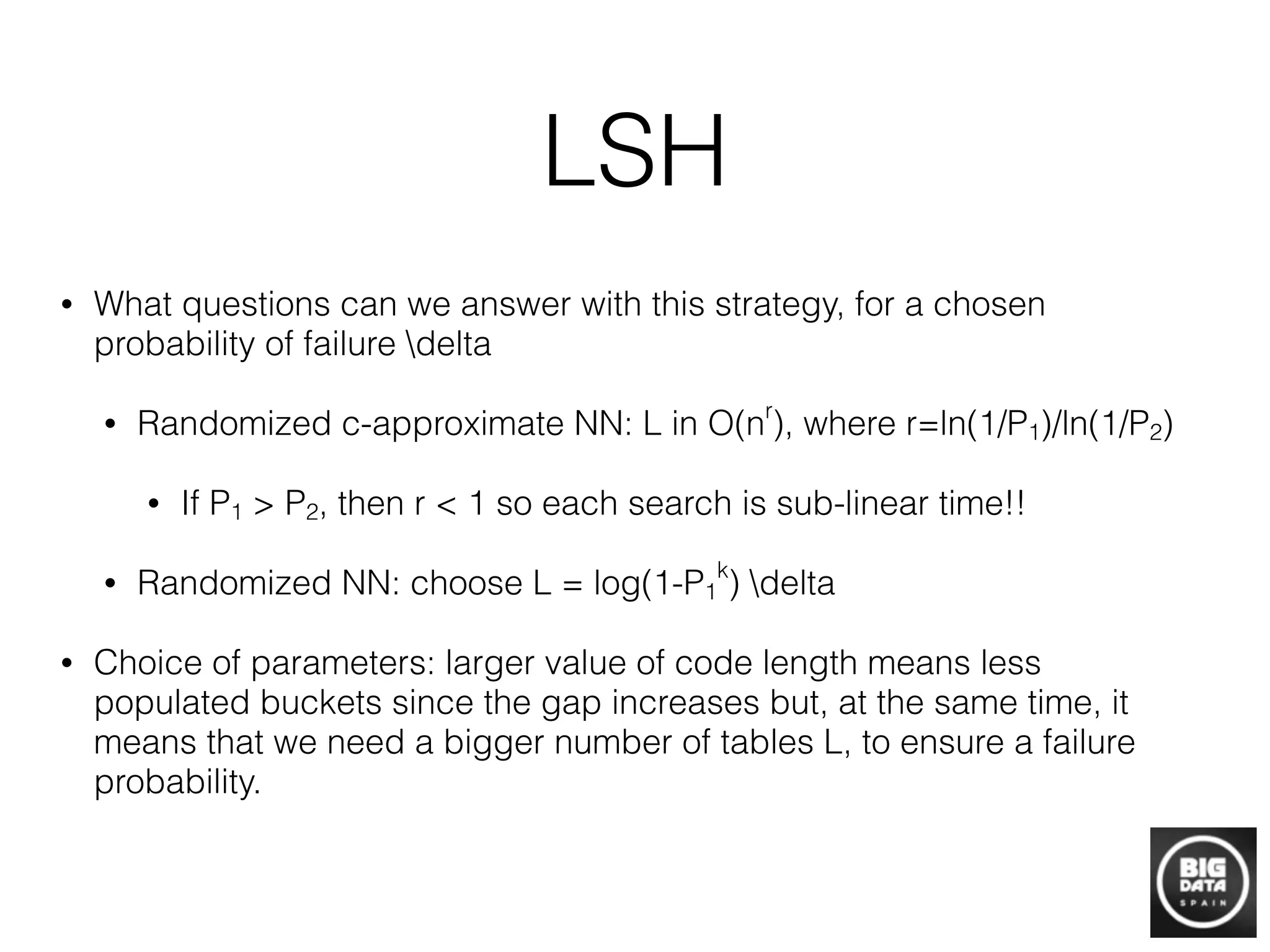
• LSH relies on the existence of LSH Family of functions
for a given metric.
• A family H is (R, cR, P1, P2)-sensitive if for any two
points p and q!
• if |p-q| < R, then P[h(p) == h(q)] > P1
• if |p-q| > cR, then P[h(p) == h(q)] < P2
where h is independently randomly selected from
family H and P1 > P2](https://image.slidesharecdn.com/davidmartinez-buildinggraphstodiscoverinformation-bigdataspain2015-151021092551-lva1-app6891/75/Building-graphs-to-discover-information-by-David-Martinez-at-Big-Data-Spain-2015-17-2048.jpg)
![LSH
input set into a bucket gj(p), for j = 1,…,L. Since the total number of
buckets may be large, we retain only the nonempty buckets by resort-
ing to (standard) hashing3
of the values gj(p). In this way, the data
structure uses only O(nL) memory cells; note that it suffices that the
buckets store the pointers to data points, not the points themselves.
To process a query q, we scan through the buckets g1(q),…, gL(q), and
retrieve the points stored in them. After retrieving the points, we com-
3
See [16] for more details on hashing.
log1 – P1
k ␦ so that (1 – P1
k)L ≤ ␦, then any R-neighbor of q is returned by
the algorithm with probability at least 1 – ␦.
How should the parameter k be chosen? Intuitively, larger values of
k lead to a larger gap between the probabilities of collision for close
points and far points; the probabilities are P1
k and P2
k, respectively (see
Figure 3 for an illustration). The benefit of this amplification is that the
hash functions are more selective. At the same time, if k is large then
P1
k is small, which means that L must be sufficiently large to ensure
that an R-near neighbor collides with the query point at least once.
Preprocessing:
1. Choose L functions gj, j = 1,…L, by setting gj = (h1, j, h2, j,…hk, j), where h1, j,…hk, j are chosen at random from the LSH family H.
2. Construct L hash tables, where, for each j = 1,…L, the jth hash table contains the dataset points hashed using the function gj.
Query algorithm for a query point q:
1. For each j = 1, 2,…L
i) Retrieve the points from the bucket gj(q) in the jth hash table.
ii) For each of the retrieved point, compute the distance from q to it, and report the point if it is a correct answer (cR-near
neighbor for Strategy 1, and R-near neighbor for Strategy 2).
iii) (optional) Stop as soon as the number of reported points is more than LЈ.
Fig. 2. Preprocessing and query algorithms of the basic LSH algorithm.
COMMUNICATIONS OF THE ACM January 2008/Vol. 51, No. 1 119](https://image.slidesharecdn.com/davidmartinez-buildinggraphstodiscoverinformation-bigdataspain2015-151021092551-lva1-app6891/75/Building-graphs-to-discover-information-by-David-Martinez-at-Big-Data-Spain-2015-19-2048.jpg)
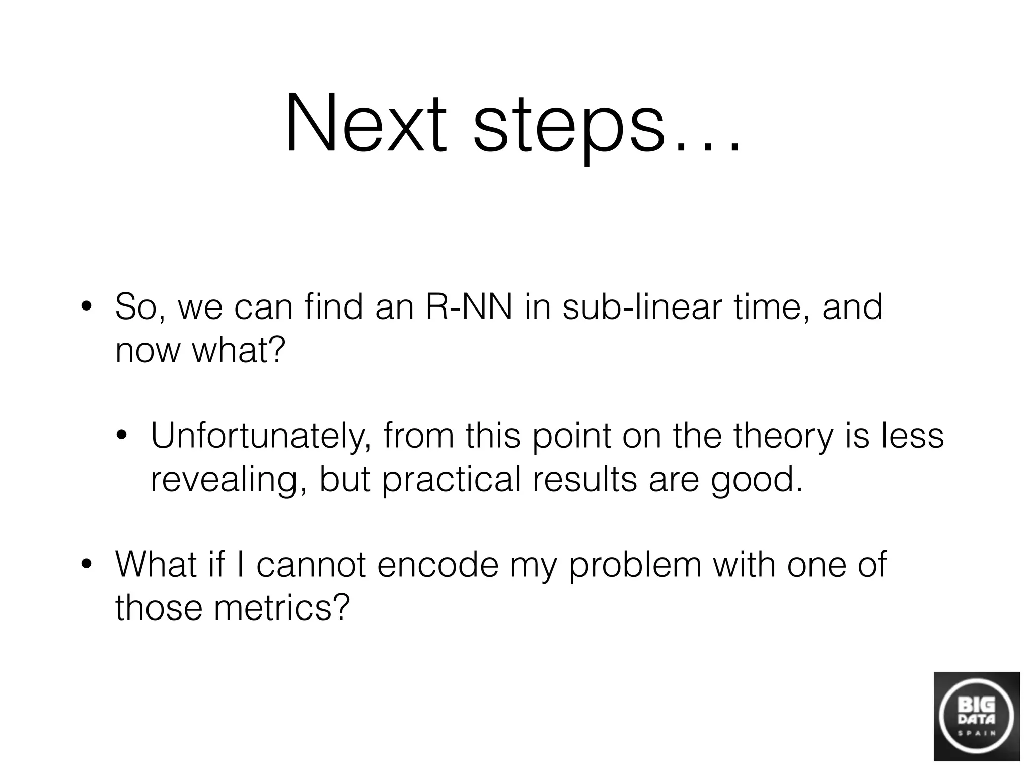
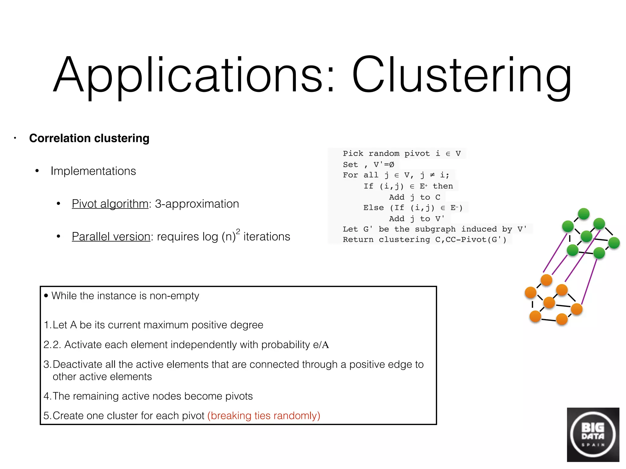
![Applications: Inference
Idea: by minimising total
variation with respect with
the most connected
neighbours, we can infer
geolocation for twitter users.
See: Geotagging One Hundred Million
Twitter Accounts with Total Variation
Minimization. IEEE 2014 Conference on
Big Data
Figure 6: Histogram of tweets as a function of activity level.
For each group of users described in fig. 4 and fig. 5 we
collected the total number of tweets generated by the group.
Despite the high number of inactive users, the bulk of tweets
are generated by active Twitter users, indicating the impor-
tance of geotagging active accounts.
Figure 7: Histogram of errors with di↵erent restrictions on
the maximum allowable geographic dispersion of each user’s
(a) CDF of the geographic distance between friends (b) CDF of the geographic distance between a user and their
geographically closest friend
Figure 2: Study of contact patterns between users who reveal their location via GPS. Subgraphs of GPS users are taken
from the, the bidirectional @mention network (blue), bidirectional @mention network after filtering edges for triadic closures
(green), and the complete unidirectional @mention network (black). In (a), we see that the distances spanned by reciprocated
@mentions (blue and green) are smaller than those spanned by any @mention (black). In (b), we see that users often have
at least one online social tie with a geographically nearby user. The subgraph sizes are: 19,515,278 edges and 3,972,321
nodes (green), 20,576,189 edges and 4,488,759 node (blue), 100,126,247 edges and 5,648,220 nodes (black). We suspect
these results would be even stronger if more GPS data were available.
well-aligned with geographic distance, we restrict our atten-
tion to GPS-known users and study contact patterns between
them in fig. 2.
Users with GPS-known locations make up only a tiny por-
tion of our @mention networks. Despite the relatively small
amount of data, we can still see in fig. 2 that online social
ties typically form between users who live near each other
and that a majority of GPS-known users have at least one
GPS-known friend within 10km.
The optimization (1) models proximity of connected users.
Unfortunately, the total variation functional is nondi↵eren-
tiable and finding a global minimum is thus a formidable chal-
lenge. We will employ “parallel coordinate descent” [25] to
solve (1). Most variants of coordinate descent cycle through
the domain sequentially, updating each variable and commu-
nicating back the result before the next variable can update.
The scale of our data necessitates a parallel approach, pro-
hibiting us from making all the communication steps required
by a traditional coordinate descent method.
At each iteration, our algorithm simultaneously updates
each user’s location with the l1-multivariate median of their
friend’s locations. Only after all updates are complete do we
communicate our results over the network.
At iteration k, denote the user estimates by fk
and the
variation on the ith node by
∇i(fk
,f) =
j
wijd(f,fk
j ) (6)
Parallel coordinate descent can now be stated concisely in alg.
1.
The argument that minimizes (6) is the l1-multivariate me-
dian of the locations of the neighbours of node i. By placing
this computation inside the parfor of alg. 1, we have repro-
duced the Spatial Label Propagation algorithm of [12] as a
Algorithm 1: Parallel coordinate descent for constrained
TV minimization
Initialize: fi = li for i ∈ L
for k = 1...N do
parfor i :
if i ∈ L then
fk+1
i = li
else
fk+1
i = argmin
f
∇i(fk
,f)
end
end
fk
= fk+1
end
coordinate descent method designed to minimize total varia-
tion.
3.4 Individual Error Estimation
The vast majority of Twitter users @mention with geograph-
ically close users. However, there do exist several users who
have amassed friends dispersed around the globe. For these
users, our approach should not be used to infer location.
We use a robust estimate of the dispersion of each user’s
friend locations to infer accuracy of our geocoding algorithm.
Our estimate for the error on user i is the median absolute
deviation of the inferred locations of user i’s friends, com-
puted via (3). With a dispersion restriction as an additional
parameter, , our optimization becomes
min
f
∇f subject to fi = li for i ∈ L and max
i
∼
∇fi (7)](https://image.slidesharecdn.com/davidmartinez-buildinggraphstodiscoverinformation-bigdataspain2015-151021092551-lva1-app6891/75/Building-graphs-to-discover-information-by-David-Martinez-at-Big-Data-Spain-2015-29-2048.jpg)
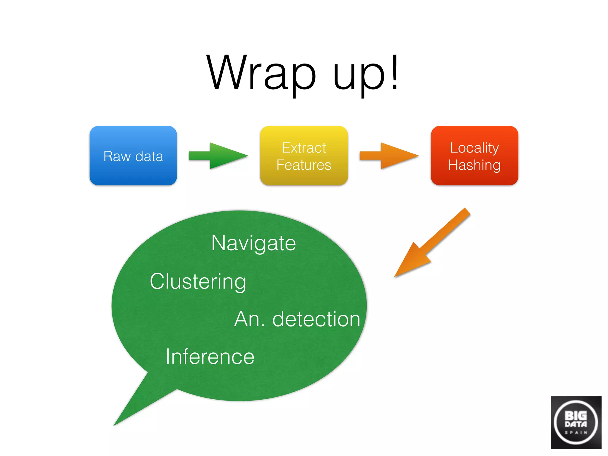


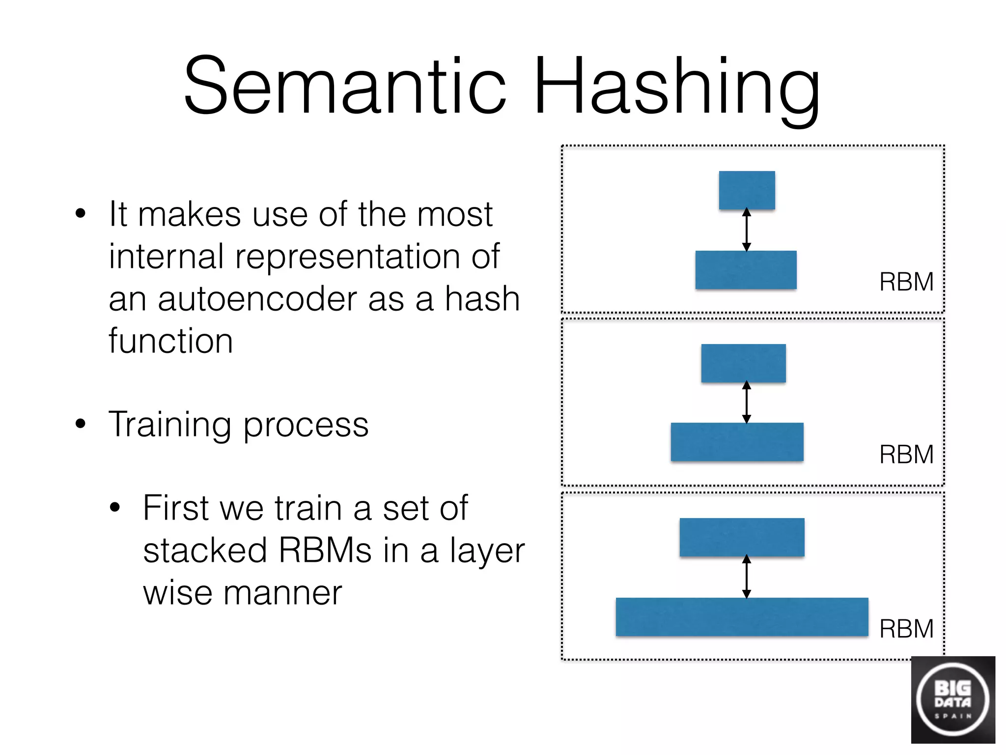
Graphs can be built from raw data to discover information by representing relationships between data points as graph connections. Techniques like locality sensitive hashing can be used to efficiently construct graphs from high-dimensional data by mapping similar points to the same "buckets". Once a graph is built, algorithms can find structure like connected components, detect anomalies using local outlier factor, perform clustering, and make inferences about unlabeled nodes. Building graphs is a powerful approach for transforming raw data into useful information through network analysis and machine learning on graphs.


![Coded Agents – with UiPath SDK + LangGraph [Virtual Hands-on Workshop]](https://cdn.slidesharecdn.com/ss_thumbnails/codedagentsdeck-251215155422-5497c599-thumbnail.jpg?width=640&height=640&fit=bounds)


