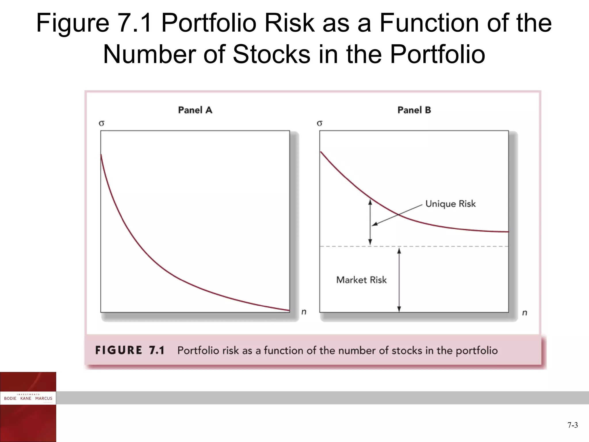
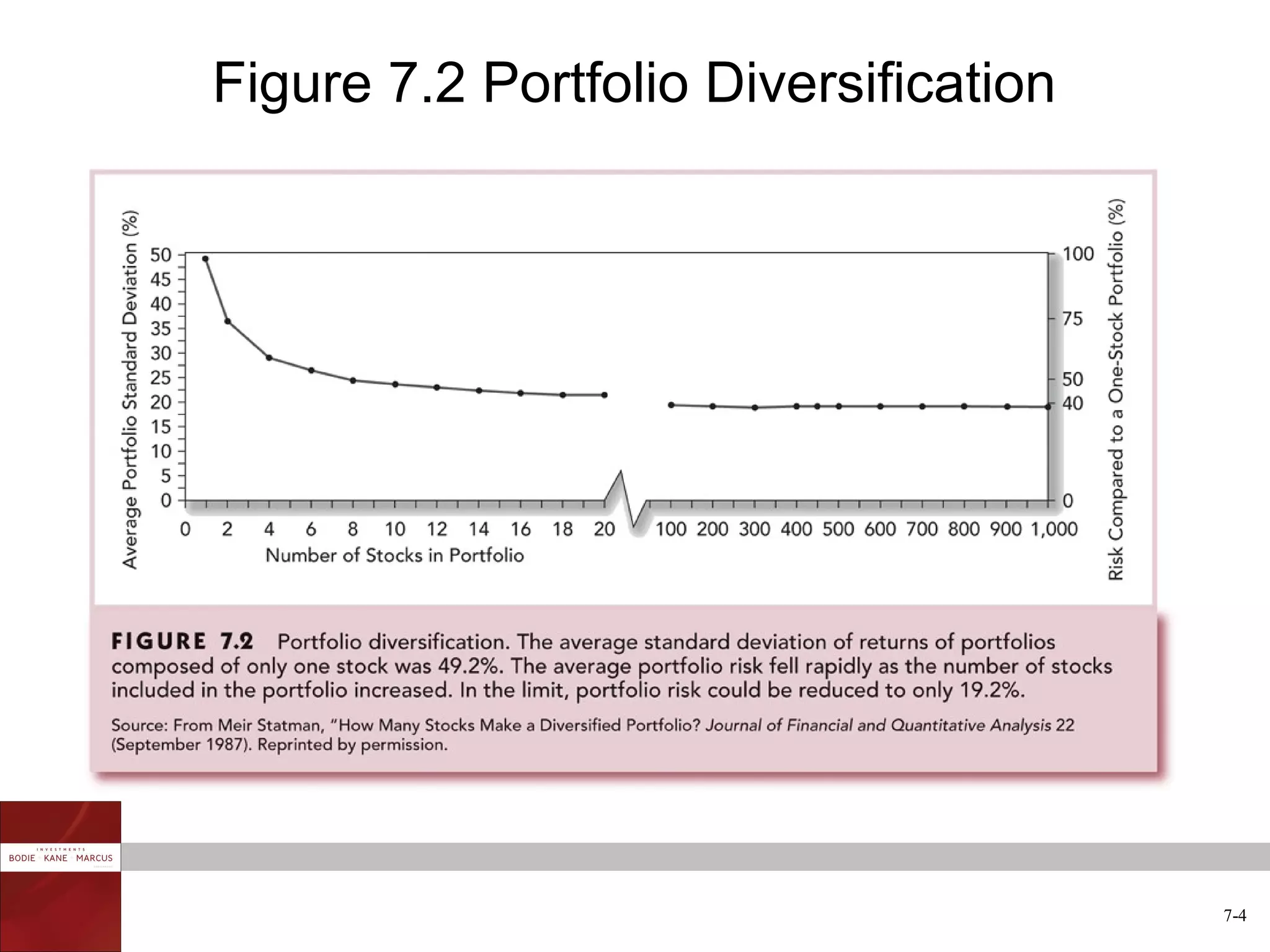
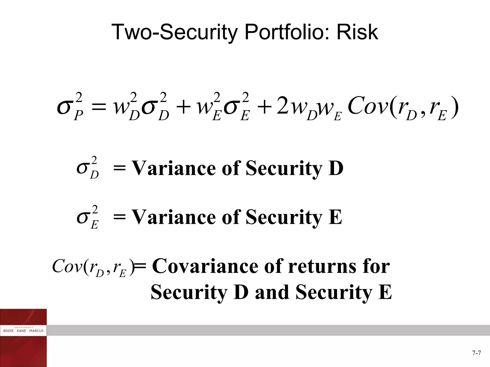
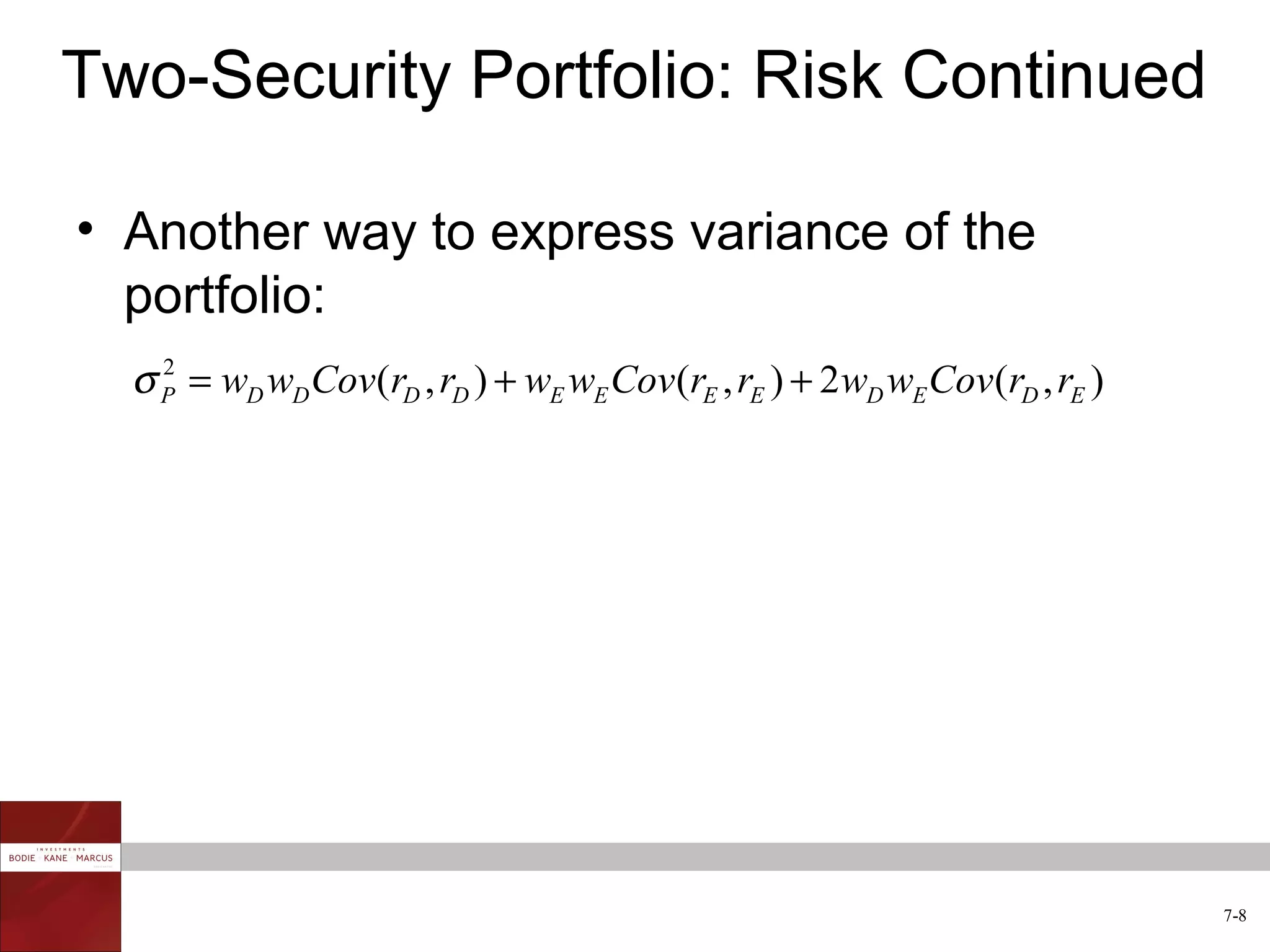
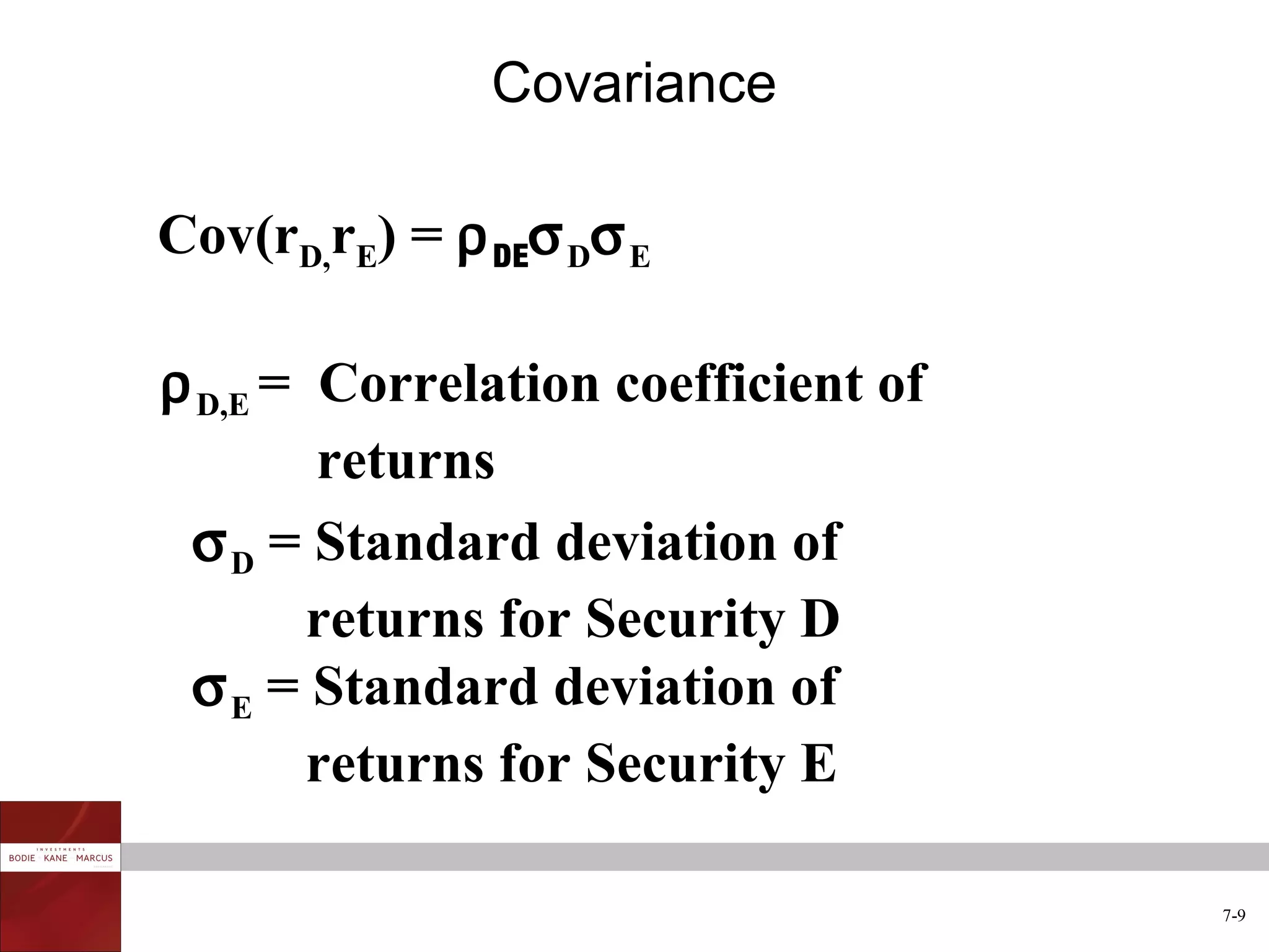
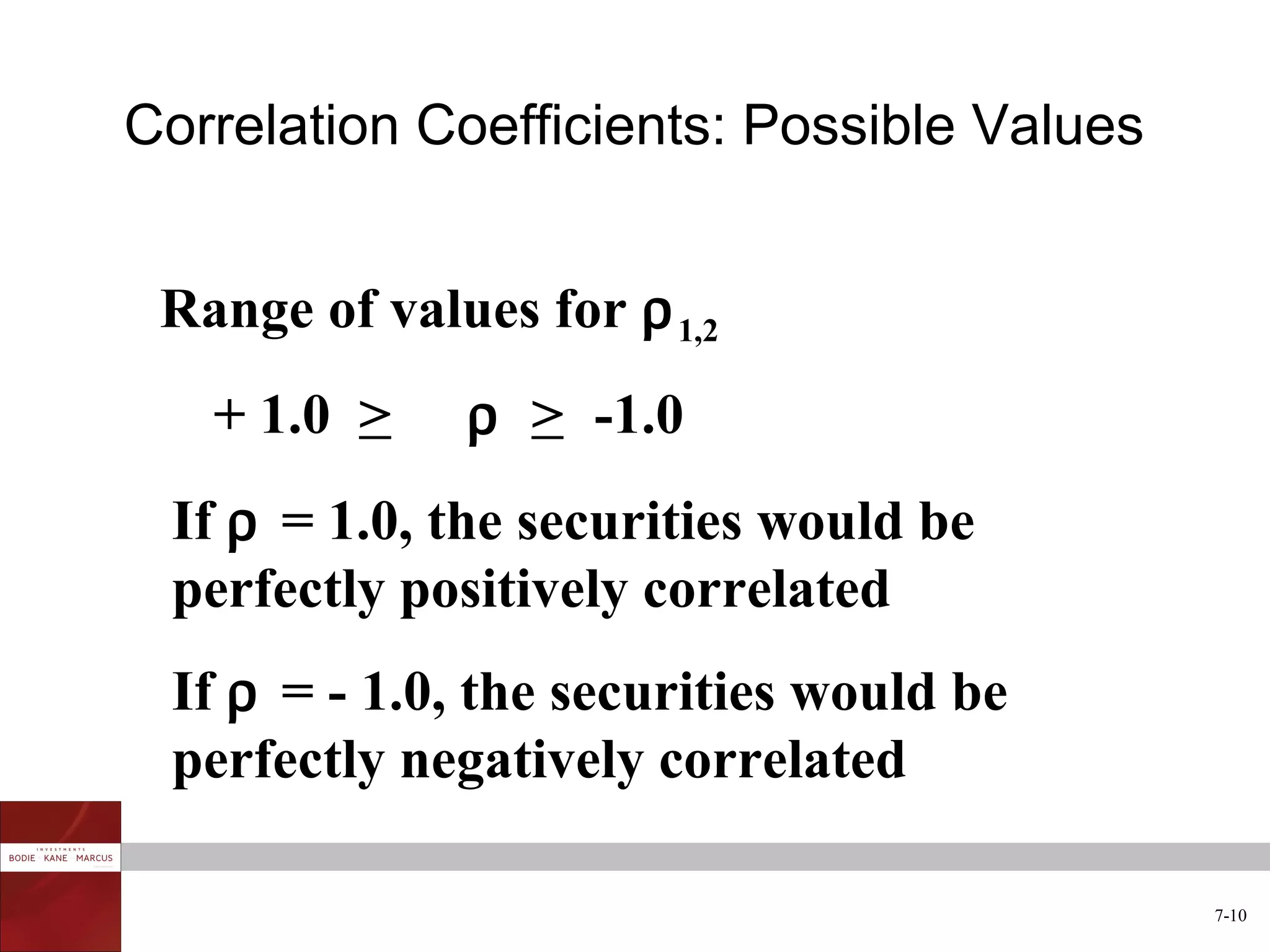
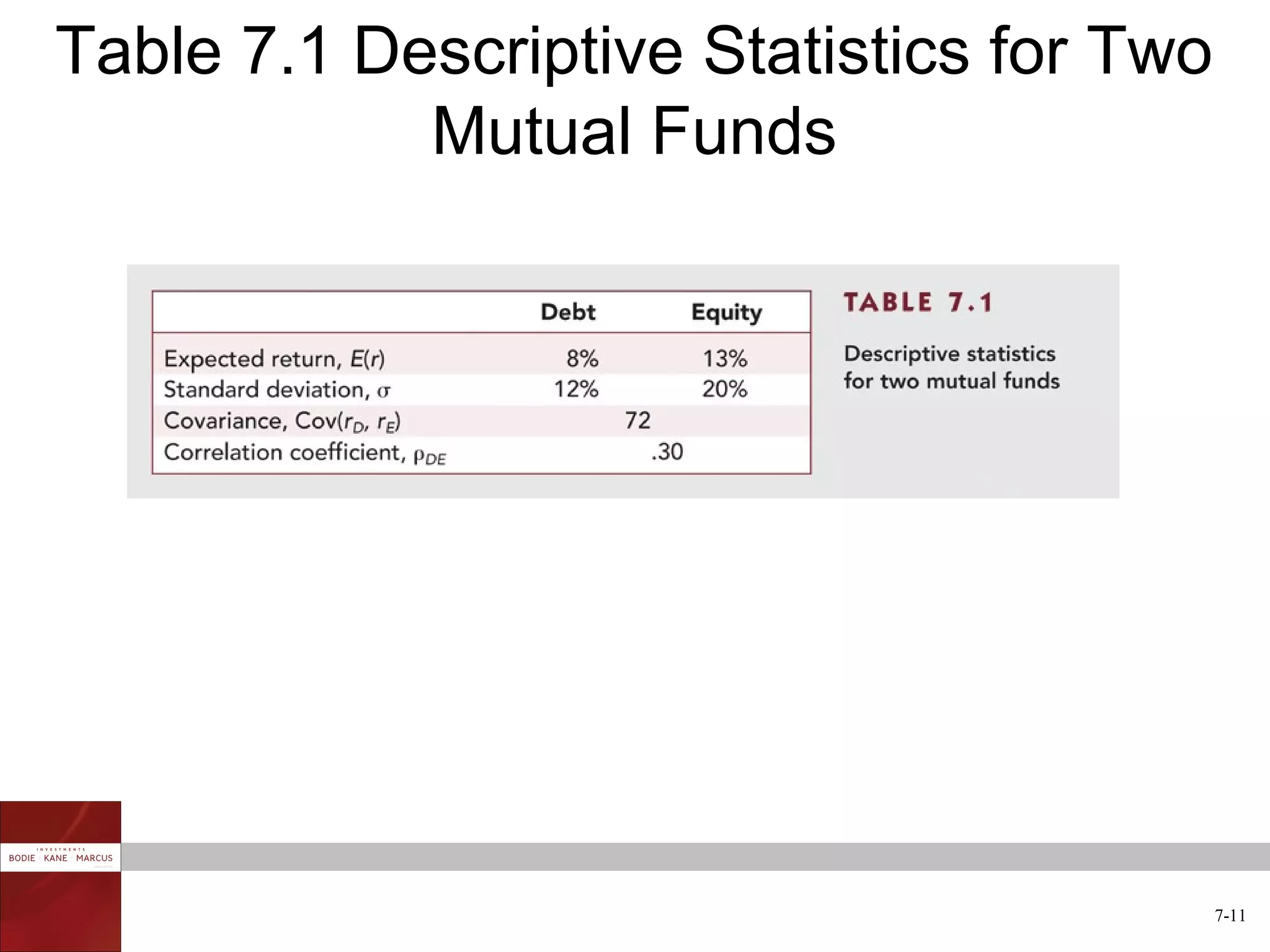
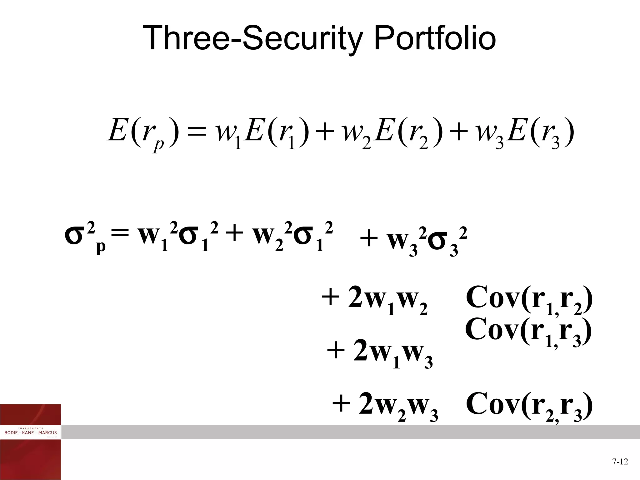
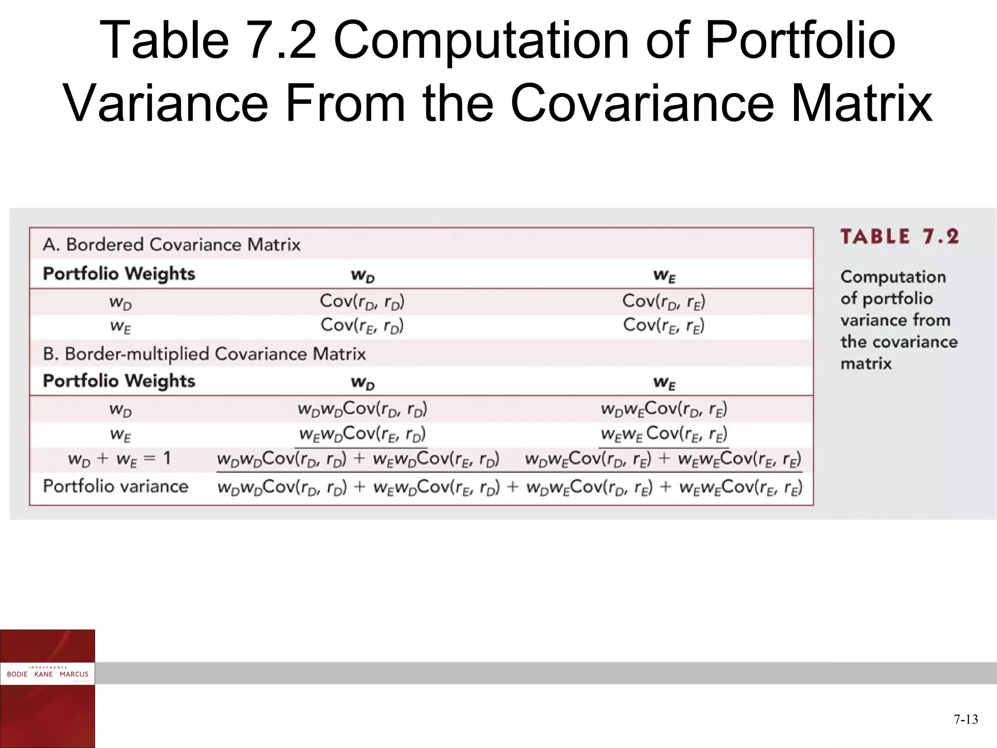
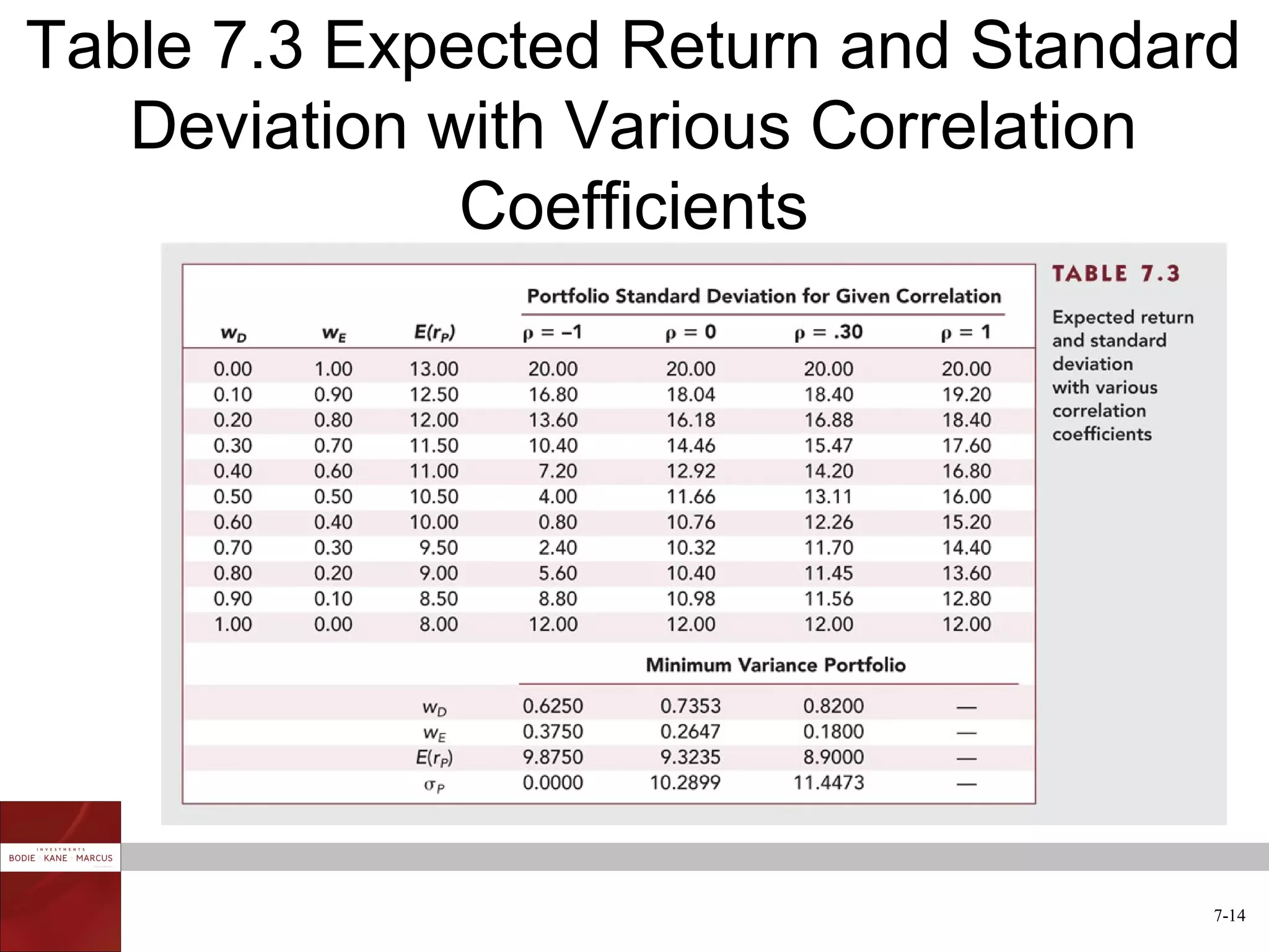
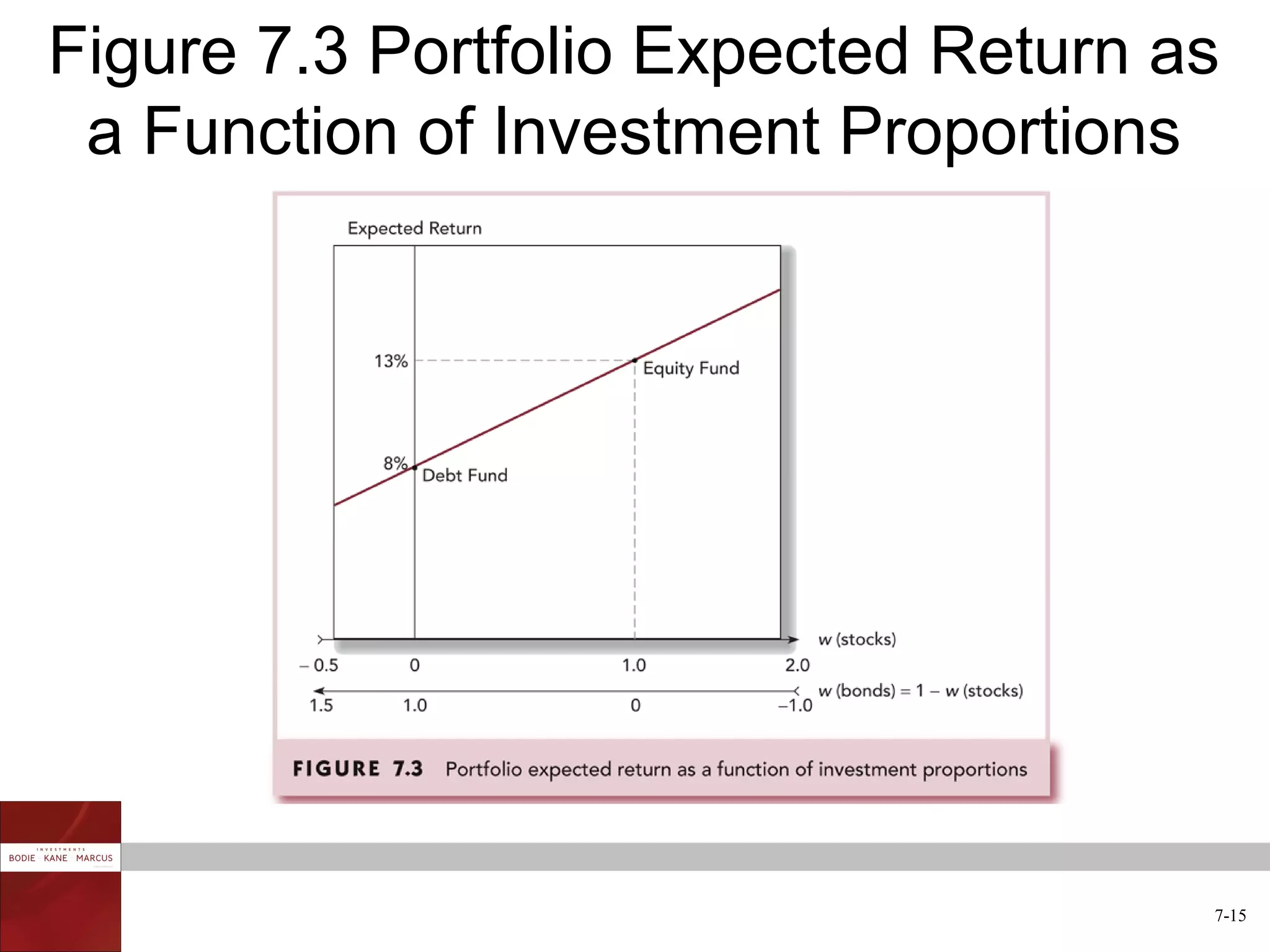
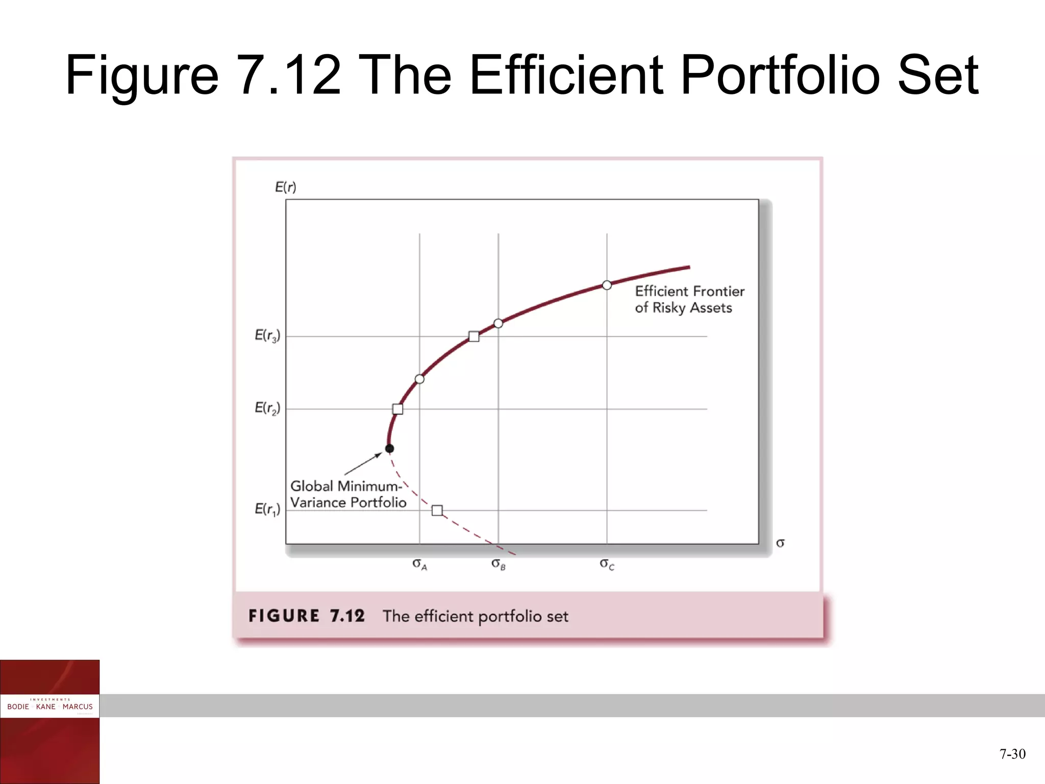
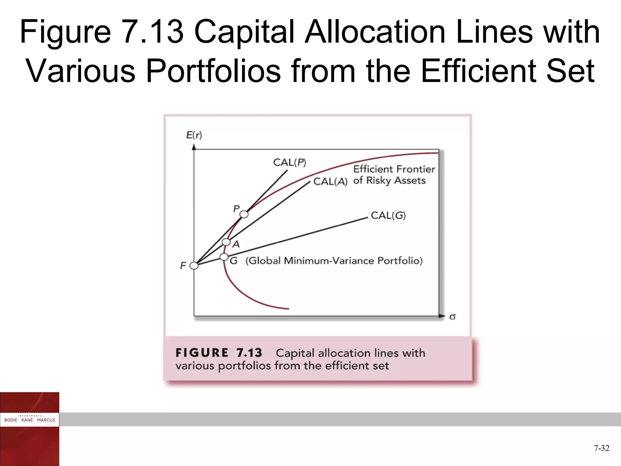
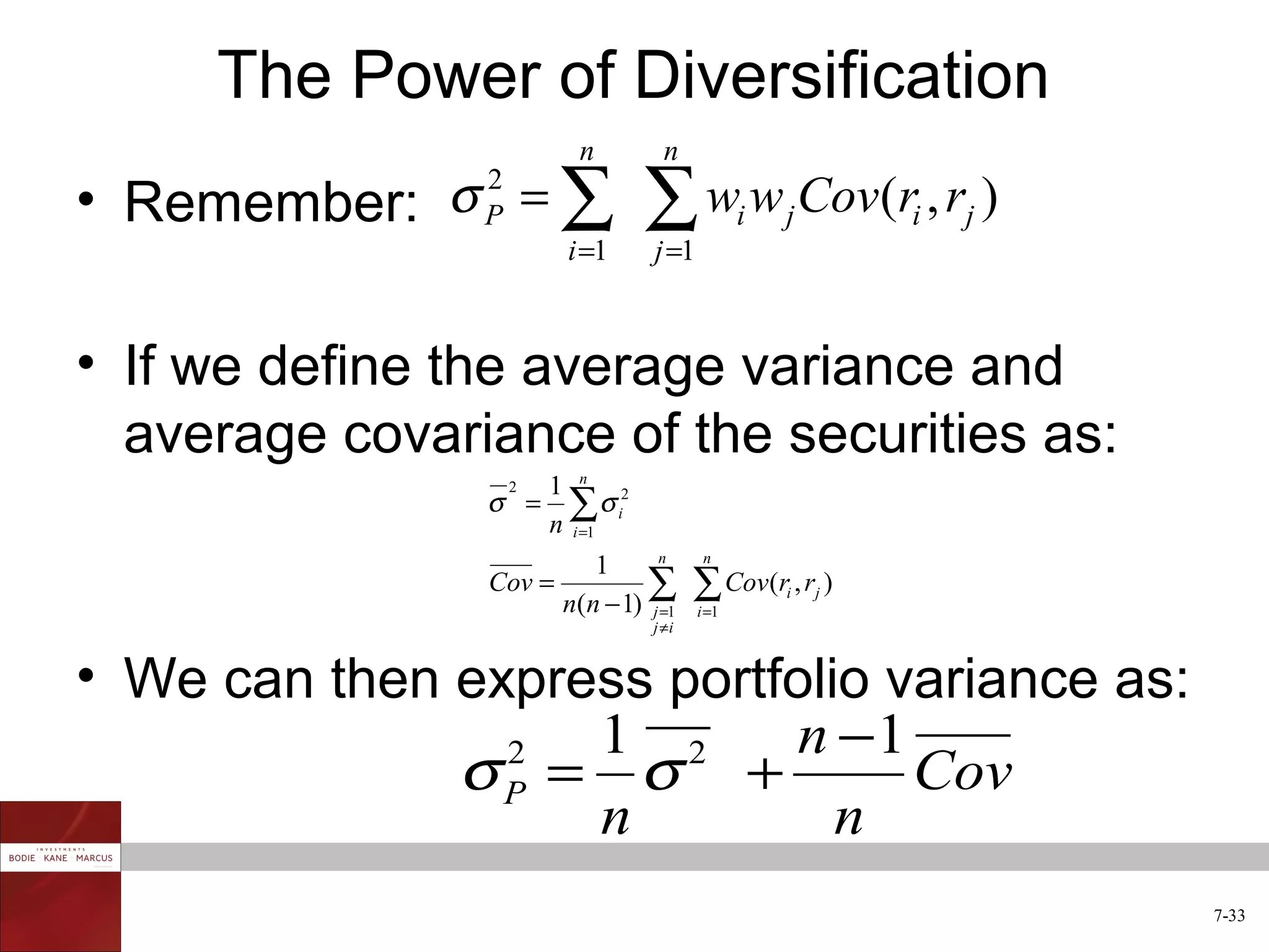
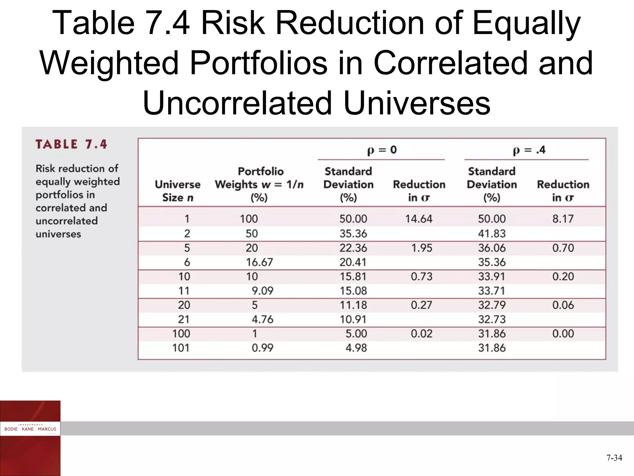
The document discusses optimal risky portfolios and diversification. It covers how portfolio risk depends on the correlation between asset returns, how to calculate portfolio variance and risk for two and three asset portfolios, the benefits of diversification in reducing risk, and how to construct efficient portfolios using the Markowitz model. The key benefits of diversification are reducing non-systematic risk and obtaining portfolios on the efficient frontier with higher risk-adjusted returns.

1. CHAPTER 7 Optimal Risky
Portfolios
Investments, 8th edition
Bodie, Kane and Marcus
Slides by Susan Hine
McGraw-Hill/Irwin Copyright © 2009 by The McGraw-Hill Companies, Inc. All rights reserved.

2. Diversification and Portfolio Risk
• Market risk
– Systematic or nondiversifiable
• Firm-specific risk
– Diversifiable or nonsystematic
7-2

3. Figure 7.1 Portfolio Risk as a Function of the
Number of Stocks in the Portfolio
7-3

4. Figure 7.2 Portfolio Diversification
7-4

5. Covariance and Correlation
• Portfolio risk depends on the correlation
between the returns of the assets in the
portfolio
• Covariance and the correlation coefficient
provide a measure of the way returns two
assets vary
7-5

6. Two-Security Portfolio: Return
rp = wr
D D
+ wEr E
rP = Portfolio Return
wD = Bond Weight
rD = Bond Return
wE = Equity Weight
rE = Equity Return
E (rp ) = wD E (rD ) + wE E (rE )
7-6

7. Two-Security Portfolio: Risk
σ = w σ + w σ + 2wDwE Cov(rD , rE )
2
P
2
D
2
D σE2
E
2
E
σ D = Variance of Security D
2
σ 2
E = Variance of Security E
Cov(rD , rE )= Covariance of returns for
Security D and Security E
7-7

8. Two-Security Portfolio: Risk Continued
• Another way to express variance of the
portfolio:
σ P = wD wD Cov(rD , rD ) + wE wE Cov (rE , rE ) + 2wD wE Cov (rD , rE )
2
7-8

9. Covariance
Cov(rD,rE) = ρ DEσ Dσ E
ρ D,E = Correlation coefficient of
returns
σ D = Standard deviation of
returns for Security D
σ E = Standard deviation of
returns for Security E
7-9

10. Correlation Coefficients: Possible Values
Range of values for ρ 1,2
+ 1.0 > ρ > -1.0
If ρ = 1.0, the securities would be
perfectly positively correlated
If ρ = - 1.0, the securities would be
perfectly negatively correlated
7-10

11. Table 7.1 Descriptive Statistics for Two
Mutual Funds
7-11

12. Three-Security Portfolio
E (rp ) = w1 E (r1 ) + w2 E (r2 ) + w3 E (r3 )
σ 2p = w12σ 12 + w22σ 12 + w32σ 32
+ 2w1w2 Cov(r1,r2)
Cov(r1,r3)
+ 2w1w3
+ 2w2w3 Cov(r2,r3)
7-12

13. Table 7.2 Computation of Portfolio
Variance From the Covariance Matrix
7-13

14. Table 7.3 Expected Return and Standard
Deviation with Various Correlation
Coefficients
7-14

15. Figure 7.3 Portfolio Expected Return as
a Function of Investment Proportions
7-15

16. Figure 7.4 Portfolio Standard Deviation
as a Function of Investment Proportions
7-16

17. Minimum Variance Portfolio as Depicted
in Figure 7.4
• Standard deviation is smaller than that of
either of the individual component assets
• Figure 7.3 and 7.4 combined demonstrate the
relationship between portfolio risk
7-17

18. Figure 7.5 Portfolio Expected Return as
a Function of Standard Deviation
7-18

19. Correlation Effects
• The relationship depends on the correlation
coefficient
• -1.0 < ρ < +1.0
• The smaller the correlation, the greater the
risk reduction potential
• If ρ = +1.0, no risk reduction is possible
7-19

20. Figure 7.6 The Opportunity Set of the
Debt and Equity Funds and Two
Feasible CALs
7-20

21. The Sharpe Ratio
• Maximize the slope of the CAL for any
possible portfolio, p
• The objective function is the slope:
E (rP ) − rf
SP =
σP
7-21

22. Figure 7.7 The Opportunity Set of the
Debt and Equity Funds with the Optimal
CAL and the Optimal Risky Portfolio
7-22

23. Figure 7.8 Determination of the Optimal
Overall Portfolio
7-23

24. Figure 7.9 The Proportions of the
Optimal Overall Portfolio
7-24

25. Markowitz Portfolio Selection Model
• Security Selection
– First step is to determine the risk-return
opportunities available
– All portfolios that lie on the minimum-
variance frontier from the global minimum-
variance portfolio and upward provide the
best risk-return combinations
7-25

26. Figure 7.10 The Minimum-Variance
Frontier of Risky Assets
7-26

27. Markowitz Portfolio Selection Model
Continued
• We now search for the CAL with the highest
reward-to-variability ratio
7-27

28. Figure 7.11 The Efficient Frontier of
Risky Assets with the Optimal CAL
7-28

29. Markowitz Portfolio Selection Model
Continued
• Now the individual chooses the appropriate
mix between the optimal risky portfolio P and
T-bills as in Figure 7.8
n n
σP = ∑
2
∑ w w Cov(r , r )
i j i j
i =1 j =1
7-29

30. Figure 7.12 The Efficient Portfolio Set
7-30

31. Capital Allocation and the Separation
Property
• The separation property tells us that the
portfolio choice problem may be separated
into two independent tasks
– Determination of the optimal risky portfolio
is purely technical
– Allocation of the complete portfolio to T-
bills versus the risky portfolio depends on
personal preference
7-31

32. Figure 7.13 Capital Allocation Lines with
Various Portfolios from the Efficient Set
7-32

33. The Power of Diversification
n n
• Remember: σ = ∑ ∑ w w Cov(r , r )
2
P i j i j
i =1 j =1
• If we define the average variance and
average covariance of the securities as:
1 n 2
σ = ∑σ i
2
n i =1
n n
1
Cov = ∑
n(n − 1) j =1
∑ Cov(r , r )
i =1
i j
j ≠i
• We can then express portfolio variance as:
1 2 n −1
σP = σ +
2
Cov
n n
7-33

34. Table 7.4 Risk Reduction of Equally
Weighted Portfolios in Correlated and
Uncorrelated Universes
7-34

35. Risk Pooling, Risk Sharing and Risk in
the Long Run
• Consider the following:
Loss: payout = $100,000
p = .001
No Loss: payout = 0
1 − p = .999
7-35

36. Risk Pooling and the Insurance Principle
• Consider the variance of the portfolio:
1 2
σ = σ
2
P
n
• It seems that selling more policies causes
risk to fall
• Flaw is similar to the idea that long-term
stock investment is less risky
7-36

37. Risk Pooling and the Insurance Principle
Continued
• When we combine n uncorrelated
insurance policies each with an expected
profit of $ π, both expected total profit and
SD grow in direct proportion to n:
E (nπ ) = nE (π )
Var (nπ ) = n Var (π ) = n σ
2 2 2
SD(nπ ) = nσ
7-37

38. Risk Sharing
• What does explain the insurance business?
– Risk sharing or the distribution of a fixed
amount of risk among many investors
7-38