Downloaded 107 times

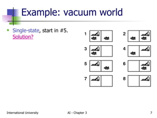
![Example: vacuum world Single-state , start in #5. Solution? [Right, Suck] Sensorless, start in { 1,2,3,4,5,6,7,8 } e.g., Right goes to { 2,4,6,8 } Solution?](https://image.slidesharecdn.com/chapter3search-1215104321871474-9/85/Chapter3-Search-8-320.jpg)
![Example: vacuum world Sensorless, start in { 1,2,3,4,5,6,7,8 } e.g., Right goes to { 2,4,6,8 } Solution? [Right,Suck,Left,Suck] Contingency Nondeterministic: Suck may dirty a clean carpet Partially observable: location, dirt at current location. Percept: [L, Clean], i.e., start in #5 or #7 Solution?](https://image.slidesharecdn.com/chapter3search-1215104321871474-9/85/Chapter3-Search-9-320.jpg)
![Example: vacuum world Sensorless, start in { 1,2,3,4,5,6,7,8 } e.g., Right goes to { 2,4,6,8 } Solution? [Right,Suck,Left,Suck] Contingency Nondeterministic: Suck may dirty a clean carpet Partially observable: location, dirt at current location. Percept: [L, Clean], i.e., start in #5 or #7 Solution? [Right, if dirt then Suck]](https://image.slidesharecdn.com/chapter3search-1215104321871474-9/85/Chapter3-Search-10-320.jpg)
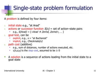
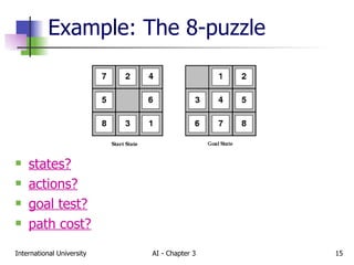
![Example: The 8-puzzle states? locations of tiles actions? move blank left, right, up, down goal test? = goal state (given) path cost? 1 per move [Note: optimal solution of n -Puzzle family is NP-hard]](https://image.slidesharecdn.com/chapter3search-1215104321871474-9/85/Chapter3-Search-16-320.jpg)
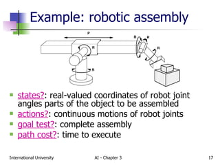
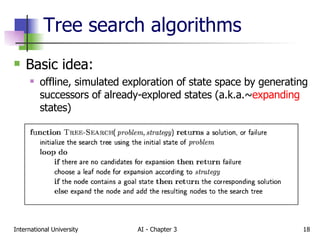
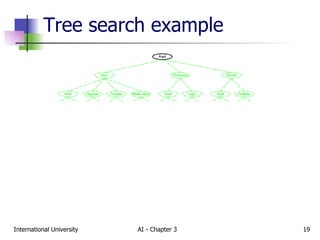
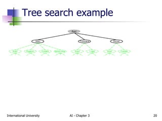
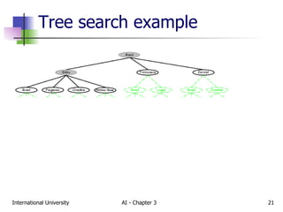
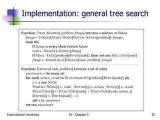
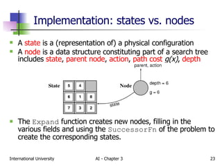
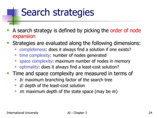
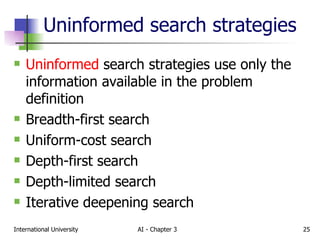
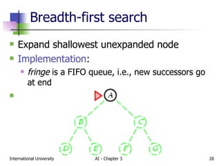
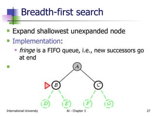
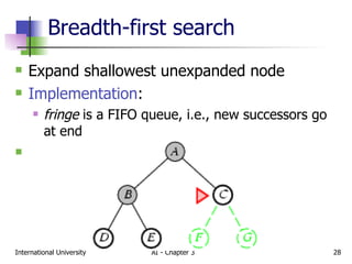
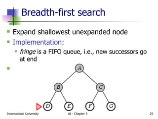
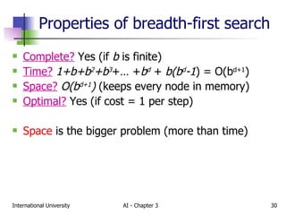
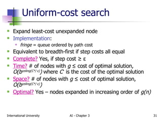
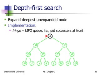
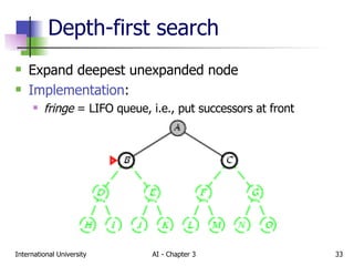
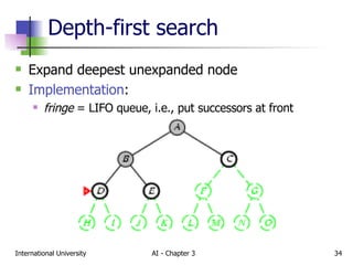
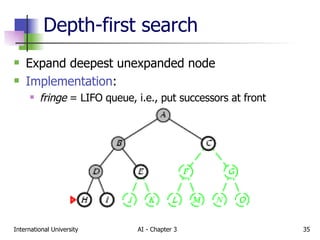
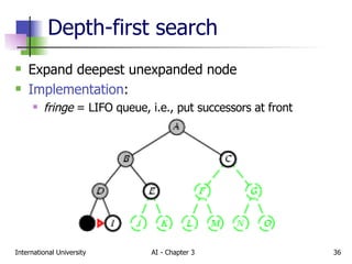
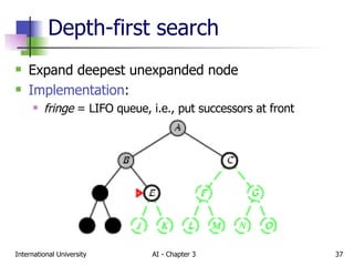
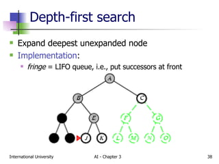
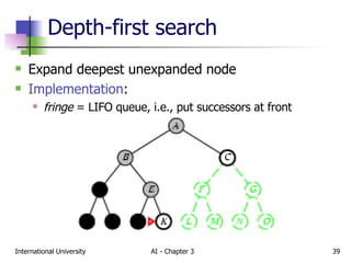
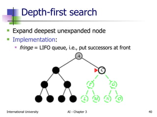
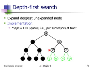
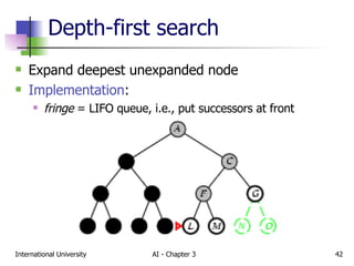
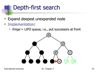
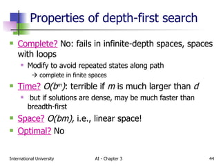
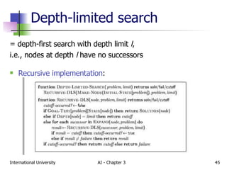
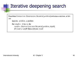
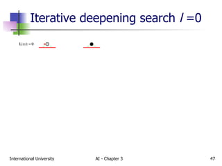
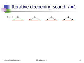
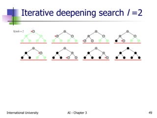
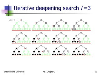
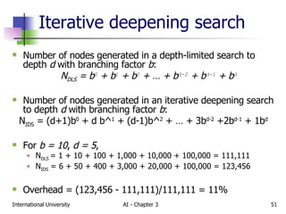
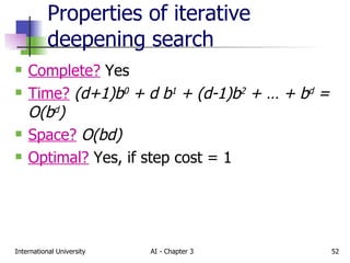
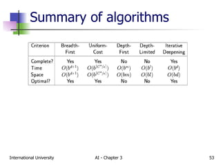

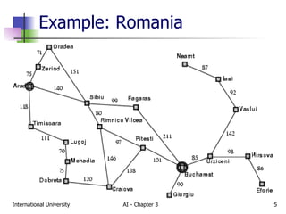
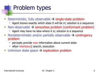
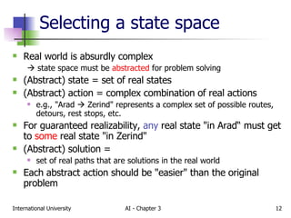
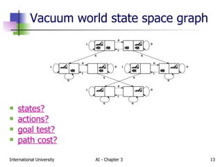
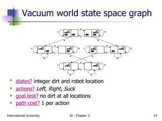
The document discusses different types of problem-solving agents and search algorithms. It describes single-state, sensorless, contingency, and exploration problem types. It also summarizes common uninformed search strategies like breadth-first search, uniform-cost search, depth-first search, depth-limited search, and iterative deepening search and analyzes their properties in terms of completeness, time complexity, space complexity, and optimality. Examples of problems that can be modeled as state space searches are also provided, like the vacuum world, 8-puzzle, and robotic assembly problems.