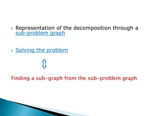
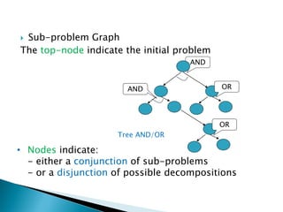
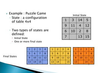
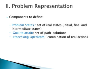
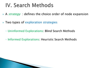
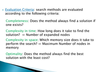
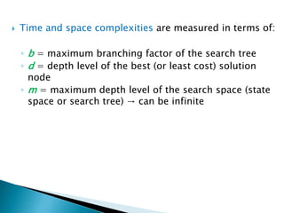
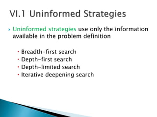
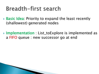
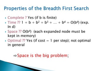
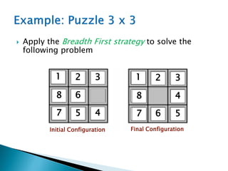
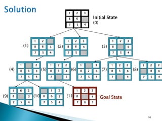
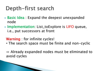
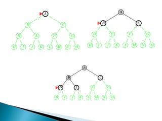
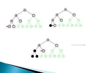
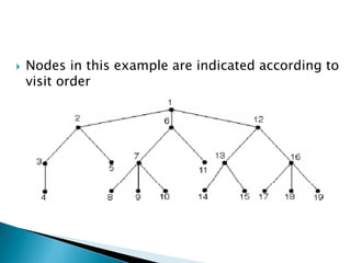
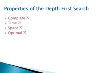
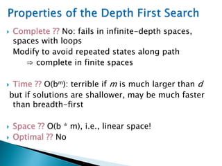
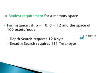
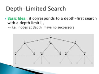
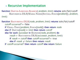
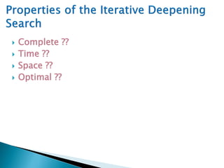
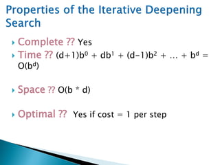
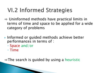
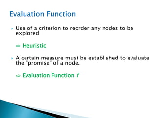
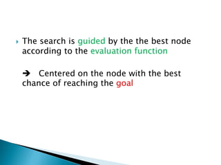
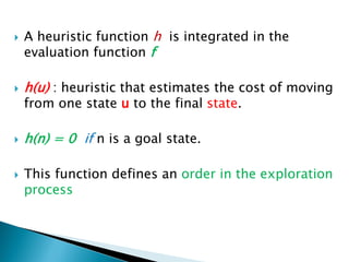
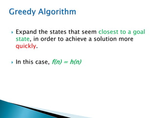
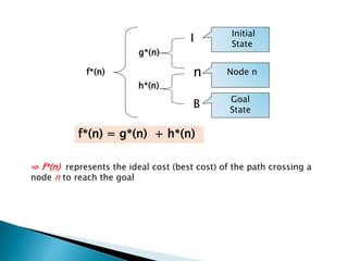
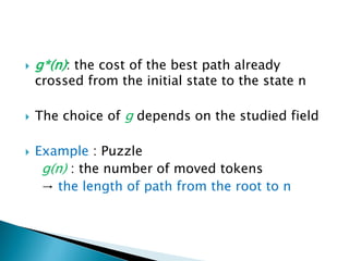
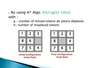
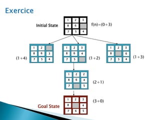
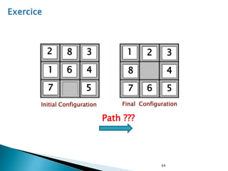
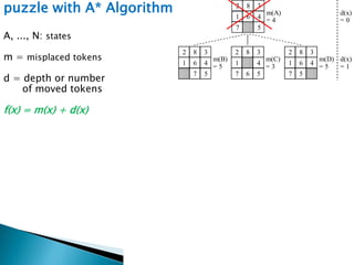
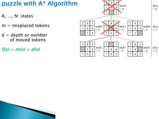
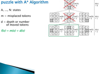
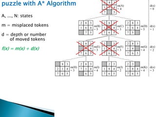
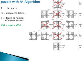
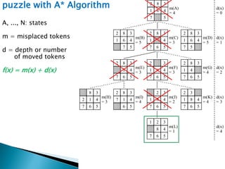
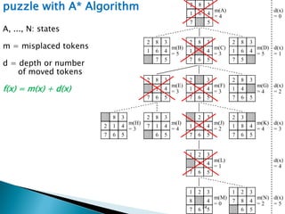
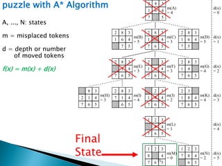
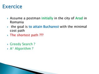
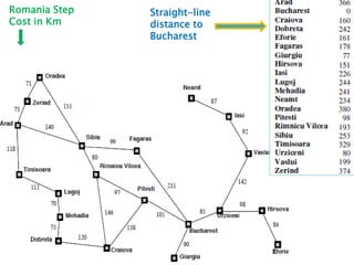
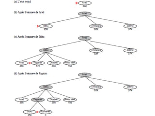
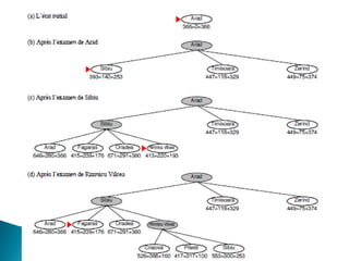
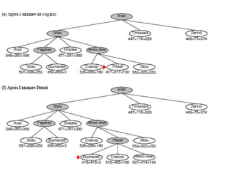
The document describes search algorithms for problem solving. It defines key concepts like state, node, problem representation, and search strategies. It then explains blind search algorithms like breadth-first search, depth-first search, depth-limited search, and iterative deepening search. Finally, it covers heuristic search algorithms like greedy search and A* search, which use an evaluation function and heuristic to guide the search towards more promising solutions.

1. Dr. Imen Boudali
Department of ICT- ENIT
imen.boudali@gmail.com
Imen.Boudali@enit.utm.tn
Chapter 2
2023-2024

2. ◦ Introduction
◦ Problem Representation
◦ State Graph
◦ Search Methods
◦ Blind Search Algorithms
◦ Heuristic Algorithms

3.  Solve a problem : Find a path from the
initial state to a final state (goal)
Initial
State
Final
State
Path??

4.  Solving Approach: Decompose the problem into
sub-problems and then break them down, etc.,
 Stop condition: Get problems with immediate
solution without decomposing them.

5.  Representation of the decomposition through a
sub-problem graph
 Solving the problem
⇕
Finding a sub-graph from the sub-problem graph

6.  Sub-problem Graph
The top-node indicate the initial problem
AND
OR
AND
OR
Tree AND/OR
• Nodes indicate:
- either a conjunction of sub-problems
- or a disjunction of possible decompositions

7.  Example : Puzzle Game
◦ State : a configuration
of table 4x4
◦ Two types of states are
defined:
 Initial State
 One or more final state
1 3 14 5
9 11 4 12
6 10 2 8
7 13 15
Initial State
7
1 2 3 4
5 6 7 8
9 10 11 12
13 14 15
1 2 3 4
5 6 7 8
9 10 11 12
13 14 15
1 2 3 4
5 6 7 8
9 10 11 12
13 14 15
Final States

8.  Components to define:
• Problem States : set of real states (initial, final and
intermediate states)
• Goal to attain: set of path-solutions
• Processing Operators : combination of real actions

9. 4 Elements to specify:
◦ Initial state
◦ operators (or succeeding_function S(x))
◦ Test-goal: function for assessing a given state as
a final one.
◦ Cost-path: determine the best path to the
solution if many paths exist.
⇒ A solution : a sequence of operators from the
initial state to the final state (solution)

10.  Example : Automatic Assembly
 Initial state: coordinates of the robot joints and parts
to be assembled
 Operators: continuous movements of the robotic arm
 Test-goal: assembly completed, robot in rest position
 Cost-path: execution time

11.  Initial state : positions of the 8 sheets into the 9 boxes
 Operators: move the empty box
 Test-goal: current state = final state
 Cost_path: each sheet moving costs 1,
⇒ Total_cost = number of sheet movings
 Example : PUZZLE Game
Initial Configuration
Initial State
Final Configuration
Final State

12.  An operator transforms a state into another
 Here, four operators are defined:
◦ Move the blank to the top
◦ Move the blank to the bottom
◦ Move the blank to the left
◦ move the blank to the right

13.  Applying operators to the states by starting from the
initial state leads to the construction of a Tree
 What a state ?
 What a node ?

14.  State: representation of a physical configuration
 Node: element of a data structure (graph or tree). It
is characterized by:
◦ parent,
◦ children,
◦ depth,
◦ Cost_path g(x)

15.  Four actors : the farmer (f), the wolf (l), the goat (g) and the
cabbage (C) are on the left side of a river.
 We consider:
◦ A boat that can transport the farmer alone or with one of the
remaining three players from left to right
◦ A boat that can transport the farmer alone or with one of the
remaining three players from right to left
◦ The wolf can eat the goat without the presence of the farmer
◦ The goat can eat the cabbage without the presence of the farmer
 Problem : How to pass the 4 actors to the other side ???

16.  Basic Idea: simulating the exploration of state space by generating
successors of already-explored states ( or expanding states)
function Tree-Search (problem, strategy) returns a solution, or failure
initialize the search tree using the initial state of problem
loop do
if there are no candidates for expansion then return failure
else choose a child node for expansion according to strategy
if the node contains a goal state then return the corresponding solution
else expand the node and add the resulting nodes to the search tree
end loop
end

17.  A state is a physical configuration
 A node is a data structure : a part of a search tree which is
defined by a parent, children, depth, path cost g(x)
 States do not have parents, children, depth, or path cost!
7 8 3
2 1
4 5 6
State Node
Depth = 3
Path_Cost = 3
Children
Parent

18.  Expand Function : creates new nodes, filling in the various
fields and using the Successor_Function of the problem to
create the corresponding new states

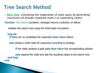
19. function Tree-Search (problem) returns a solution, or failure
List_toExplore ← Insert(Make-Node (Initial_State[problem]))
loop do
if List_toExplore is empty then return failure
else node ← Remove(List_toExplore)
if Goal-Test(problem, State(node)) then return node
else List_toExplore ←InsertAll(Expand(node, problem), List_toExplore)
EndLoop

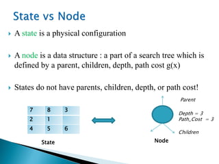
20. function Expand( node, problem) returns a set of nodes
successors← 
for each (action, result) in Successor-Function (problem, State[node]) do
N← new Node
Parent [N] ← node;
Action[N]←action;
State[N]←result
Path_Cost[N]←Path-Cost[node] + Step_Cost(State[node], (action, result))
Depth[N]←Depth[node] + 1
add N to successors
return successors

21.  A strategy : defines the choice order of node expansion
 Two types of exploration strategies
◦ Uninformed Explorations: Blind Search Methods
◦ Informed Explorations: Heuristic Search Methods

22.  Evaluation Criteria: search methods are evaluated
according to the following criteria:
Completeness: Does the method always find a solution if
one exists?
Complexity in time: How long does it take to find the
solution? ⇨ Number of expanded nodes
Complexity in space: Which memory size does it take to
perform the search? ⇨ Maximum Number of nodes in
memory
Optimality: Does the method always find the best
solution with the least cost?

23.  Time and space complexities are measured in terms of:
◦ b = maximum branching factor of the search tree
◦ d = depth level of the best (or least cost) solution
node
◦ m = maximum depth level of the search space (state
space or search tree) → can be infinite

24.  Uninformed strategies use only the information
available in the problem definition
 Breadth-first search
 Depth-first search
 Depth-limited search
 Iterative deepening search

25.  Basic Idea: Priority to expand the least recently
(shallowest) generated nodes
 Implementation : List_toExplore is implemented as
a FIFO queue : new successor go at end

26. List_toExplore : A List_toExplore : B C
List_toExplore : C D E List_toExplore : D E F G
Expanding Order : A B C D E F G

27.  Complete ??
 Time ??
 Space ??
 Optimal ??

28.  Complete ? Yes (if b is finite)
 Time ?? 1 + b + b2 + b3 + … + bd = O(bd) (exp.
In d)
 Space ?? O(bd) (each expanded node must be
kept in memory)
 Optimal ?? Yes (if cost = 1 per step); not optimal
in general
⇨Space is the big problem;

29.  Apply the Breadth First strategy to solve the
following problem
Initial Configuration Final Configuration
1 3
2
6
5
8
4
7
1 3
2
4
8
6 5
7

30. 30
1 2
8 6
3
7 5 4
1 2
3
8 6
7 5 4
1 2
4
8 6
3
7 5
1 2
6
8
3
7 5 4
1
3
8 6
2
7 5 4
1 2
4
8 6
2
7 5
1
6
8 2
3
7 5 4
1 2
6
8 5
2
7 4
1 2
6
8
2
7 5 4
1 6
3
8
2
7 5 4
1
3
8 6
2
7 5 4
1 2
8 4
3
7 6 5
Initial State
(0)
Goal State
(1) (2) (3)
(4) (5) (6) (7) (8)
(11)
(10)
(9)

31.  Basic Idea : Expand the deepest unexpanded
node
 Implementation: List_toExplore is LIFO queue,
i.e., put successors at front
Warning : for infinite cycles!
• The search space must be finite and non-cyclic
⇨ Already expanded nodes must be eliminated to
avoid cycles

33. ……………..

34.  Nodes in this example are indicated according to
visit order

35.  Complete ??
 Time ??
 Space ??
 Optimal ??

36.  Complete ?? No: fails in infinite-depth spaces,
spaces with loops
Modify to avoid repeated states along path
⇒ complete in finite spaces
 Time ?? O(bm): terrible if m is much larger than d
but if solutions are shallower, may be much faster
than breadth-first
 Space ?? O(b * m), i.e., linear space!
 Optimal ?? No

37. ⇨ Modest requirement for a memory space
 For instance : if b = 10, d = 12 and the space of
100 octets/node
◦ Depth Search requires 12 Kbyte
◦ Breadth Search requires 111 Tera-byte
* 1010 !!!

38.  Basic Idea : it corresponds to a depth-first search
with a depth limit l ,
⇨ i.e., nodes at depth l have no successors

39.  Recursive Implementation

40.  Complete ??
 Time ??
 Space ??
 Optimal ??

41.  Complete ?? Yes if L ≥ d
 Time ?? O(bL)
 Space ?? O(b * L)
 Optimal ?? No

42.  Apply the Depth Limited Search strategy to the
solve the following problem with L =3
Initial Configuration Final Configuration
1 3
2
6
5
8
4
7
1 3
2
4
8
6 5
7

43. 1 2
8 6
3
7 5 4
Initial State
(0)
(3)
1 2
3
8 6
7 5 4
1 2
4
8 6
3
7 5
1
3
8 6
2
7 5 4
1 2
4
8 6
2
7 5
1 6
3
8
2
7 5 4
1
3
8 6
2
7 5 4
1 2
8 4
3
7 6 5
Goal State
(1) (5)
(2)
(6)
(7)
(4)

44.  Basic Idea :
The problem of Depth Limited Search is : How to define
the good value of L ?
Solution : Iterative Deepening : trying every value of L
from 0 with iterative increment
 Combine avantages of Breadth First Search and
Depth First Search
◦ optimal and complete as the Breadth First Search
◦ Economic in memory space as the Depth First Search

45.  This strategy is convenient for problems with
◦ Great search space
◦ Deepth of the solution is unknown

46.  Implementation

47. Visit Order :

48.  Complete ??
 Time ??
 Space ??
 Optimal ??

49.  Complete ?? Yes
 Time ?? (d+1)b0 + db1 + (d-1)b2 + … + bd =
O(bd)
 Space ?? O(b * d)
 Optimal ?? Yes if cost = 1 per step

50. ⇨ Uninformed methods have practical limits in
terms of time and space to be applied for a wide
category of problems
 Informed or guided methods achieve better
performances in terms of :
◦ Space and/or
◦ Time
⇨The search is guided by using a heuristic

51.  Basic Idea: use an evaluation function for each
node
◦ To estimate its promising level (or desirability)
◦ To Expand most promising unexpanded node
 Implementation: List_toExplore is a queue sorted
in decreasing order of desirability
 Special cases:
◦ greedy search
◦ A∗ search

52.  Use of a criterion to reorder any nodes to be
explored
⇨ Heuristic
 A certain measure must be established to evaluate
the "promise" of a node.
⇨ Evaluation Function f

53.  The search is guided by the the best node
according to the evaluation function
 Centered on the node with the best
chance of reaching the goal

54.  A heuristic function h is integrated in the
evaluation function f
 h(u) : heuristic that estimates the cost of moving
from one state u to the final state.
 h(n) = 0 if n is a goal state.
 This function defines an order in the exploration
process

55.  Expand the states that seem closest to a goal
state, in order to achieve a solution more
quickly.
 In this case, f(n) = h(n)

56.  Assume the following configurations
Initial Configuration
Initial State
Final Configuration
Final State
1 3
2
6
5
8
4
7
1 3
2
4
8
6 5
7

57.  f(n)=h(n)
h ???
 h: number of misplaced tokens

58. 1 2
8 6
3
7 5 4
1 2
3
8 6
7 5 4
1 2
4
8 6
3
7 5
1 2
6
8
3
7 5 4
f(n)= h(n) = 3
f(n)= h(n) =4
(2) (3)
1 2
4
8 6
2
7 5
1 2
8 4
3
7 6 5
Goal State
Initial State
f(n)= h(n) =2 f(n)= h(n) =3
f(n)= h(n) =1
f(n)= h(n) =0

59.  Find the shortest path from the initial state to
the final goal.
 In this case, f(n) = h(n) + g(n)

60. I
B
n
f*(n)
g*(n)
h*(n)
f*(n) = g*(n) + h*(n)
Initial
State
Goal
State
Node n
⇨ f*(n) represents the ideal cost (best cost) of the path crossing a
node n to reach the goal

61.  g*(n): the cost of the best path already
crossed from the initial state to the state n
 The choice of g depends on the studied field
 Example : Puzzle
g(n) : the number of moved tokens
→ the length of path from the root to n

62.  By using A* Algo. f(n)=g(n) +h(n)
with :
◦ g : number of moved tokens de jetons déplacés
◦ h: number of misplaced tokens
Initial Configuration
Initial State
Final Configuration
Final State
1 3
2
6
5
8
4
7
1 3
2
4
8
6 5
7

63. 1 2
8 6
3
7 5 4
1 2
3
8 6
7 5 4
1 2
4
8 6
3
7 5
1 2
6
8
3
7 5 4
f(n)=(0+3)
(1+4) (1+2) (1+3)
1 2
4
8 6
2
7 5
1 2
8 4
3
7 6 5
Goal State
(2+1)
(3+0)
Initial State

64. 64
Initial Configuration Final Configuration
2 3
8
6
5
1 4
7
1 3
2
4
8
6 5
7
Path ???

65. 65
puzzle with A* Algorithm
A, ..., N: states
m = misplaced tokens
d = depth or number
of moved tokens
f(x) = m(x) + d(x)
1
2 3
4
5
6
7
8
1
2 3
4
5
6
7
8
1
2 3
4
5
6
7
8
1
2 3
4
5
6
7
8
d(x)
= 0
d(x)
= 1
d(x)
= 2
d(x)
= 3
m(B)
= 5
m(A)
= 4
m(C)
= 3
m(D)
= 5
1
2 3
4
5
6
7
8 1
2 3
4
5
6
7
8
1
2 3
4
5
6
7
8
m(E)
= 3
m(F)
= 3
m(G)
= 4
1
2 3
4
5
6
7
8
m(J)
= 2
1
2 3
4
5
6
7
8
m(K)
= 4
m(H)
= 3
m(I)
= 4
1
2 3
4
5
6
7
8
1
2
3
4
5
6
7
8
d(x)
= 4
1 2 3
4
5
6
7
8
m(L)
= 1
d(x)
= 5
1 2 3
4
5
6
7
8
m(M)
= 0
1 2 3
4
5
6
7 8
m(N)
= 2

66. 66
puzzle with A* Algorithm
A, ..., N: states
m = misplaced tokens
d = depth or number
of moved tokens
f(x) = m(x) + d(x)
1
2 3
4
5
6
7
8
1
2 3
4
5
6
7
8
1
2 3
4
5
6
7
8
1
2 3
4
5
6
7
8
d(x)
= 0
d(x)
= 1
d(x)
= 2
d(x)
= 3
m(B)
= 5
m(A)
= 4
m(C)
= 3
m(D)
= 5
1
2 3
4
5
6
7
8 1
2 3
4
5
6
7
8
1
2 3
4
5
6
7
8
m(E)
= 3
m(F)
= 3
m(G)
= 4
1
2 3
4
5
6
7
8
m(J)
= 2
1
2 3
4
5
6
7
8
m(K)
= 4
m(H)
= 3
m(I)
= 4
1
2 3
4
5
6
7
8
1
2
3
4
5
6
7
8
d(x)
= 4
1 2 3
4
5
6
7
8
m(L)
= 1
d(x)
= 5
1 2 3
4
5
6
7
8
m(M)
= 0
1 2 3
4
5
6
7 8
m(N)
= 2

67. 67
puzzle with A* Algorithm
A, ..., N: states
m = misplaced tokens
d = depth or number
of moved tokens
f(x) = m(x) + d(x)
1
2 3
4
5
6
7
8
1
2 3
4
5
6
7
8
1
2 3
4
5
6
7
8
1
2 3
4
5
6
7
8
d(x)
= 0
d(x)
= 1
d(x)
= 2
d(x)
= 3
m(B)
= 5
m(A)
= 4
m(C)
= 3
m(D)
= 5
1
2 3
4
5
6
7
8 1
2 3
4
5
6
7
8
1
2 3
4
5
6
7
8
m(E)
= 3
m(F)
= 3
m(G)
= 4
1
2 3
4
5
6
7
8
m(J)
= 2
1
2 3
4
5
6
7
8
m(K)
= 4
m(H)
= 3
m(I)
= 4
1
2 3
4
5
6
7
8
1
2
3
4
5
6
7
8
d(x)
= 4
1 2 3
4
5
6
7
8
m(L)
= 1
d(x)
= 5
1 2 3
4
5
6
7
8
m(M)
= 0
1 2 3
4
5
6
7 8
m(N)
= 2

68. 68
puzzle with A* Algorithm
A, ..., N: states
m = misplaced tokens
d = depth or number
of moved tokens
f(x) = m(x) + d(x)
1
2 3
4
5
6
7
8
1
2 3
4
5
6
7
8
1
2 3
4
5
6
7
8
1
2 3
4
5
6
7
8
d(x)
= 0
d(x)
= 1
d(x)
= 2
d(x)
= 3
m(B)
= 5
m(A)
= 4
m(C)
= 3
m(D)
= 5
1
2 3
4
5
6
7
8 1
2 3
4
5
6
7
8
1
2 3
4
5
6
7
8
m(E)
= 3
m(F)
= 3
m(G)
= 4
1
2 3
4
5
6
7
8
m(J)
= 2
1
2 3
4
5
6
7
8
m(K)
= 4
m(H)
= 3
m(I)
= 4
1
2 3
4
5
6
7
8
1
2
3
4
5
6
7
8
d(x)
= 4
1 2 3
4
5
6
7
8
m(L)
= 1
d(x)
= 5
1 2 3
4
5
6
7
8
m(M)
= 0
1 2 3
4
5
6
7 8
m(N)
= 2

69. 69
puzzle with A* Algorithm
A, ..., N: states
m = misplaced tokens
d = depth or number
of moved tokens
f(x) = m(x) + d(x)
1
2 3
4
5
6
7
8
1
2 3
4
5
6
7
8
1
2 3
4
5
6
7
8
1
2 3
4
5
6
7
8
d(x)
= 0
d(x)
= 1
d(x)
= 2
d(x)
= 3
m(B)
= 5
m(A)
= 4
m(C)
= 3
m(D)
= 5
1
2 3
4
5
6
7
8 1
2 3
4
5
6
7
8
1
2 3
4
5
6
7
8
m(E)
= 3
m(F)
= 3
m(G)
= 4
1
2 3
4
5
6
7
8
m(J)
= 2
1
2 3
4
5
6
7
8
m(K)
= 4
m(H)
= 3
m(I)
= 4
1
2 3
4
5
6
7
8
1
2
3
4
5
6
7
8
d(x)
= 4
1 2 3
4
5
6
7
8
m(L)
= 1
d(x)
= 5
1 2 3
4
5
6
7
8
m(M)
= 0
1 2 3
4
5
6
7 8
m(N)
= 2

70. 70
puzzle with A* Algorithm
A, ..., N: states
m = misplaced tokens
d = depth or number
of moved tokens
f(x) = m(x) + d(x)
1
2 3
4
5
6
7
8
1
2 3
4
5
6
7
8
1
2 3
4
5
6
7
8
1
2 3
4
5
6
7
8
d(x)
= 0
d(x)
= 1
d(x)
= 2
d(x)
= 3
m(B)
= 5
m(A)
= 4
m(C)
= 3
m(D)
= 5
1
2 3
4
5
6
7
8 1
2 3
4
5
6
7
8
1
2 3
4
5
6
7
8
m(E)
= 3
m(F)
= 3
m(G)
= 4
1
2 3
4
5
6
7
8
m(J)
= 2
1
2 3
4
5
6
7
8
m(K)
= 4
m(H)
= 3
m(I)
= 4
1
2 3
4
5
6
7
8
1
2
3
4
5
6
7
8
d(x)
= 4
1 2 3
4
5
6
7
8
m(L)
= 1
d(x)
= 5
1 2 3
4
5
6
7
8
m(M)
= 0
1 2 3
4
5
6
7 8
m(N)
= 2

71. 71
puzzle with A* Algorithm
A, ..., N: states
m = misplaced tokens
d = depth or number
of moved tokens
f(x) = m(x) + d(x)
1
2 3
4
5
6
7
8
1
2 3
4
5
6
7
8
1
2 3
4
5
6
7
8
1
2 3
4
5
6
7
8
d(x)
= 0
d(x)
= 1
d(x)
= 2
d(x)
= 3
m(B)
= 5
m(A)
= 4
m(C)
= 3
m(D)
= 5
1
2 3
4
5
6
7
8 1
2 3
4
5
6
7
8
1
2 3
4
5
6
7
8
m(E)
= 3
m(F)
= 3
m(G)
= 4
1
2 3
4
5
6
7
8
m(J)
= 2
1
2 3
4
5
6
7
8
m(K)
= 4
m(H)
= 3
m(I)
= 4
1
2 3
4
5
6
7
8
1
2
3
4
5
6
7
8
d(x)
= 4
1 2 3
4
5
6
7
8
m(L)
= 1
d(x)
= 5
1 2 3
4
5
6
7
8
m(M)
= 0
1 2 3
4
5
6
7 8
m(N)
= 2

72. 72
puzzle with A* Algorithm
A, ..., N: states
m = misplaced tokens
d = depth or number
of moved tokens
f(x) = m(x) + d(x)
1
2 3
4
5
6
7
8
1
2 3
4
5
6
7
8
1
2 3
4
5
6
7
8
1
2 3
4
5
6
7
8
d(x)
= 0
d(x)
= 1
d(x)
= 2
d(x)
= 3
m(B)
= 5
m(A)
= 4
m(C)
= 3
m(D)
= 5
1
2 3
4
5
6
7
8 1
2 3
4
5
6
7
8
1
2 3
4
5
6
7
8
m(E)
= 3
m(F)
= 3
m(G)
= 4
1
2 3
4
5
6
7
8
m(J)
= 2
1
2 3
4
5
6
7
8
m(K)
= 4
m(H)
= 3
m(I)
= 4
1
2 3
4
5
6
7
8
1
2
3
4
5
6
7
8
d(x)
= 4
1 2 3
4
5
6
7
8
m(L)
= 1
d(x)
= 5
1 2 3
4
5
6
7
8
m(M)
= 0
1 2 3
4
5
6
7 8
m(N)
= 2

73. 73
puzzle with A* Algorithm
A, ..., N: states
m = misplaced tokens
d = depth or number
of moved tokens
f(x) = m(x) + d(x)
1
2 3
4
5
6
7
8
1
2 3
4
5
6
7
8
1
2 3
4
5
6
7
8
1
2 3
4
5
6
7
8
d(x)
= 0
d(x)
= 1
d(x)
= 2
d(x)
= 3
m(B)
= 5
m(A)
= 4
m(C)
= 3
m(D)
= 5
1
2 3
4
5
6
7
8 1
2 3
4
5
6
7
8
1
2 3
4
5
6
7
8
m(E)
= 3
m(F)
= 3
m(G)
= 4
1
2 3
4
5
6
7
8
m(J)
= 2
1
2 3
4
5
6
7
8
m(K)
= 4
m(H)
= 3
m(I)
= 4
1
2 3
4
5
6
7
8
1
2
3
4
5
6
7
8
d(x)
= 4
1 2 3
4
5
6
7
8
m(L)
= 1
d(x)
= 5
1 2 3
4
5
6
7
8
m(M)
= 0
1 2 3
4
5
6
7 8
m(N)
= 2

74. 74
puzzle with A* Algorithm
A, ..., N: states
m = misplaced tokens
d = depth or number
of moved tokens
f(x) = m(x) + d(x)
1
2 3
4
5
6
7
8
1
2 3
4
5
6
7
8
1
2 3
4
5
6
7
8
1
2 3
4
5
6
7
8
d(x)
= 0
d(x)
= 1
d(x)
= 2
d(x)
= 3
m(B)
= 5
m(A)
= 4
m(C)
= 3
m(D)
= 5
1
2 3
4
5
6
7
8 1
2 3
4
5
6
7
8
1
2 3
4
5
6
7
8
m(E)
= 3
m(F)
= 3
m(G)
= 4
1
2 3
4
5
6
7
8
m(J)
= 2
1
2 3
4
5
6
7
8
m(K)
= 4
m(H)
= 3
m(I)
= 4
1
2 3
4
5
6
7
8
1
2
3
4
5
6
7
8
d(x)
= 4
1 2 3
4
5
6
7
8
m(L)
= 1
d(x)
= 5
1 2 3
4
5
6
7
8
m(M)
= 0
1 2 3
4
5
6
7 8
m(N)
= 2

75. 75
puzzle with A* Algorithm
A, ..., N: states
m = misplaced tokens
d = depth or number
of moved tokens
f(x) = m(x) + d(x)
1
2 3
4
5
6
7
8
1
2 3
4
5
6
7
8
1
2 3
4
5
6
7
8
1
2 3
4
5
6
7
8
d(x)
= 0
d(x)
= 1
d(x)
= 2
d(x)
= 3
m(B)
= 5
m(A)
= 4
m(C)
= 3
m(D)
= 5
1
2 3
4
5
6
7
8 1
2 3
4
5
6
7
8
1
2 3
4
5
6
7
8
m(E)
= 3
m(F)
= 3
m(G)
= 4
1
2 3
4
5
6
7
8
m(J)
= 2
1
2 3
4
5
6
7
8
m(K)
= 4
m(H)
= 3
m(I)
= 4
1
2 3
4
5
6
7
8
1
2
3
4
5
6
7
8
d(x)
= 4
1 2 3
4
5
6
7
8
m(L)
= 1
d(x)
= 5
1 2 3
4
5
6
7
8
m(M)
= 0
1 2 3
4
5
6
7 8
m(N)
= 2
Final
State

76.  Assume a postman initially in the city of Arad in
Romania
 the goal is to attain Bucharest with the minimal
cost path
 The shortest path ???
 Greedy Search ?
 A* Algorithm ?

77. Straight-line
distance to
Bucharest
Romania Step
Cost in Km