bài toán vận chuyển

1. Operations Research I
Transportation problems
Ing. Lenka Skanderová, Ph.D.

2. Factory
Goods
Warehouse
Ship
Typical example
• Introduction
• Model creation
• Initial BF solution
• Optimality test
2/60
Operations research I

3. P & T Company
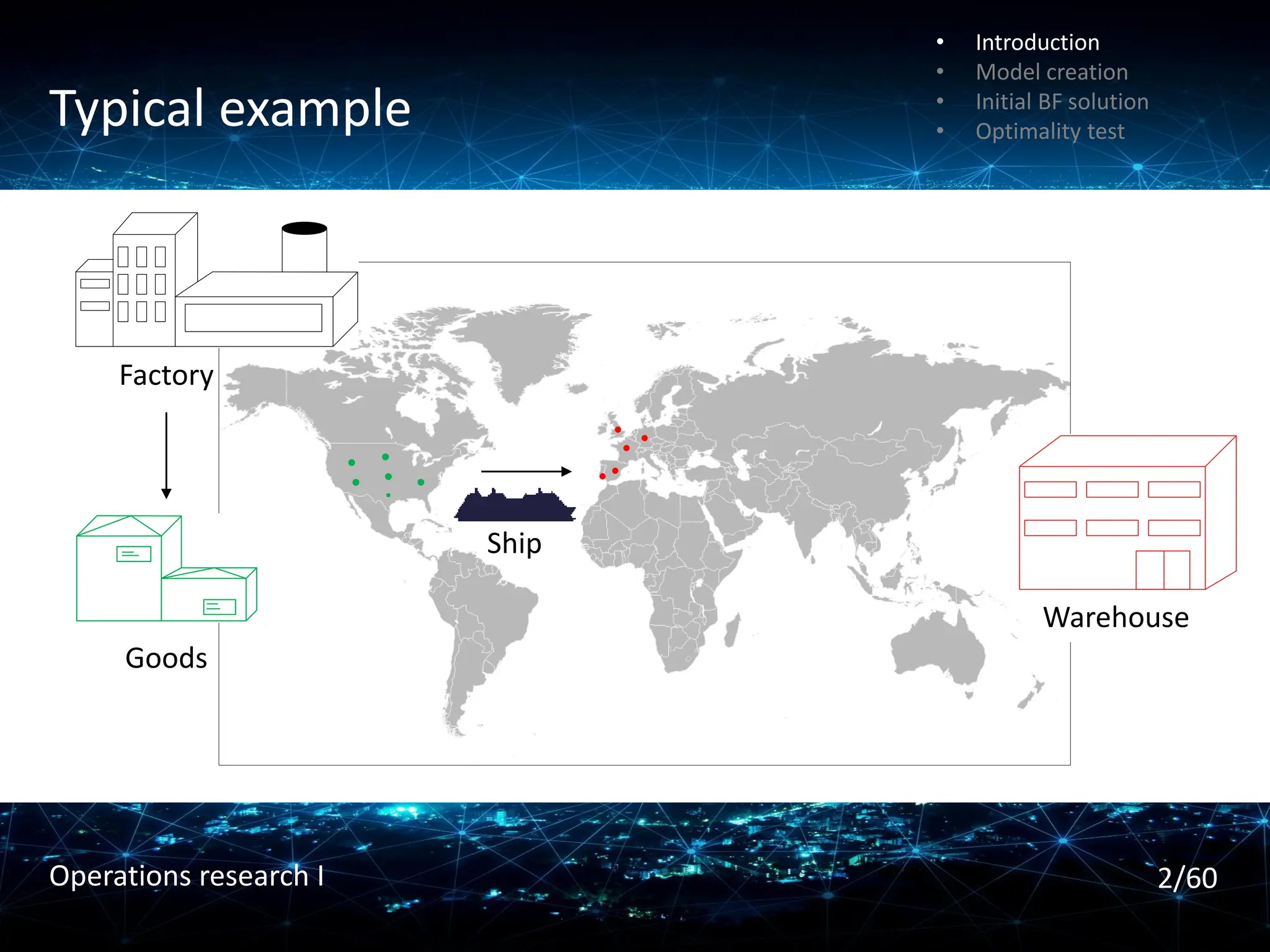
• Product: canned peas
• Canneries:
• Bellingham, Washington
• Eugene, Oregon
• Albert Lea, Minesota
• Warehouses
• Sacramento, California
• Salt Lake City, Utah
• Rapid City, South Dakota,
• Albuquerque, New Mexico
• Shipping costs are the major expense COST MINIMIZATION
• Introduction
• Model creation
• Initial BF solution
• Optimality test
3/60
Operations research I

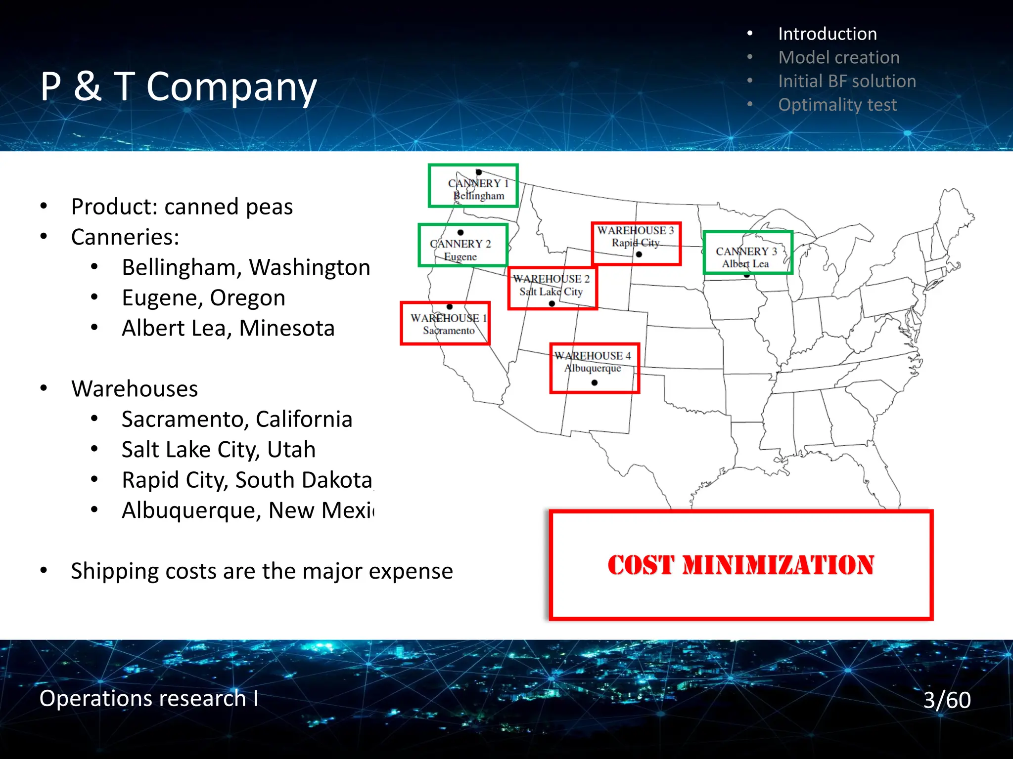
4. P & T Company
Table
Shipping Cost ($) per Truckload
Warehouse
1 2 3 4 Output
Cannery 1 464 513 654 867 75
2 352 416 690 791 125
3 995 682 388 685 100
Allocation 80 65 70 85
Constraints of warehouses
Constraints
of canneries
• Introduction
• Model creation
• Initial BF solution
• Optimality test
4/60
Operations research I

5. P & T Company
Model creation
𝑍 = 464𝑥11 + 513𝑥12 + 654𝑥13 + 867𝑥14 + 352𝑥21 + 416𝑥22 + 690𝑥23 +
791𝑥24 + 995𝑥31 + 682𝑥32 + 388𝑥33 + 685𝑥34
• Minimize
• Subject to:
𝑥11 + 𝑥12 + 𝑥13 + 𝑥14 = 75
𝑥21 + 𝑥22 + 𝑥23 + 𝑥24 = 125
𝑥31 + 𝑥32 + 𝑥33 + 𝑥34 = 100
𝑥11 + 𝑥21 + 𝑥31 = 80
𝑥12 + 𝑥22 + 𝑥32 = 65
𝑥13 + 𝑥23 + 𝑥33 = 70
𝑥14 + 𝑥24 + 𝑥34 = 85
Typical structure of constraint coefficients in the transportation problem
• Introduction
• Model creation
• Initial BF solution
• Optimality test
5/60
Operations research I

6. P & T Company
Model creation
𝑍 = 464𝑥11 + 513𝑥12 + 654𝑥13 + 867𝑥14 + 352𝑥21 + 416𝑥22 + 690𝑥23 +
791𝑥24 + 995𝑥31 + 682𝑥32 + 388𝑥33 + 685𝑥34
• Minimize
• Subject to:
𝑥11 + 𝑥12 + 𝑥13 + 𝑥14 = 75
𝑥21 + 𝑥22 + 𝑥23 + 𝑥24 = 125
𝑥31 + 𝑥32 + 𝑥33 + 𝑥34 = 100
𝑥11 + 𝑥21 + 𝑥31 = 80
𝑥12 + 𝑥22 + 𝑥32 = 65
𝑥13 + 𝑥23 + 𝑥33 = 70
𝑥14 + 𝑥24 + 𝑥34 = 85
Do not forget the nonnegative coefficients! 𝑥𝑖𝑗 ≥ 0
• Introduction
• Model creation
• Initial BF solution
• Optimality test
6/60
Operations research I

7. P & T Company
Graph representation
C1
C2
C3
W1
W2
W4
W3
[75]
[125]
[100]
[-80]
[-65]
[-70]
[-85]
• Introduction
• Model creation
• Initial BF solution
• Optimality test
7/60
Operations research I

8. Transportation problem
Assumptions
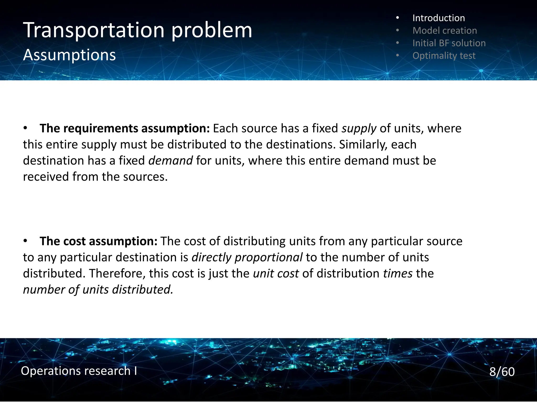
• The requirements assumption: Each source has a fixed supply of units, where
this entire supply must be distributed to the destinations. Similarly, each
destination has a fixed demand for units, where this entire demand must be
received from the sources.
• The cost assumption: The cost of distributing units from any particular source
to any particular destination is directly proportional to the number of units
distributed. Therefore, this cost is just the unit cost of distribution times the
number of units distributed.
• Introduction
• Model creation
• Initial BF solution
• Optimality test
8/60
Operations research I

9. Transportation problem
Feasible solution
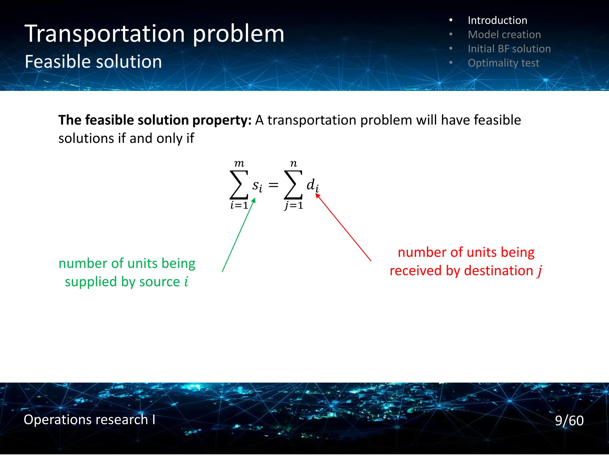
The feasible solution property: A transportation problem will have feasible
solutions if and only if
෍
𝑖=1
𝑚
𝑠𝑖 = ෍
𝑗=1
𝑛
𝑑𝑖
number of units being
supplied by source 𝑖
number of units being
received by destination 𝑗
• Introduction
• Model creation
• Initial BF solution
• Optimality test
9/60
Operations research I

10. Transportation problem
General structure
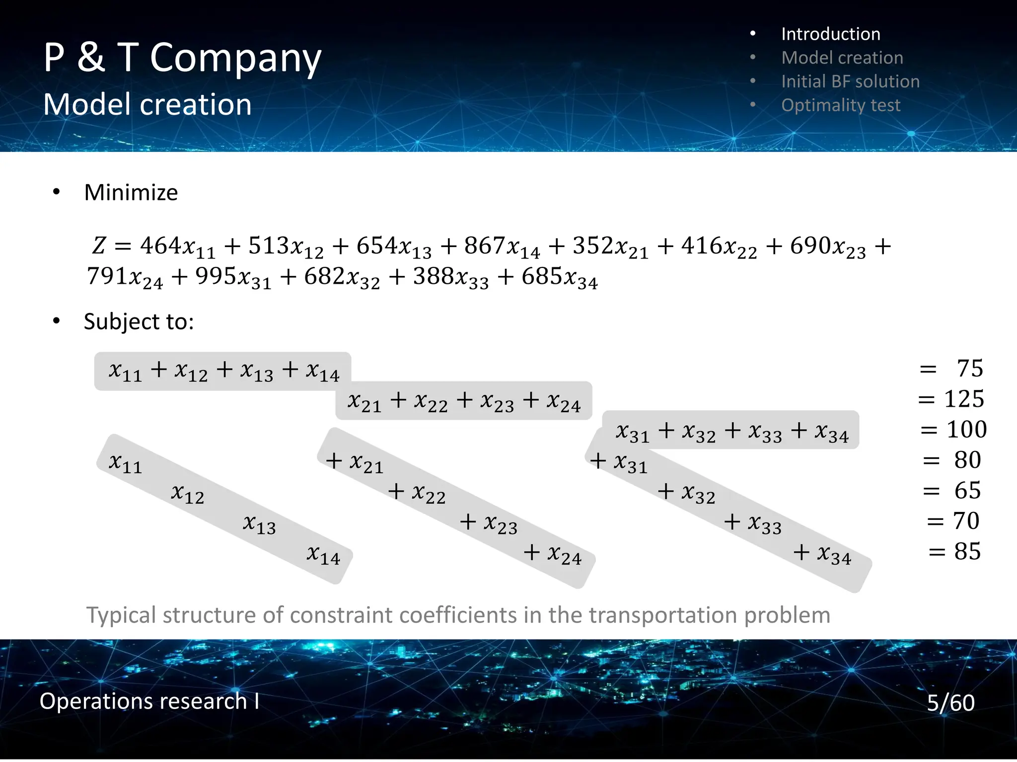
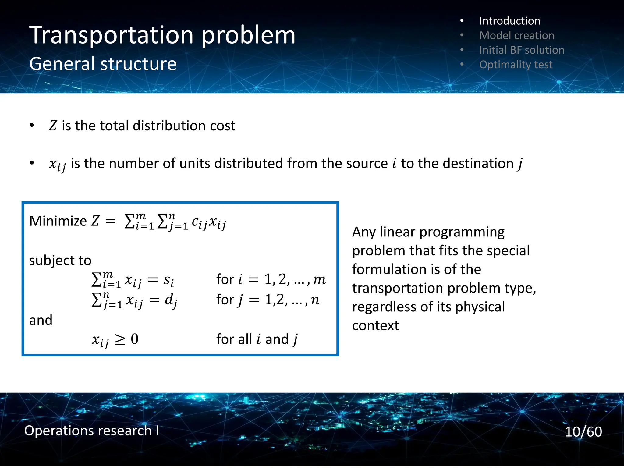
• 𝑍 is the total distribution cost
• 𝑥𝑖𝑗 is the number of units distributed from the source 𝑖 to the destination 𝑗
Minimize 𝑍 = σ𝑖=1
𝑚 σ𝑗=1
𝑛
𝑐𝑖𝑗𝑥𝑖𝑗
subject to
σ𝑖=1
𝑚
𝑥𝑖𝑗 = 𝑠𝑖 for 𝑖 = 1, 2, … , 𝑚
σ𝑗=1
𝑛
𝑥𝑖𝑗 = 𝑑𝑗 for 𝑗 = 1,2, … , 𝑛
and
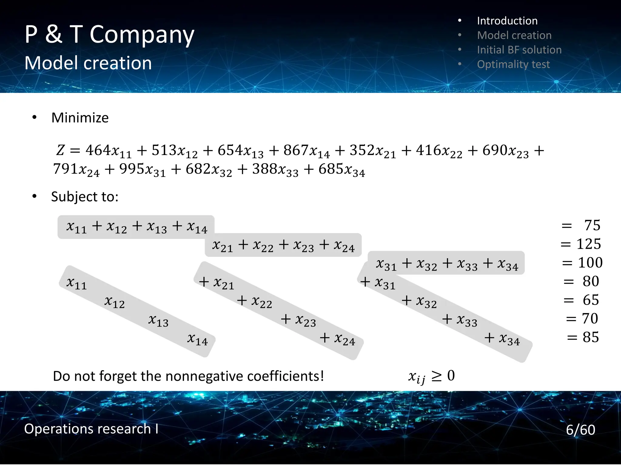
𝑥𝑖𝑗 ≥ 0 for all 𝑖 and 𝑗
Any linear programming
problem that fits the special
formulation is of the
transportation problem type,
regardless of its physical
context
• Introduction
• Model creation
• Initial BF solution
• Optimality test
10/60
Operations research I

11. Transportation problem
General structure
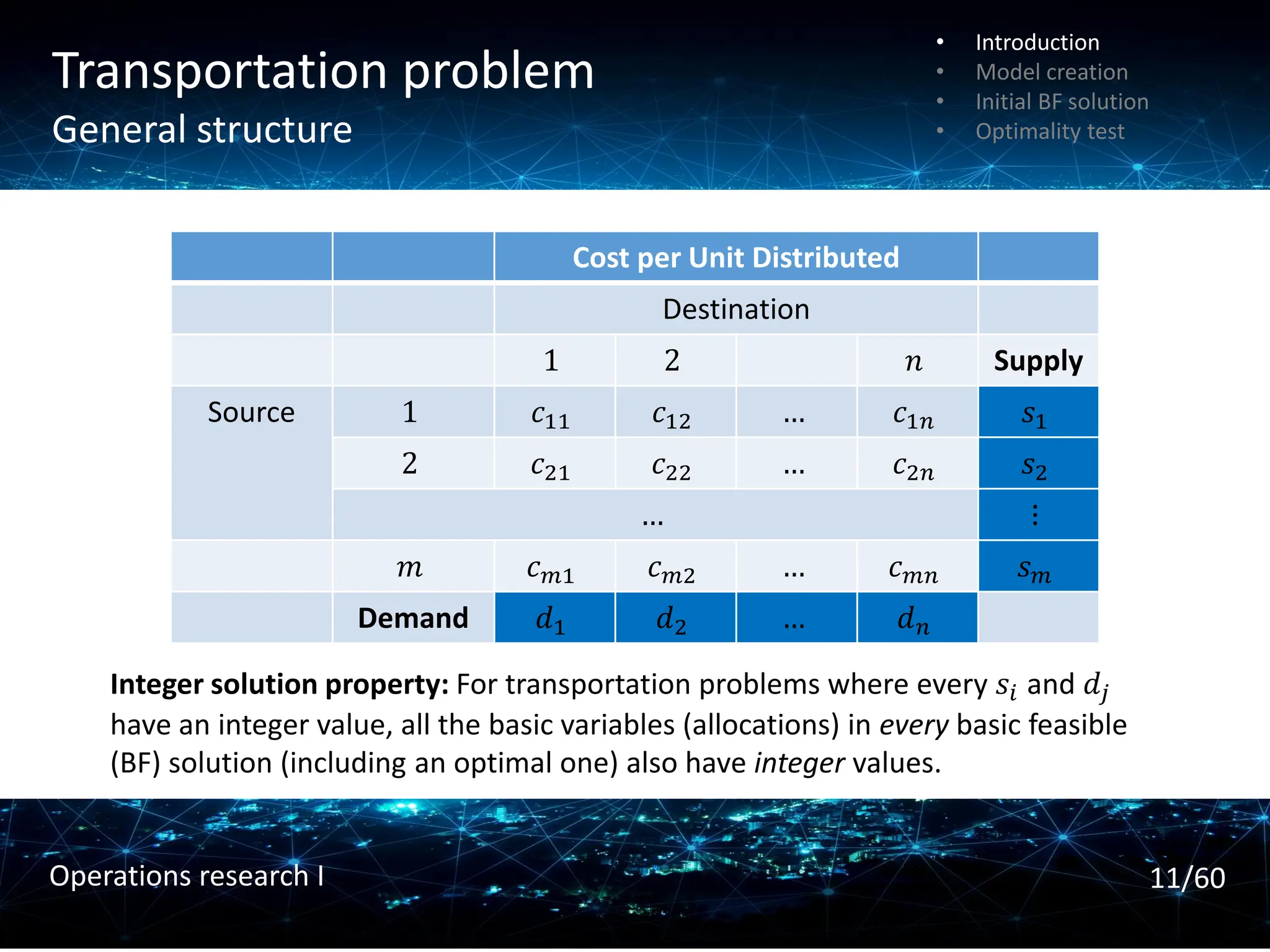
Cost per Unit Distributed
Destination
1 2 𝑛 Supply
Source 1 𝑐11 𝑐12 … 𝑐1𝑛 𝑠1
2 𝑐21 𝑐22 … 𝑐2𝑛 𝑠2
… ⋮
𝑚 𝑐𝑚1 𝑐𝑚2 … 𝑐𝑚𝑛 𝑠𝑚
Demand 𝑑1 𝑑2 … 𝑑𝑛
Integer solution property: For transportation problems where every 𝑠𝑖 and 𝑑𝑗
have an integer value, all the basic variables (allocations) in every basic feasible
(BF) solution (including an optimal one) also have integer values.
• Introduction
• Model creation
• Initial BF solution
• Optimality test
11/60
Operations research I

12. Transportation problem
Example
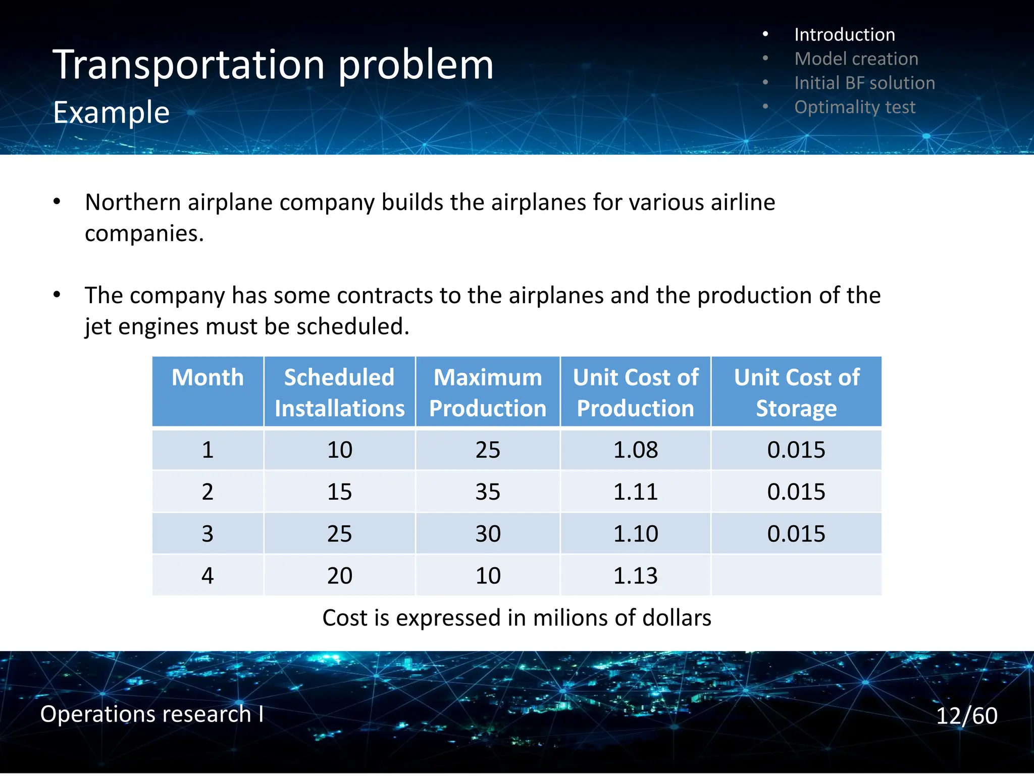
Month Scheduled
Installations
Maximum
Production
Unit Cost of
Production
Unit Cost of
Storage
1 10 25 1.08 0.015
2 15 35 1.11 0.015
3 25 30 1.10 0.015
4 20 10 1.13
Cost is expressed in milions of dollars
• Northern airplane company builds the airplanes for various airline
companies.
• The company has some contracts to the airplanes and the production of the
jet engines must be scheduled.
• Introduction
• Model creation
• Initial BF solution
• Optimality test
12/60
Operations research I

13. Transportation problem
Example
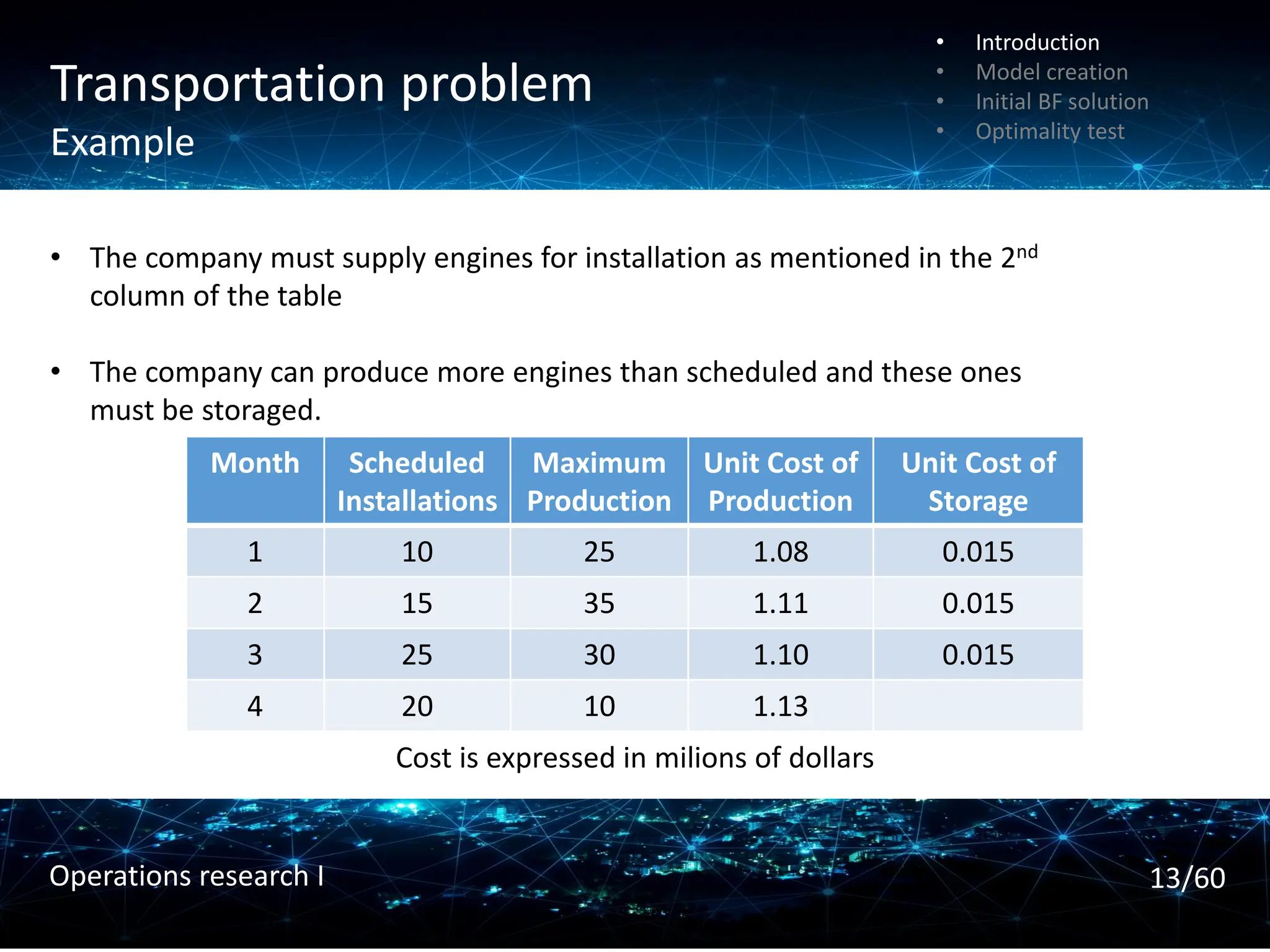
Month Scheduled
Installations
Maximum
Production
Unit Cost of
Production
Unit Cost of
Storage
1 10 25 1.08 0.015
2 15 35 1.11 0.015
3 25 30 1.10 0.015
4 20 10 1.13
Cost is expressed in milions of dollars
• The company must supply engines for installation as mentioned in the 2nd
column of the table
• The company can produce more engines than scheduled and these ones
must be storaged.
• Introduction
• Model creation
• Initial BF solution
• Optimality test
13/60
Operations research I

14. Transportation problem
Supply and demand
Month Scheduled
Installations
Maximum
Production
Unit Cost of
Production
Unit Cost of
Storage
1 10 25 1.08 0.015
2 15 35 1.11 0.015
3 25 30 1.10 0.015
4 20 10 1.13
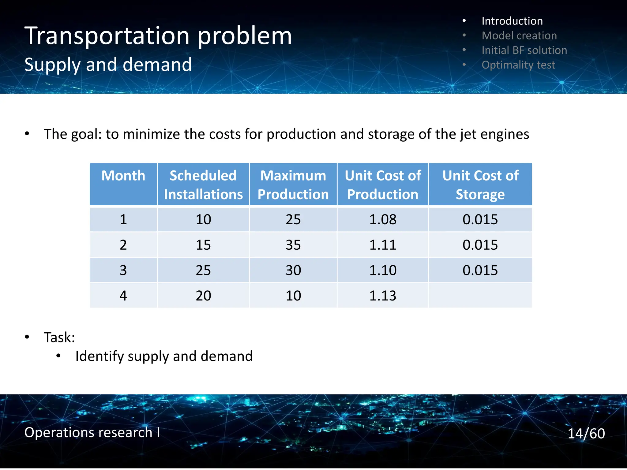
• The goal: to minimize the costs for production and storage of the jet engines
• Task:
• Identify supply and demand
• Introduction
• Model creation
• Initial BF solution
• Optimality test
14/60
Operations research I

15. Transportation problem
Supply and demand
Month Scheduled
Installations
Maximum
Production
Unit Cost of
Production
Unit Cost of
Storage
1 10 25 1.08 0.015
2 15 35 1.11 0.015
3 25 30 1.10 0.015
4 20 10 1.13
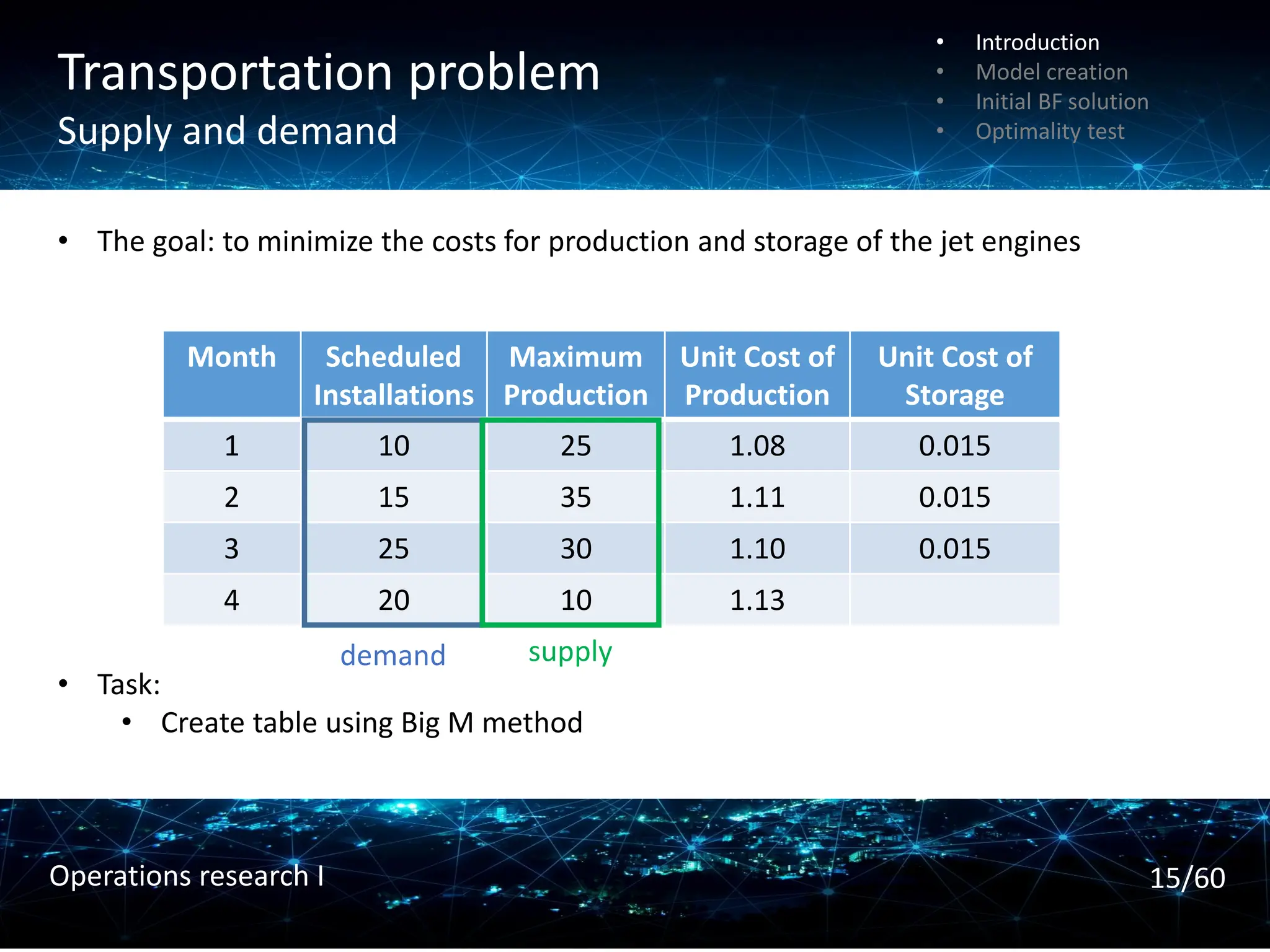
• The goal: to minimize the costs for production and storage of the jet engines
supply
demand
• Task:
• Create table using Big M method
• Introduction
• Model creation
• Initial BF solution
• Optimality test
15/60
Operations research I

16. Transportation problem
Supply and demand
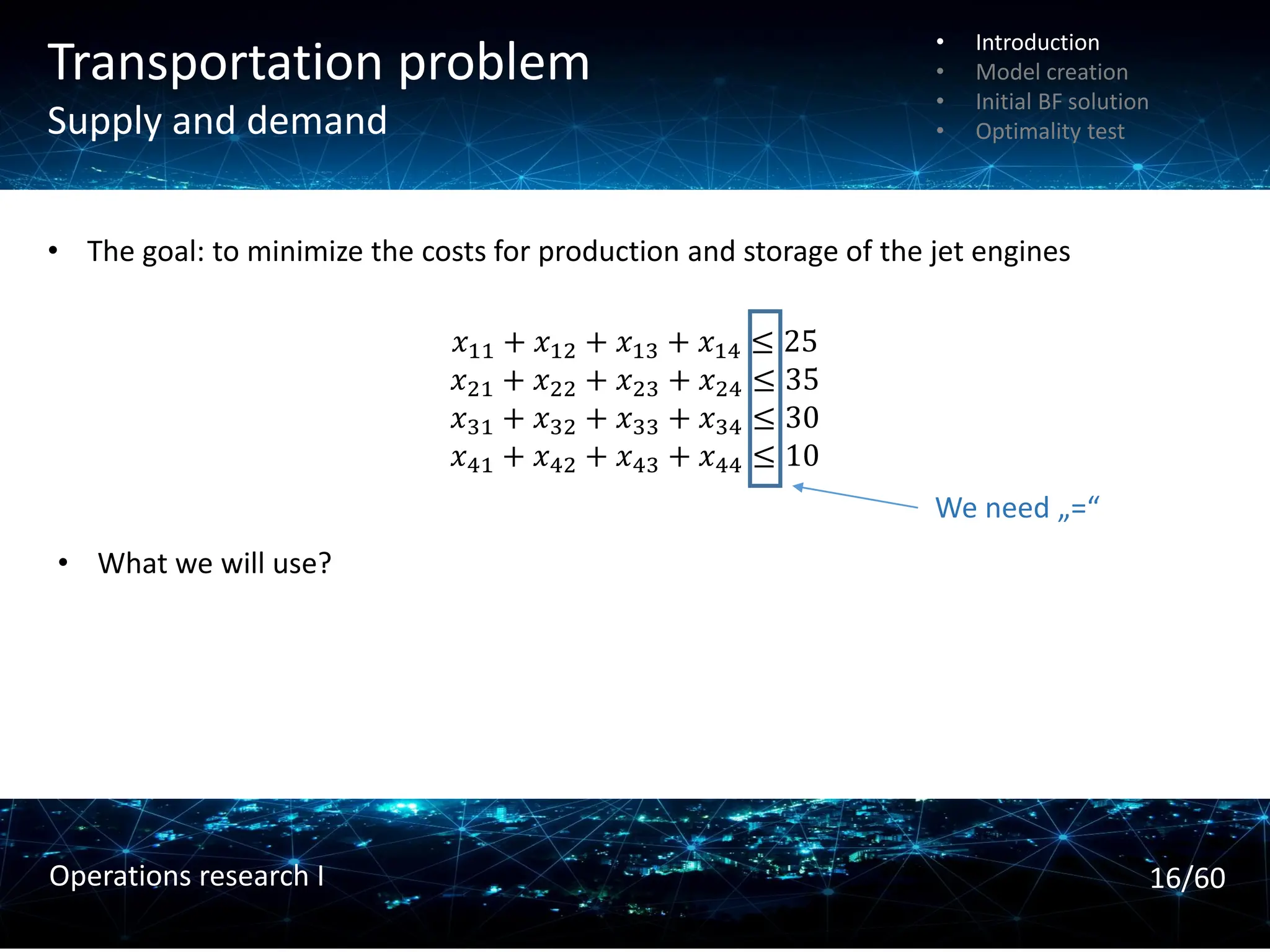
• The goal: to minimize the costs for production and storage of the jet engines
• What we will use?
𝑥11 + 𝑥12 + 𝑥13 + 𝑥14 ≤ 25
𝑥21 + 𝑥22 + 𝑥23 + 𝑥24 ≤ 35
𝑥31 + 𝑥32 + 𝑥33 + 𝑥34 ≤ 30
𝑥41 + 𝑥42 + 𝑥43 + 𝑥44 ≤ 10
We need „=“
• Introduction
• Model creation
• Initial BF solution
• Optimality test
16/60
Operations research I

17. Transportation problem
Slack variable
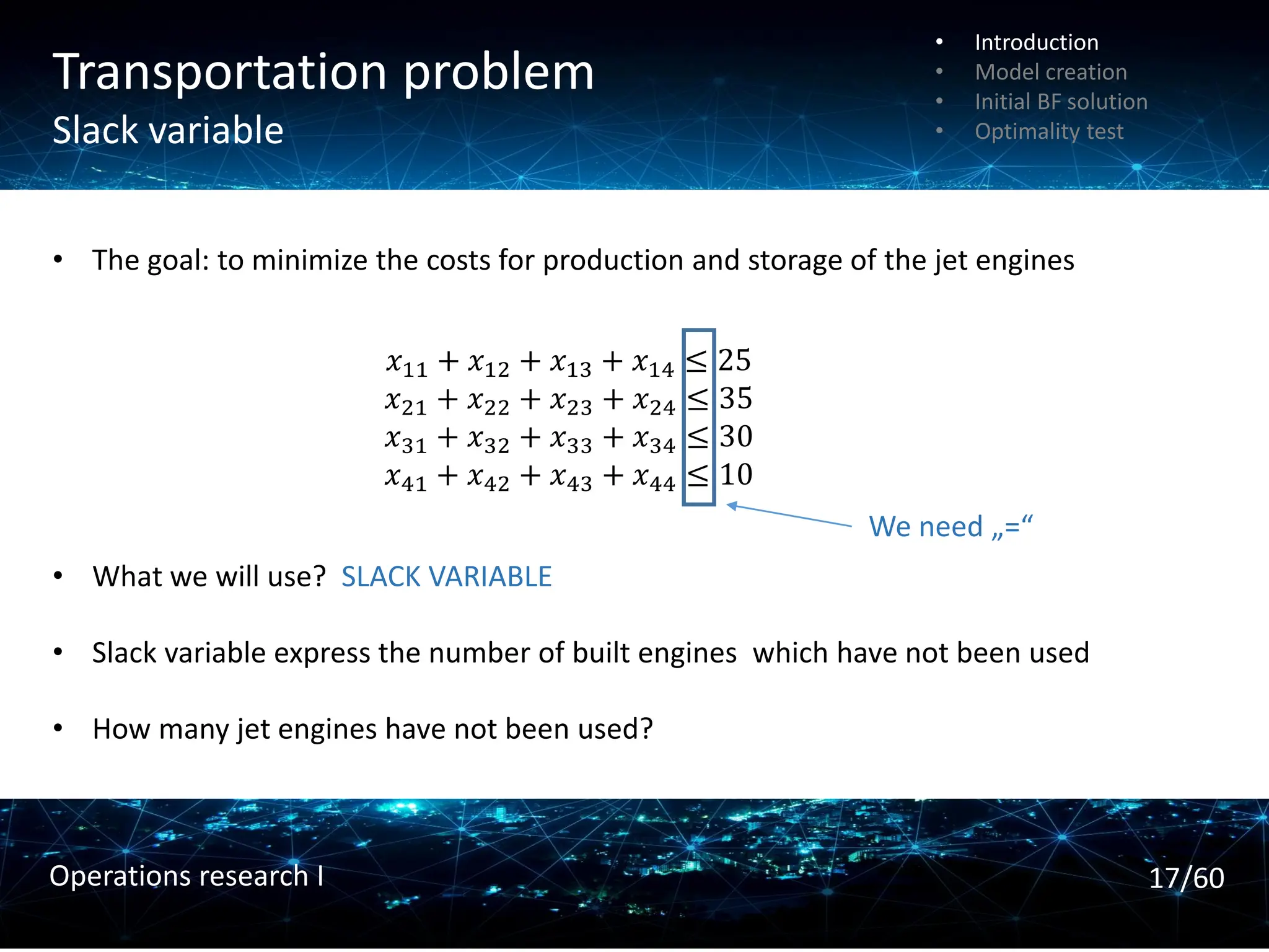
• The goal: to minimize the costs for production and storage of the jet engines
• What we will use? SLACK VARIABLE
• Slack variable express the number of built engines which have not been used
• How many jet engines have not been used?
𝑥11 + 𝑥12 + 𝑥13 + 𝑥14 ≤ 25
𝑥21 + 𝑥22 + 𝑥23 + 𝑥24 ≤ 35
𝑥31 + 𝑥32 + 𝑥33 + 𝑥34 ≤ 30
𝑥41 + 𝑥42 + 𝑥43 + 𝑥44 ≤ 10
We need „=“
• Introduction
• Model creation
• Initial BF solution
• Optimality test
17/60
Operations research I

18. Transportation problem
Slack variable
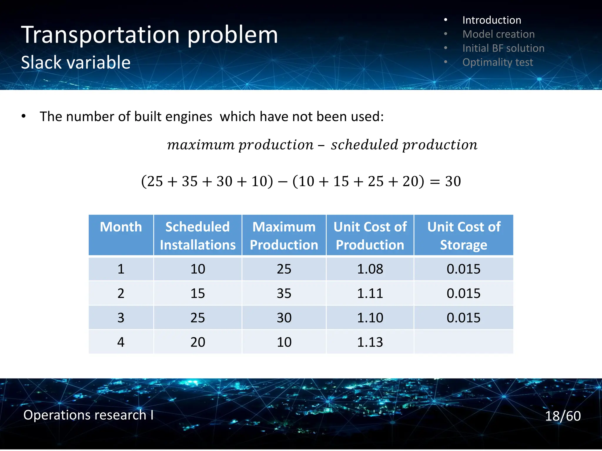
• The number of built engines which have not been used:
𝑚𝑎𝑥𝑖𝑚𝑢𝑚 𝑝𝑟𝑜𝑑𝑢𝑐𝑡𝑖𝑜𝑛 – 𝑠𝑐ℎ𝑒𝑑𝑢𝑙𝑒𝑑 𝑝𝑟𝑜𝑑𝑢𝑐𝑡𝑖𝑜𝑛
Month Scheduled
Installations
Maximum
Production
Unit Cost of
Production
Unit Cost of
Storage
1 10 25 1.08 0.015
2 15 35 1.11 0.015
3 25 30 1.10 0.015
4 20 10 1.13
25 + 35 + 30 + 10 − 10 + 15 + 25 + 20 = 30
• Introduction
• Model creation
• Initial BF solution
• Optimality test
18/60
Operations research I

19. Transportation problem
Table
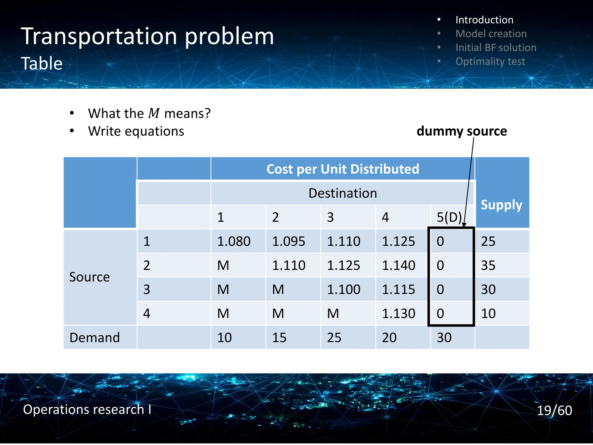
Cost per Unit Distributed
Supply
Destination
1 2 3 4 5(D)
Source
1 1.080 1.095 1.110 1.125 0 25
2 M 1.110 1.125 1.140 0 35
3 M M 1.100 1.115 0 30
4 M M M 1.130 0 10
Demand 10 15 25 20 30
• What the 𝑀 means?
• Write equations dummy source
• Introduction
• Model creation
• Initial BF solution
• Optimality test
19/60
Operations research I

20. Trensportation and assignment problems
Streamlined simplex method
Operations research I

21. Example
Water for cities
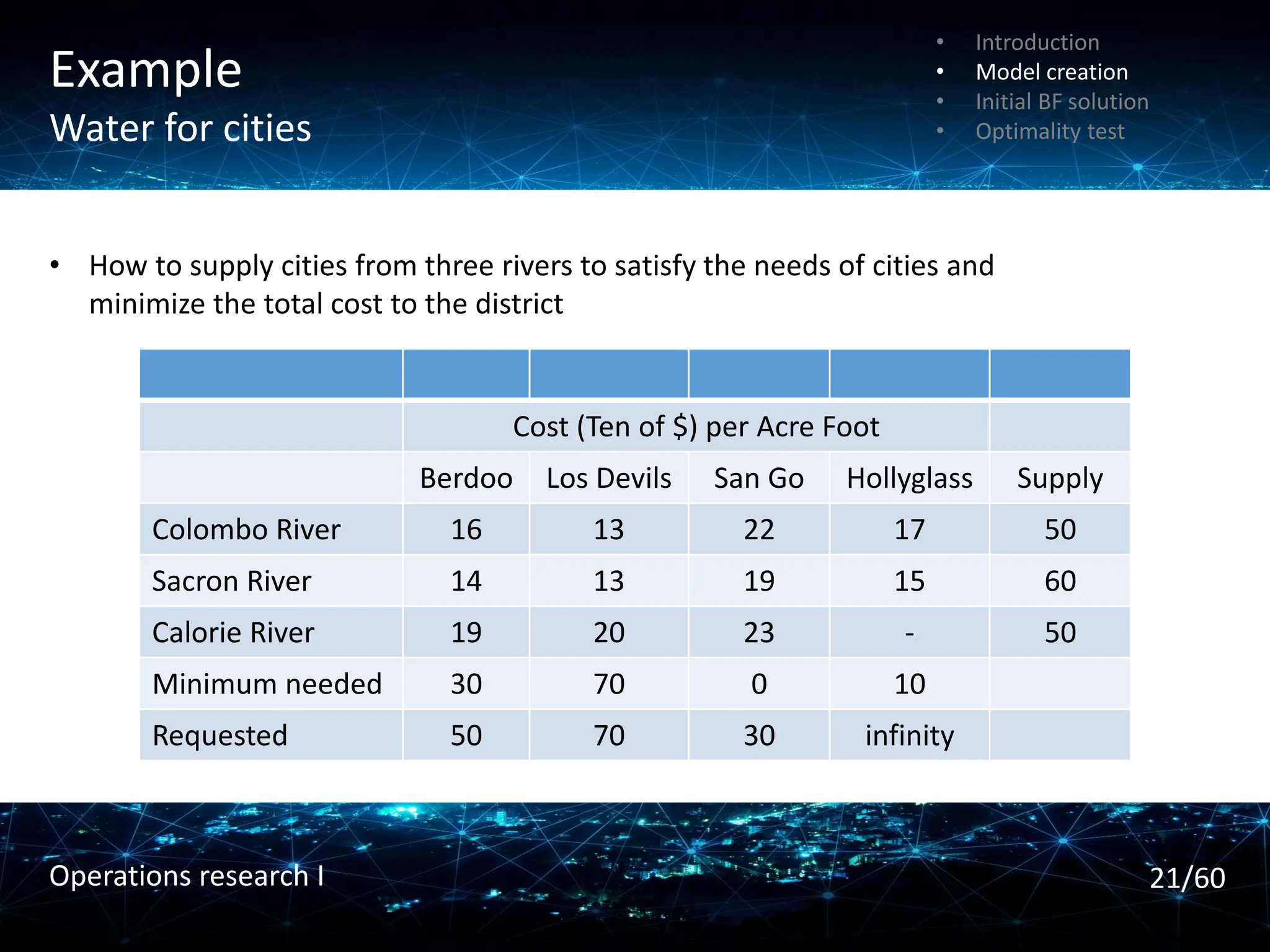
Cost (Ten of $) per Acre Foot
Berdoo Los Devils San Go Hollyglass Supply
Colombo River 16 13 22 17 50
Sacron River 14 13 19 15 60
Calorie River 19 20 23 - 50
Minimum needed 30 70 0 10
Requested 50 70 30 infinity
• How to supply cities from three rivers to satisfy the needs of cities and
minimize the total cost to the district
• Introduction
• Model creation
• Initial BF solution
• Optimality test
21/60
Operations research I

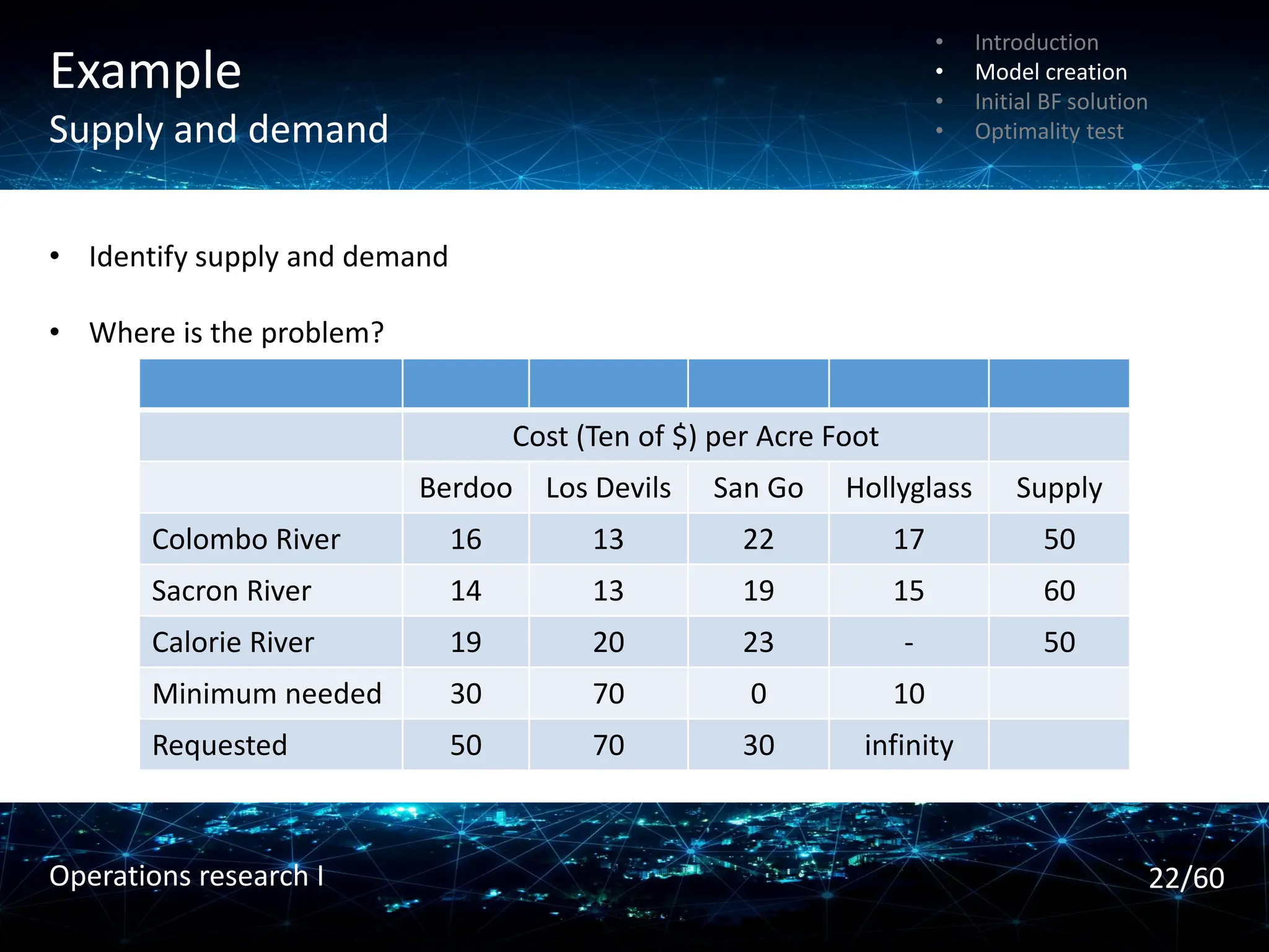
22. Example
Supply and demand
Cost (Ten of $) per Acre Foot
Berdoo Los Devils San Go Hollyglass Supply
Colombo River 16 13 22 17 50
Sacron River 14 13 19 15 60
Calorie River 19 20 23 - 50
Minimum needed 30 70 0 10
Requested 50 70 30 infinity
• Identify supply and demand
• Where is the problem?
• Introduction
• Model creation
• Initial BF solution
• Optimality test
22/60
Operations research I

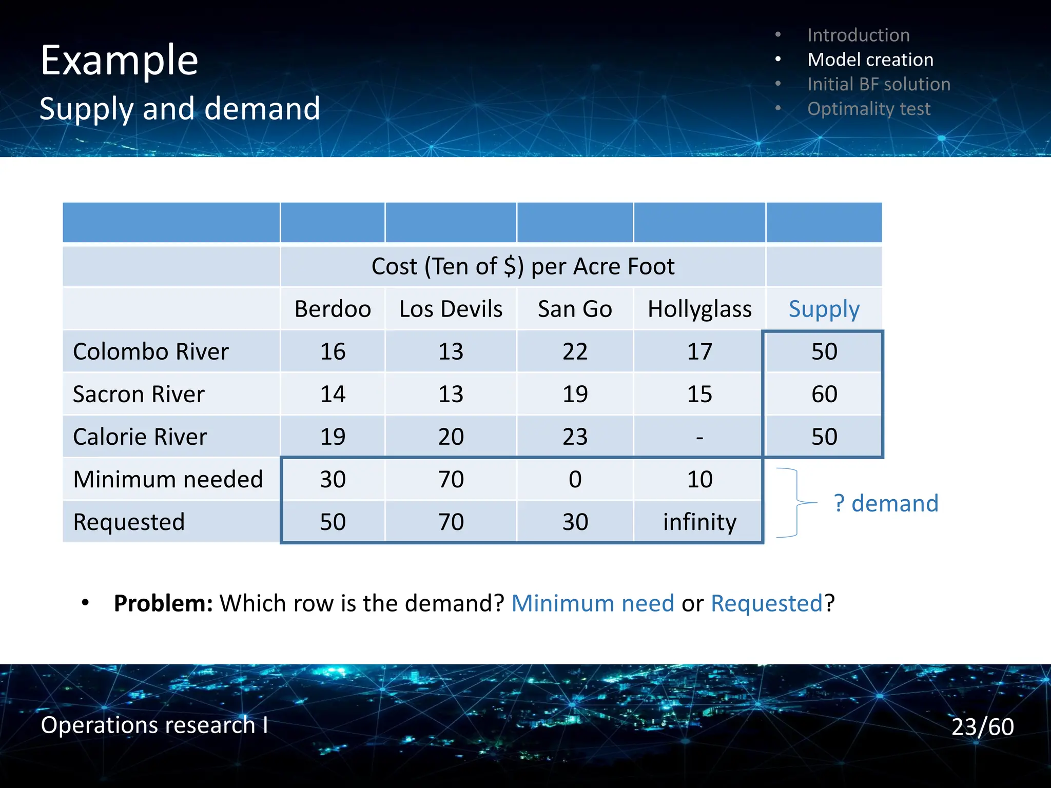
23. Example
Supply and demand
Cost (Ten of $) per Acre Foot
Berdoo Los Devils San Go Hollyglass Supply
Colombo River 16 13 22 17 50
Sacron River 14 13 19 15 60
Calorie River 19 20 23 - 50
Minimum needed 30 70 0 10
Requested 50 70 30 infinity
? demand
• Problem: Which row is the demand? Minimum need or Requested?
• Introduction
• Model creation
• Initial BF solution
• Optimality test
23/60
Operations research I

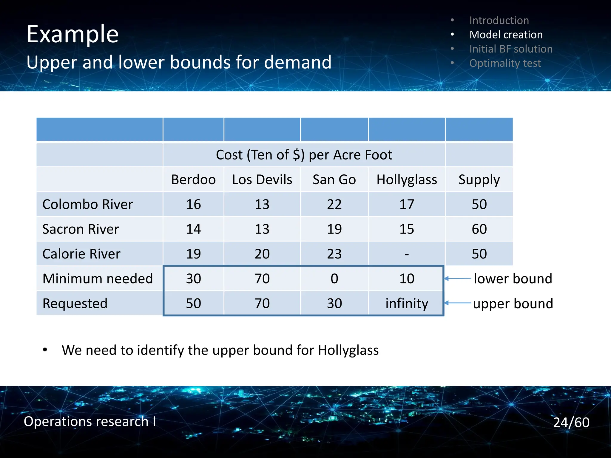
24. Example
Upper and lower bounds for demand
Cost (Ten of $) per Acre Foot
Berdoo Los Devils San Go Hollyglass Supply
Colombo River 16 13 22 17 50
Sacron River 14 13 19 15 60
Calorie River 19 20 23 - 50
Minimum needed 30 70 0 10
Requested 50 70 30 infinity
lower bound
upper bound
• We need to identify the upper bound for Hollyglass
• Introduction
• Model creation
• Initial BF solution
• Optimality test
24/60
Operations research I

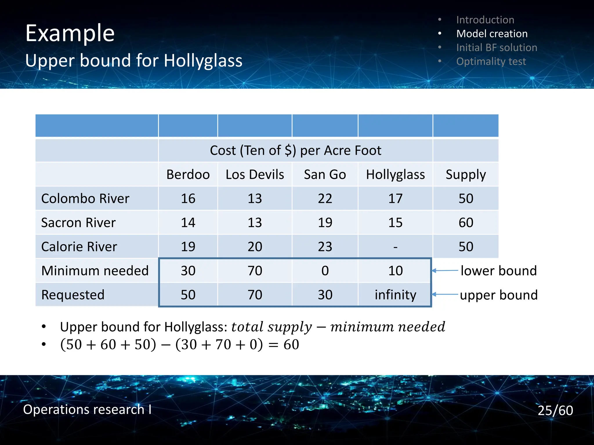
25. Example
Upper bound for Hollyglass
Cost (Ten of $) per Acre Foot
Berdoo Los Devils San Go Hollyglass Supply
Colombo River 16 13 22 17 50
Sacron River 14 13 19 15 60
Calorie River 19 20 23 - 50
Minimum needed 30 70 0 10
Requested 50 70 30 infinity
lower bound
upper bound
• Upper bound for Hollyglass: 𝑡𝑜𝑡𝑎𝑙 𝑠𝑢𝑝𝑝𝑙𝑦 − 𝑚𝑖𝑛𝑖𝑚𝑢𝑚 𝑛𝑒𝑒𝑑𝑒𝑑
• 50 + 60 + 50 − 30 + 70 + 0 = 60
• Introduction
• Model creation
• Initial BF solution
• Optimality test
25/60
Operations research I

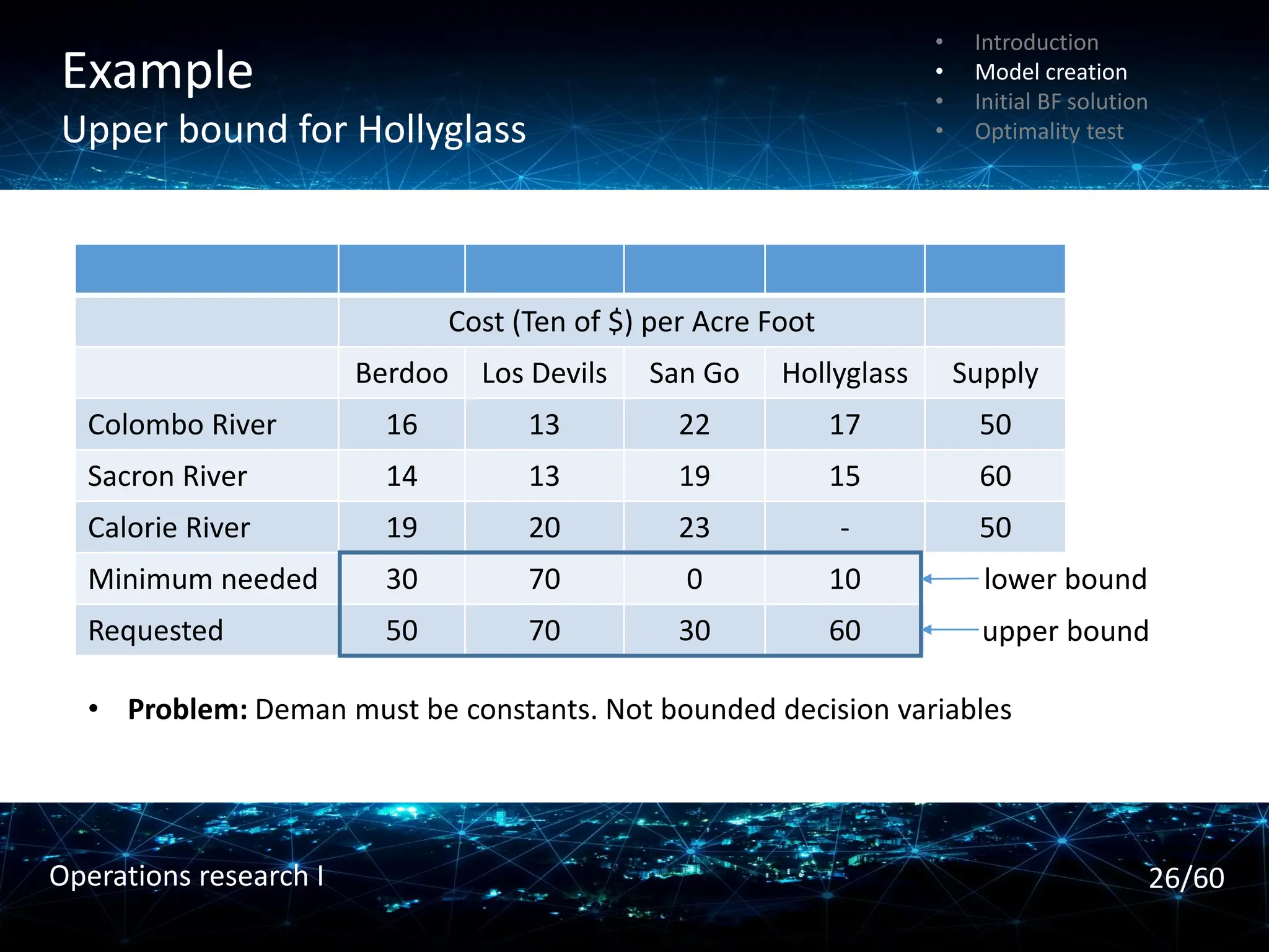
26. Example
Upper bound for Hollyglass
Cost (Ten of $) per Acre Foot
Berdoo Los Devils San Go Hollyglass Supply
Colombo River 16 13 22 17 50
Sacron River 14 13 19 15 60
Calorie River 19 20 23 - 50
Minimum needed 30 70 0 10
Requested 50 70 30 60
lower bound
upper bound
• Problem: Deman must be constants. Not bounded decision variables
• Introduction
• Model creation
• Initial BF solution
• Optimality test
26/60
Operations research I

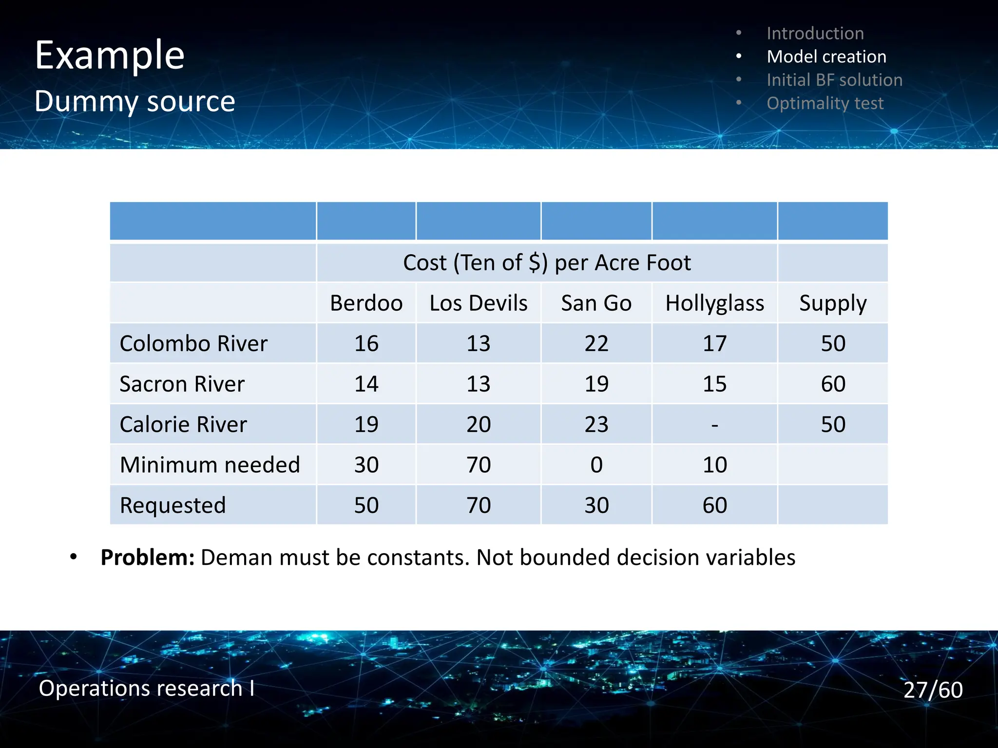
27. Example
Dummy source
Cost (Ten of $) per Acre Foot
Berdoo Los Devils San Go Hollyglass Supply
Colombo River 16 13 22 17 50
Sacron River 14 13 19 15 60
Calorie River 19 20 23 - 50
Minimum needed 30 70 0 10
Requested 50 70 30 60
• Problem: Deman must be constants. Not bounded decision variables
• Introduction
• Model creation
• Initial BF solution
• Optimality test
27/60
Operations research I

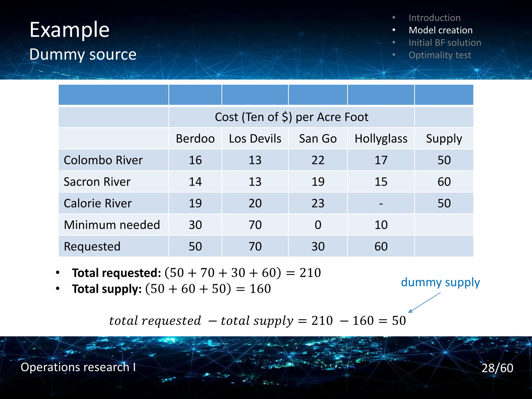
28. Example
Dummy source
Cost (Ten of $) per Acre Foot
Berdoo Los Devils San Go Hollyglass Supply
Colombo River 16 13 22 17 50
Sacron River 14 13 19 15 60
Calorie River 19 20 23 - 50
Minimum needed 30 70 0 10
Requested 50 70 30 60
• Total requested: 50 + 70 + 30 + 60 = 210
• Total supply: 50 + 60 + 50 = 160
𝑡𝑜𝑡𝑎𝑙 𝑟𝑒𝑞𝑢𝑒𝑠𝑡𝑒𝑑 − 𝑡𝑜𝑡𝑎𝑙 𝑠𝑢𝑝𝑝𝑙𝑦 = 210 − 160 = 50
dummy supply
• Introduction
• Model creation
• Initial BF solution
• Optimality test
28/60
Operations research I

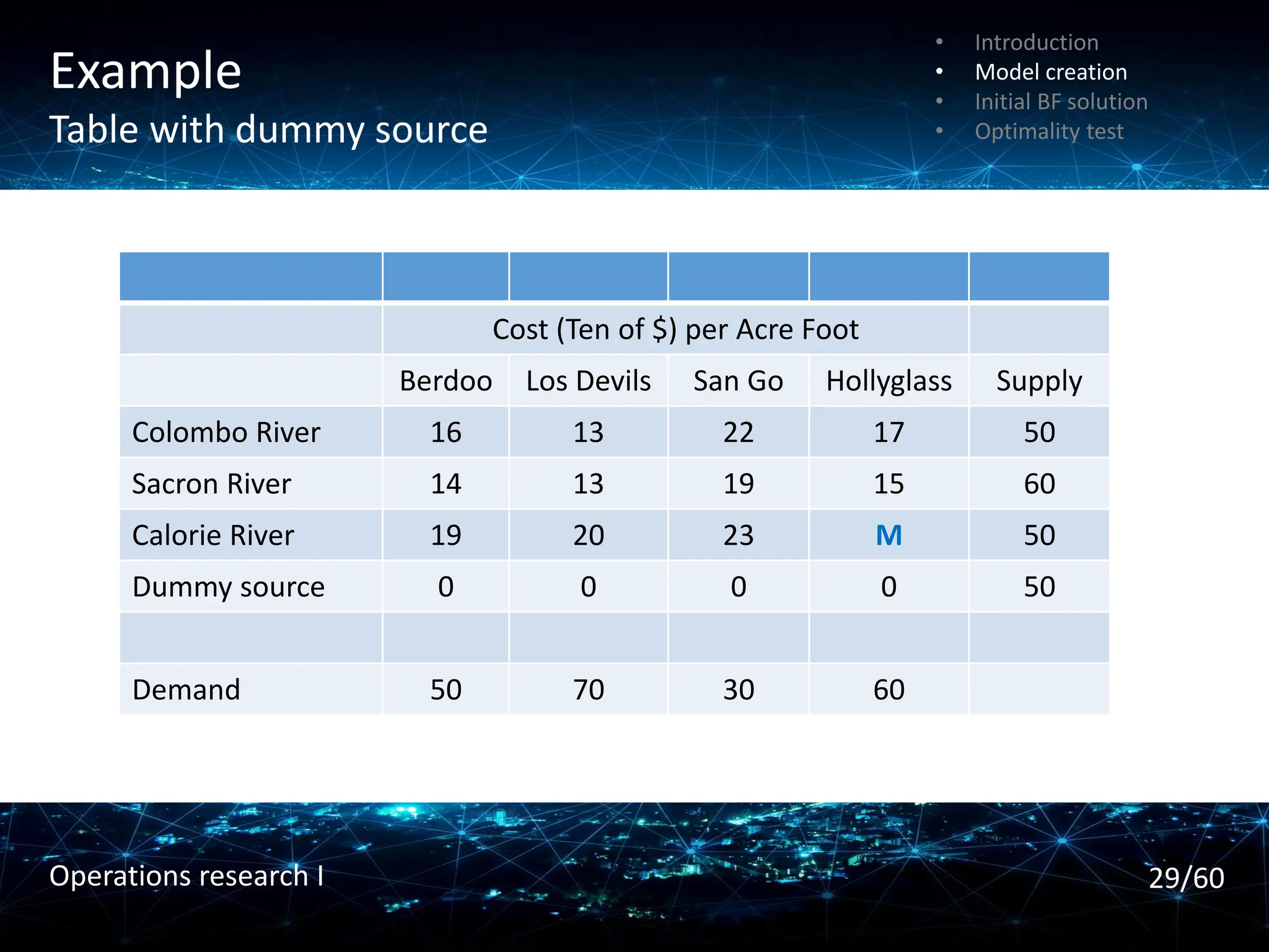
29. Example
Table with dummy source
Cost (Ten of $) per Acre Foot
Berdoo Los Devils San Go Hollyglass Supply
Colombo River 16 13 22 17 50
Sacron River 14 13 19 15 60
Calorie River 19 20 23 M 50
Dummy source 0 0 0 0 50
Demand 50 70 30 60
• Introduction
• Model creation
• Initial BF solution
• Optimality test
29/60
Operations research I

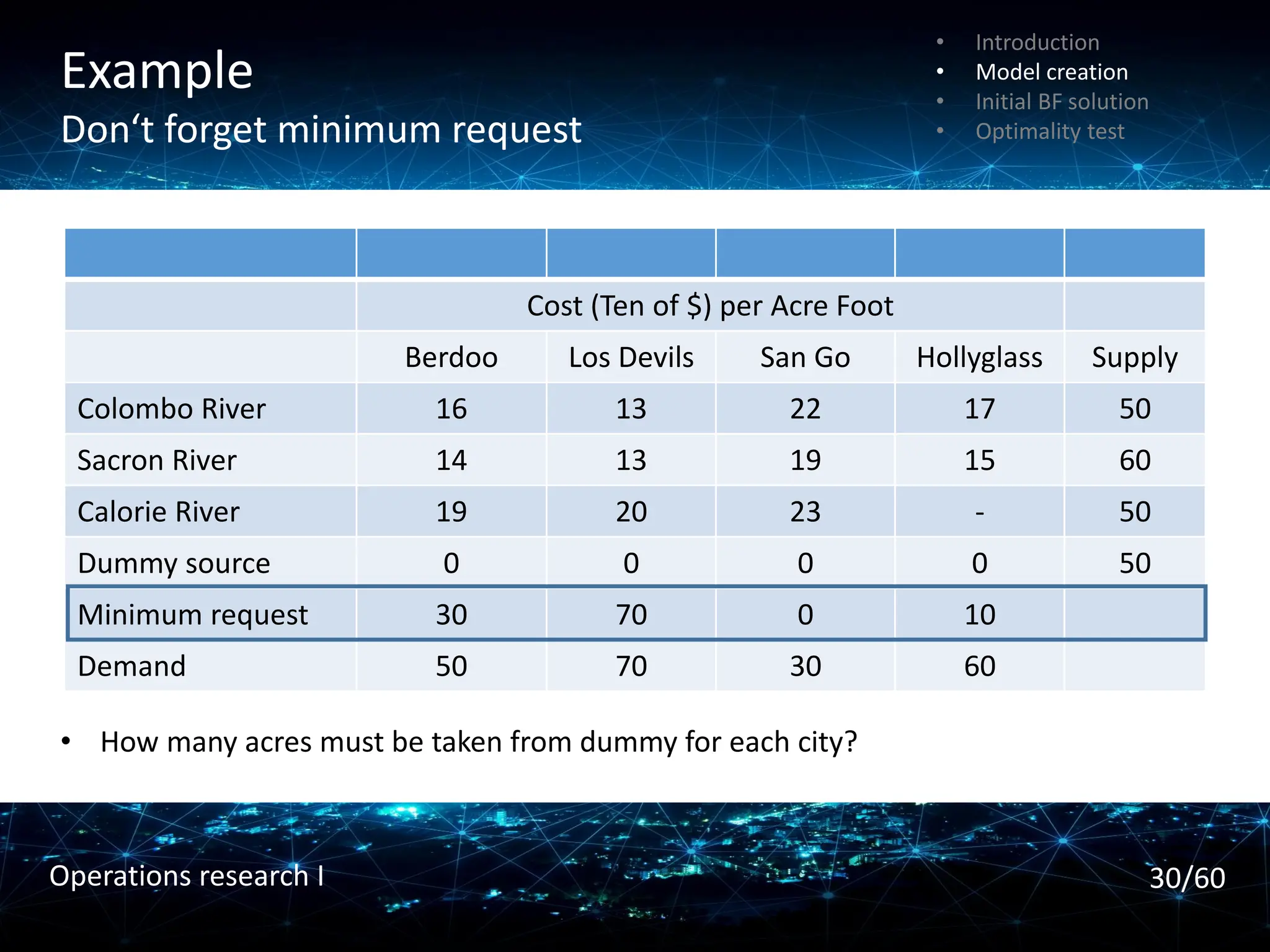
30. Example
Don‘t forget minimum request
Cost (Ten of $) per Acre Foot
Berdoo Los Devils San Go Hollyglass Supply
Colombo River 16 13 22 17 50
Sacron River 14 13 19 15 60
Calorie River 19 20 23 - 50
Dummy source 0 0 0 0 50
Minimum request 30 70 0 10
Demand 50 70 30 60
• How many acres must be taken from dummy for each city?
• Introduction
• Model creation
• Initial BF solution
• Optimality test
30/60
Operations research I

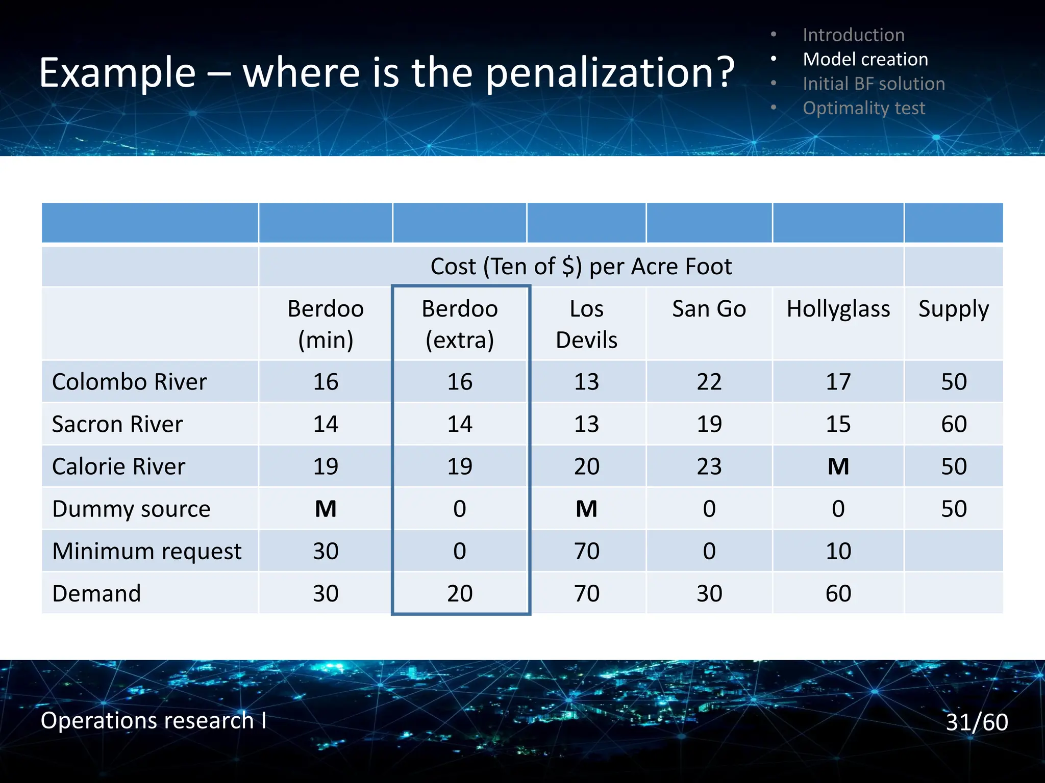
31. Example – where is the penalization?
Cost (Ten of $) per Acre Foot
Berdoo
(min)
Berdoo
(extra)
Los
Devils
San Go Hollyglass Supply
Colombo River 16 16 13 22 17 50
Sacron River 14 14 13 19 15 60
Calorie River 19 19 20 23 M 50
Dummy source M 0 M 0 0 50
Minimum request 30 0 70 0 10
Demand 30 20 70 30 60
• Introduction
• Model creation
• Initial BF solution
• Optimality test
31/60
Operations research I

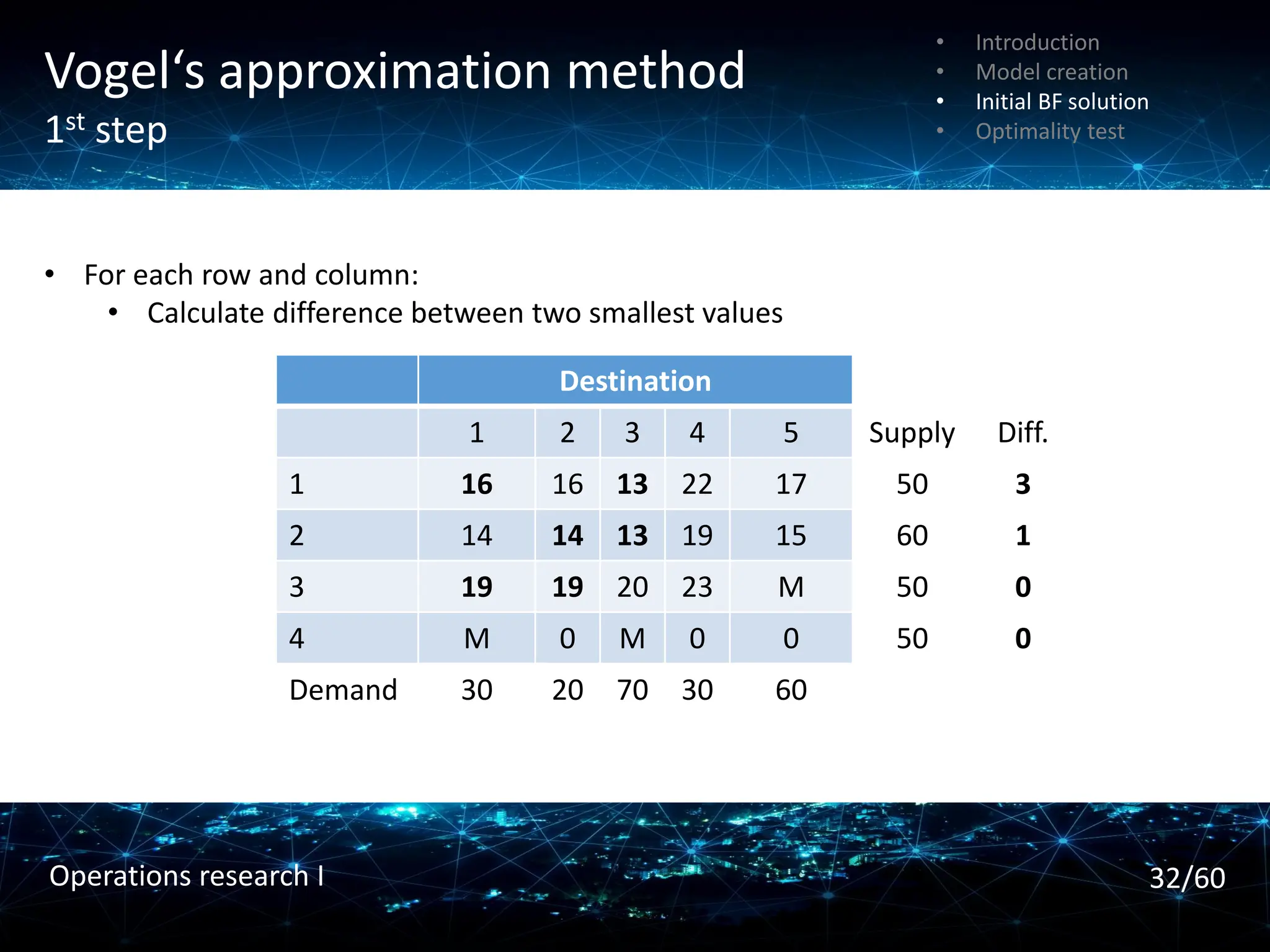
32. Vogel‘s approximation method
1st step
• For each row and column:
• Calculate difference between two smallest values
Destination
1 2 3 4 5 Supply Diff.
1 16 16 13 22 17 50 3
2 14 14 13 19 15 60 1
3 19 19 20 23 M 50 0
4 M 0 M 0 0 50 0
Demand 30 20 70 30 60
• Introduction
• Model creation
• Initial BF solution
• Optimality test
32/60
Operations research I

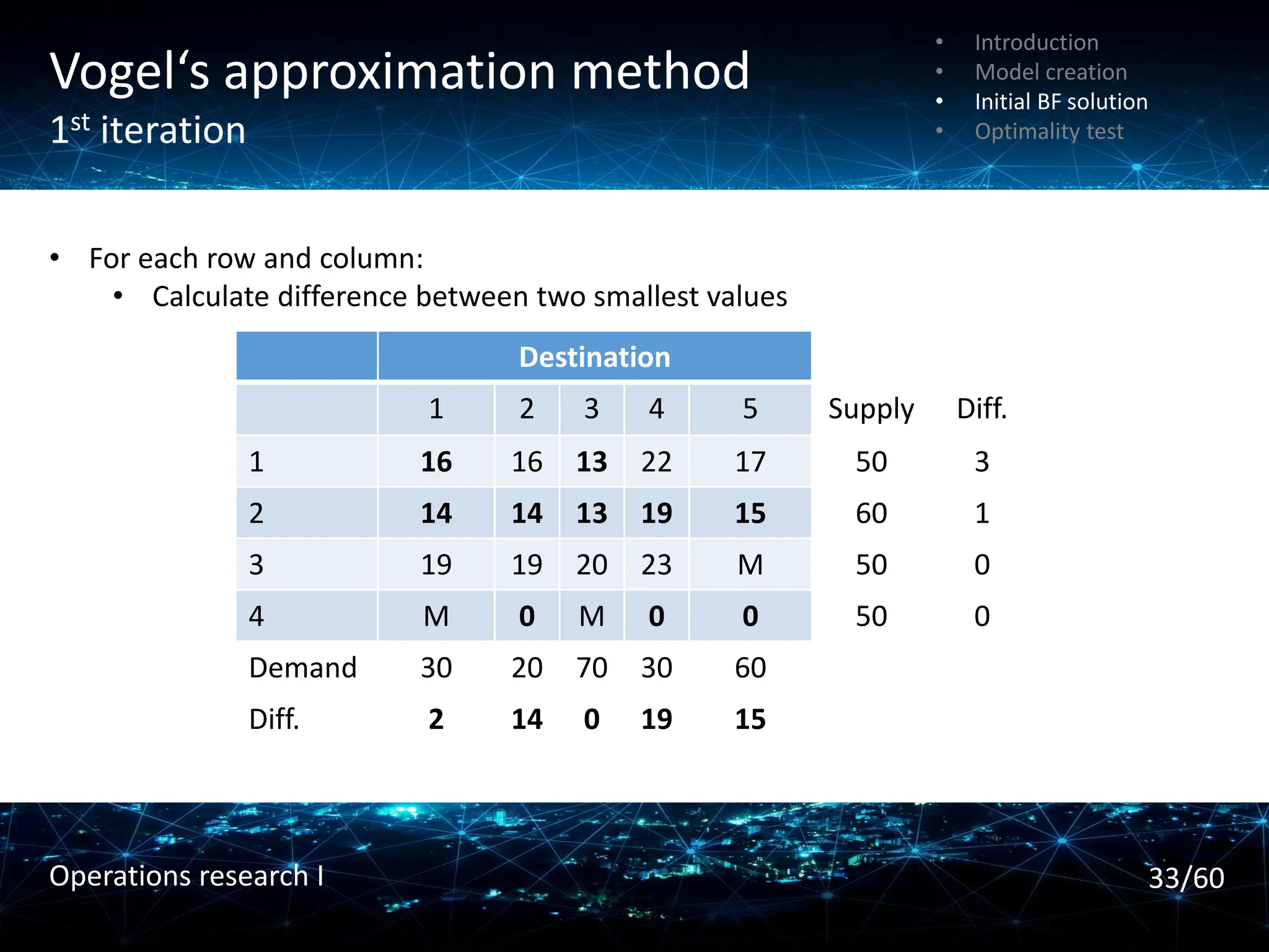
33. Vogel‘s approximation method
1st iteration
• For each row and column:
• Calculate difference between two smallest values
Destination
1 2 3 4 5 Supply Diff.
1 16 16 13 22 17 50 3
2 14 14 13 19 15 60 1
3 19 19 20 23 M 50 0
4 M 0 M 0 0 50 0
Demand 30 20 70 30 60
Diff. 2 14 0 19 15
• Introduction
• Model creation
• Initial BF solution
• Optimality test
33/60
Operations research I

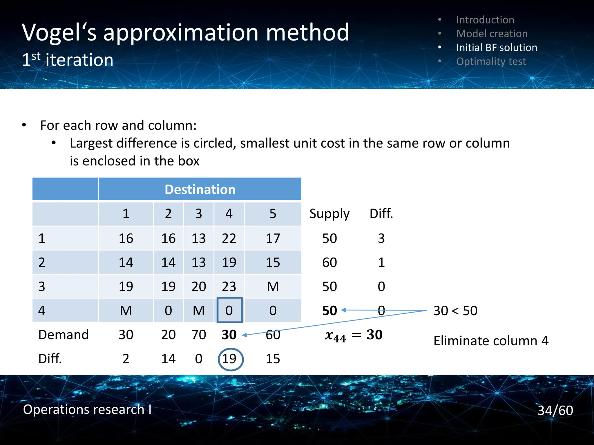
34. Vogel‘s approximation method
1st iteration
• For each row and column:
• Largest difference is circled, smallest unit cost in the same row or column
is enclosed in the box
Destination
1 2 3 4 5 Supply Diff.
1 16 16 13 22 17 50 3
2 14 14 13 19 15 60 1
3 19 19 20 23 M 50 0
4 M 0 M 0 0 50 0
Demand 30 20 70 30 60 𝒙𝟒𝟒 = 𝟑0
Diff. 2 14 0 19 15
Eliminate column 4
30 < 50
• Introduction
• Model creation
• Initial BF solution
• Optimality test
34/60
Operations research I

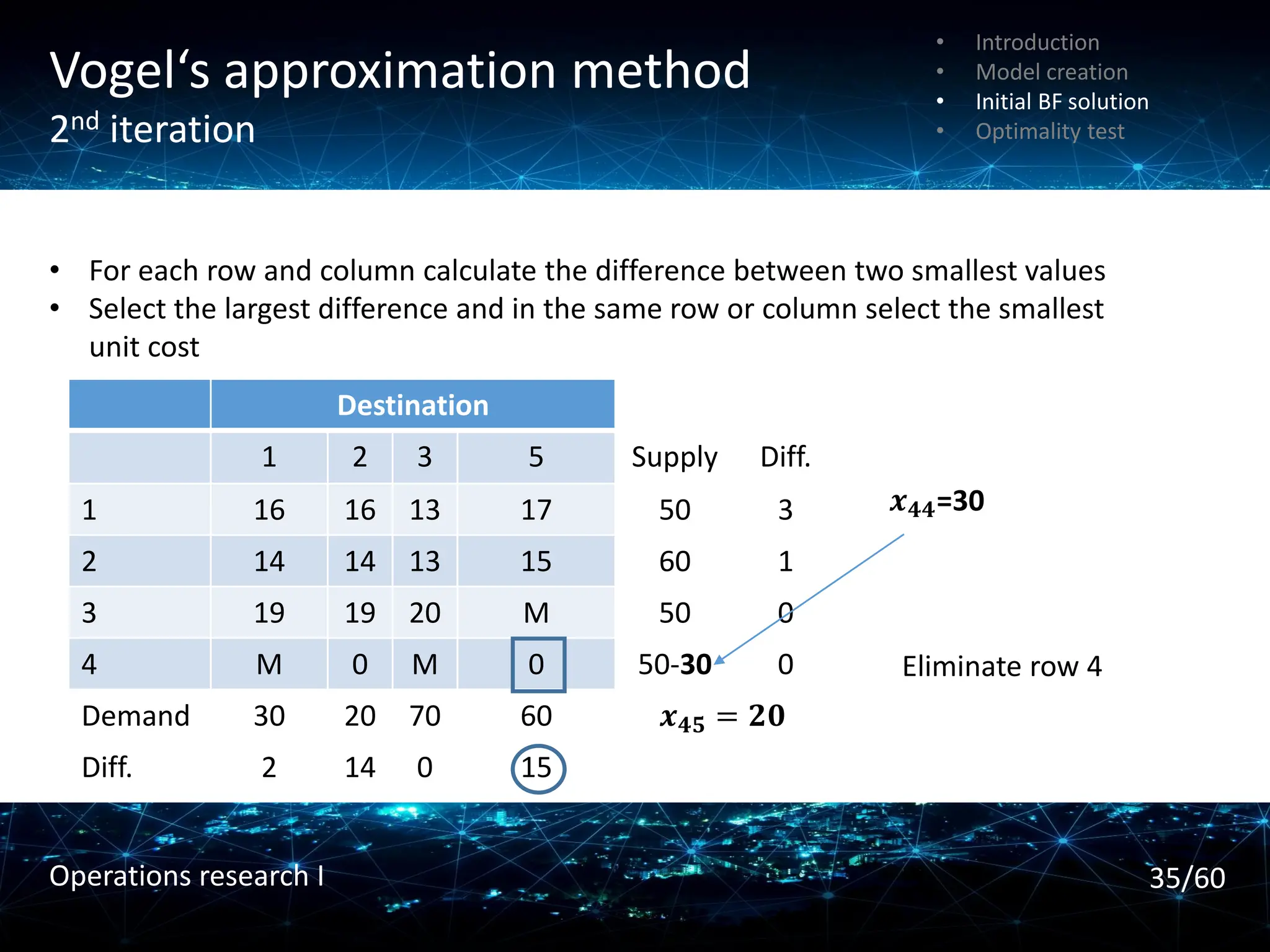
35. Vogel‘s approximation method
2nd iteration
• For each row and column calculate the difference between two smallest values
• Select the largest difference and in the same row or column select the smallest
unit cost
Destination
1 2 3 5 Supply Diff.
1 16 16 13 17 50 3
2 14 14 13 15 60 1
3 19 19 20 M 50 0
4 M 0 M 0 50-30 0
Demand 30 20 70 60 𝒙𝟒𝟓 = 𝟐𝟎
Diff. 2 14 0 15
Eliminate row 4
𝒙𝟒𝟒=30
• Introduction
• Model creation
• Initial BF solution
• Optimality test
35/60
Operations research I

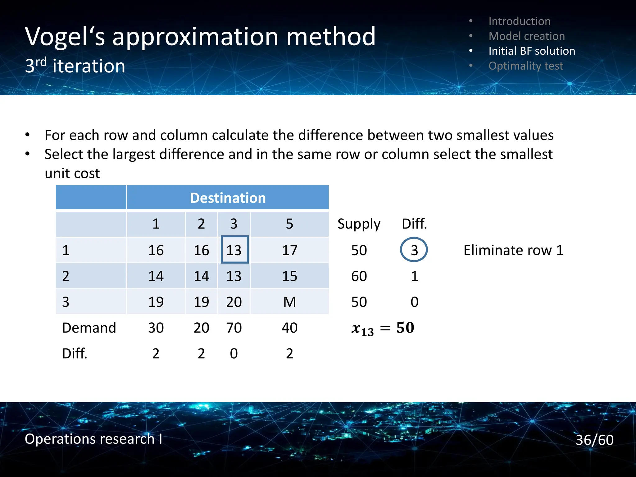
36. Vogel‘s approximation method
3rd iteration
• For each row and column calculate the difference between two smallest values
• Select the largest difference and in the same row or column select the smallest
unit cost
Destination
1 2 3 5 Supply Diff.
1 16 16 13 17 50 3
2 14 14 13 15 60 1
3 19 19 20 M 50 0
Demand 30 20 70 40 𝒙𝟏𝟑 = 𝟓𝟎
Diff. 2 2 0 2
Eliminate row 1
• Introduction
• Model creation
• Initial BF solution
• Optimality test
36/60
Operations research I

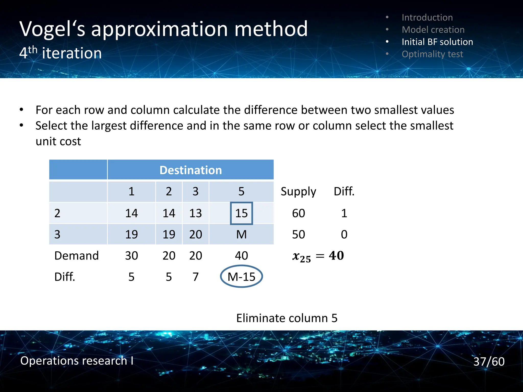
37. Vogel‘s approximation method
4th iteration
• For each row and column calculate the difference between two smallest values
• Select the largest difference and in the same row or column select the smallest
unit cost
Destination
1 2 3 5 Supply Diff.
2 14 14 13 15 60 1
3 19 19 20 M 50 0
Demand 30 20 20 40 𝒙𝟐𝟓 = 𝟒𝟎
Diff. 5 5 7 M-15
Eliminate column 5
• Introduction
• Model creation
• Initial BF solution
• Optimality test
37/60
Operations research I

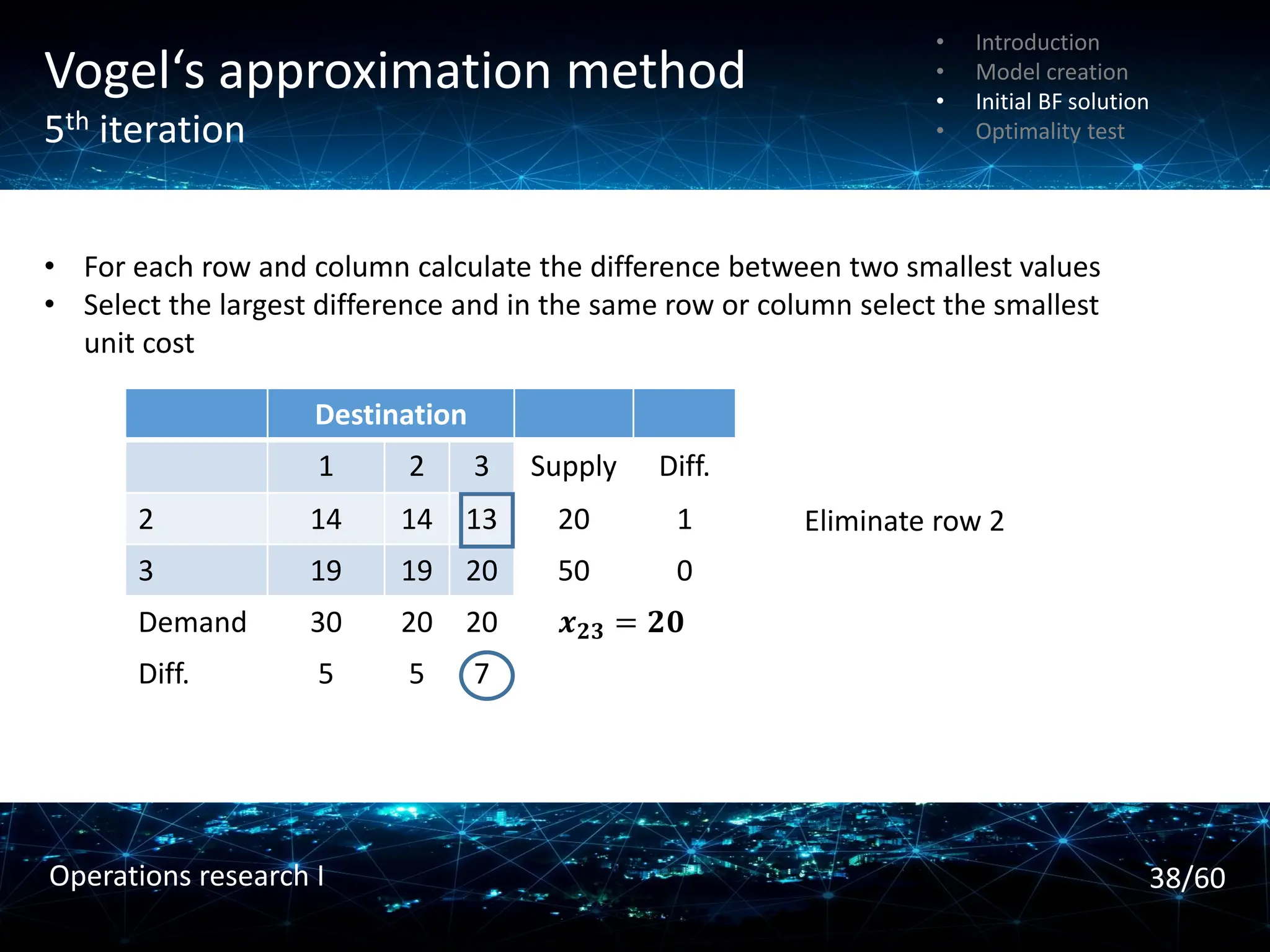
38. Vogel‘s approximation method
5th iteration
• For each row and column calculate the difference between two smallest values
• Select the largest difference and in the same row or column select the smallest
unit cost
Destination
1 2 3 Supply Diff.
2 14 14 13 20 1
3 19 19 20 50 0
Demand 30 20 20 𝒙𝟐𝟑 = 𝟐𝟎
Diff. 5 5 7
Eliminate row 2
• Introduction
• Model creation
• Initial BF solution
• Optimality test
38/60
Operations research I

39. Vogel‘s approximation method
solution
Destination
1 2 3 Supply Diff.
3 19 19 20 50 0
Demand 30 20 0 𝒙𝟑𝟐 = 𝟑𝟎
𝒙𝟑𝟐 = 𝟐𝟎
𝒙𝟑𝟑 = 𝟎
Diff. 5 5 7
𝒙𝟒𝟒 = 𝟑𝟎
𝒙𝟒𝟓 = 𝟐𝟎
𝒙𝟏𝟑 = 𝟓𝟎
𝒙𝟐𝟓 = 𝟒𝟎
𝒙𝟐𝟑 = 𝟐𝟎
𝒙𝟑𝟏 = 𝟑𝟎
𝒙𝟑𝟐 = 𝟐𝟎
𝒙𝟑𝟑 = 𝟎
Variable values:
𝑍 = 0 ∗ 30 + 0 ∗ 20 + 13 ∗ 50 + 15 ∗ 40 + 13 ∗ 20 + 19 ∗ 30 + 19 ∗ 20 + 20 ∗ 0
𝑍 = 0 + 0 + 650 + 600 + 260 + 570 + 380 + 0 = 𝟐𝟒𝟔𝟎
The value of the remaining variables is 0
𝒙𝟒𝟒 = 𝟑𝟎
𝒙𝟒𝟓 = 𝟐𝟎
𝒙𝟏𝟑 = 𝟓𝟎
𝒙𝟐𝟓 = 𝟒𝟎
𝒙𝟐𝟑 = 𝟐𝟎
𝒙𝟑𝟏 = 𝟑𝟎
𝒙𝟑𝟐 = 𝟐𝟎
𝒙𝟑𝟑 = 𝟎
• Introduction
• Model creation
• Initial BF solution
• Optimality test
39/60
Operations research I

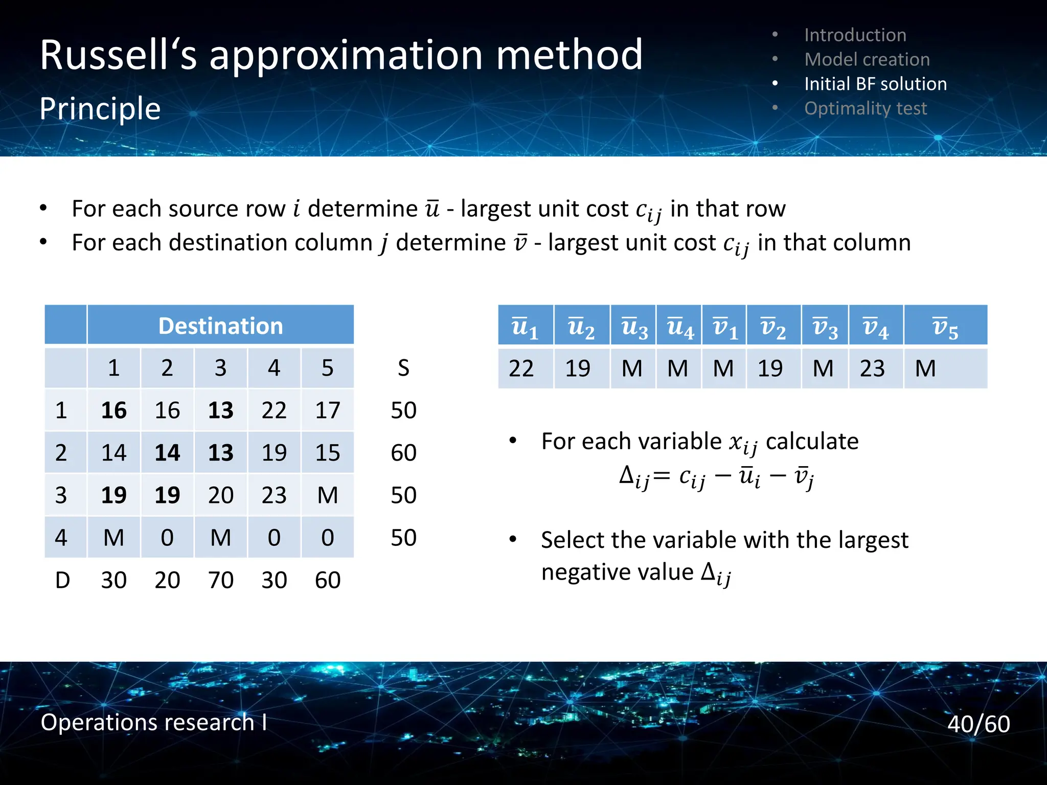
40. Russell‘s approximation method
Principle
Destination
1 2 3 4 5 S
1 16 16 13 22 17 50
2 14 14 13 19 15 60
3 19 19 20 23 M 50
4 M 0 M 0 0 50
D 30 20 70 30 60
• For each source row 𝑖 determine ത
𝑢 - largest unit cost 𝑐𝑖𝑗 in that row
• For each destination column 𝑗 determine ҧ
𝑣 - largest unit cost 𝑐𝑖𝑗 in that column
ഥ
𝒖𝟏 ഥ
𝒖𝟐 ഥ
𝒖𝟑 ഥ
𝒖𝟒 ഥ
𝒗𝟏 ഥ
𝒗𝟐 ഥ
𝒗𝟑 ഥ
𝒗𝟒 ഥ
𝒗𝟓
22 19 M M M 19 M 23 M
• For each variable 𝑥𝑖𝑗 calculate
∆𝑖𝑗= 𝑐𝑖𝑗 − ത
𝑢𝑖 − ҧ
𝑣𝑗
• Select the variable with the largest
negative value ∆𝑖𝑗
• Introduction
• Model creation
• Initial BF solution
• Optimality test
40/60
Operations research I

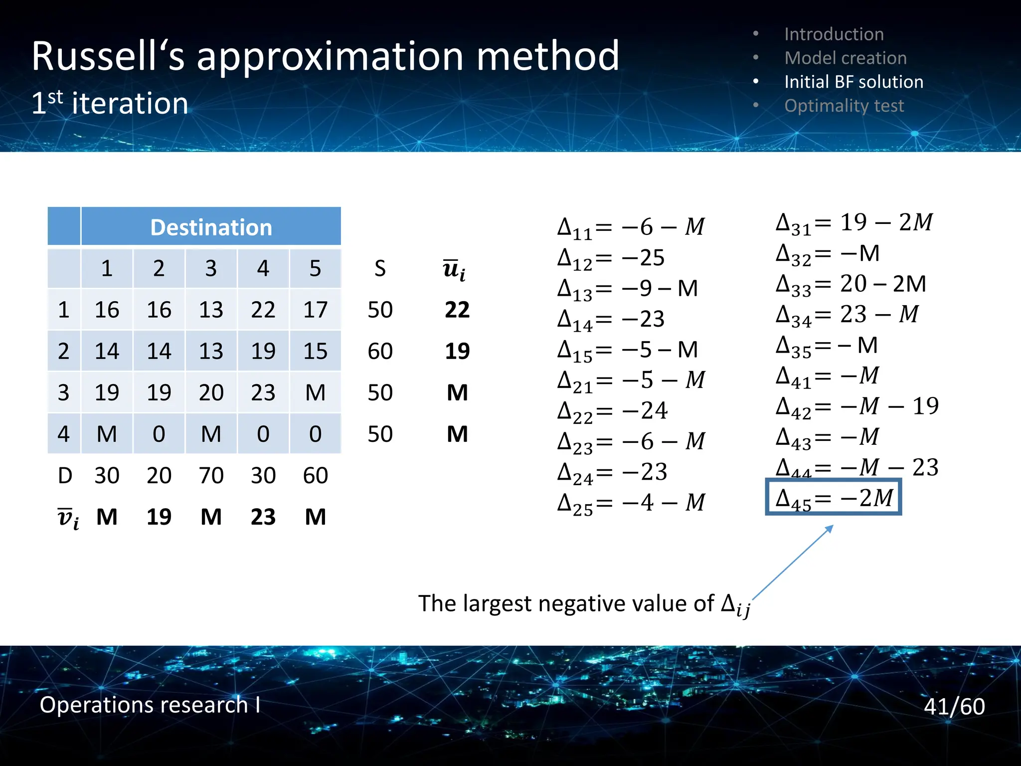
41. Russell‘s approximation method
1st iteration
Destination
1 2 3 4 5 S ഥ
𝒖𝒊
1 16 16 13 22 17 50 22
2 14 14 13 19 15 60 19
3 19 19 20 23 M 50 M
4 M 0 M 0 0 50 M
D 30 20 70 30 60
ഥ
𝒗𝒊 M 19 M 23 M
∆11= −6 − 𝑀
∆12= −25
∆13= −9 – M
∆14= −23
∆15= −5 – M
∆21= −5 − 𝑀
∆22= −24
∆23= −6 − 𝑀
∆24= −23
∆25= −4 − 𝑀
∆31= 19 − 2𝑀
∆32= −M
∆33= 20 – 2M
∆34= 23 − 𝑀
∆35= – M
∆41= −𝑀
∆42= −𝑀 − 19
∆43= −𝑀
∆44= −𝑀 − 23
∆45= −2𝑀
The largest negative value of ∆𝑖𝑗
• Introduction
• Model creation
• Initial BF solution
• Optimality test
41/60
Operations research I

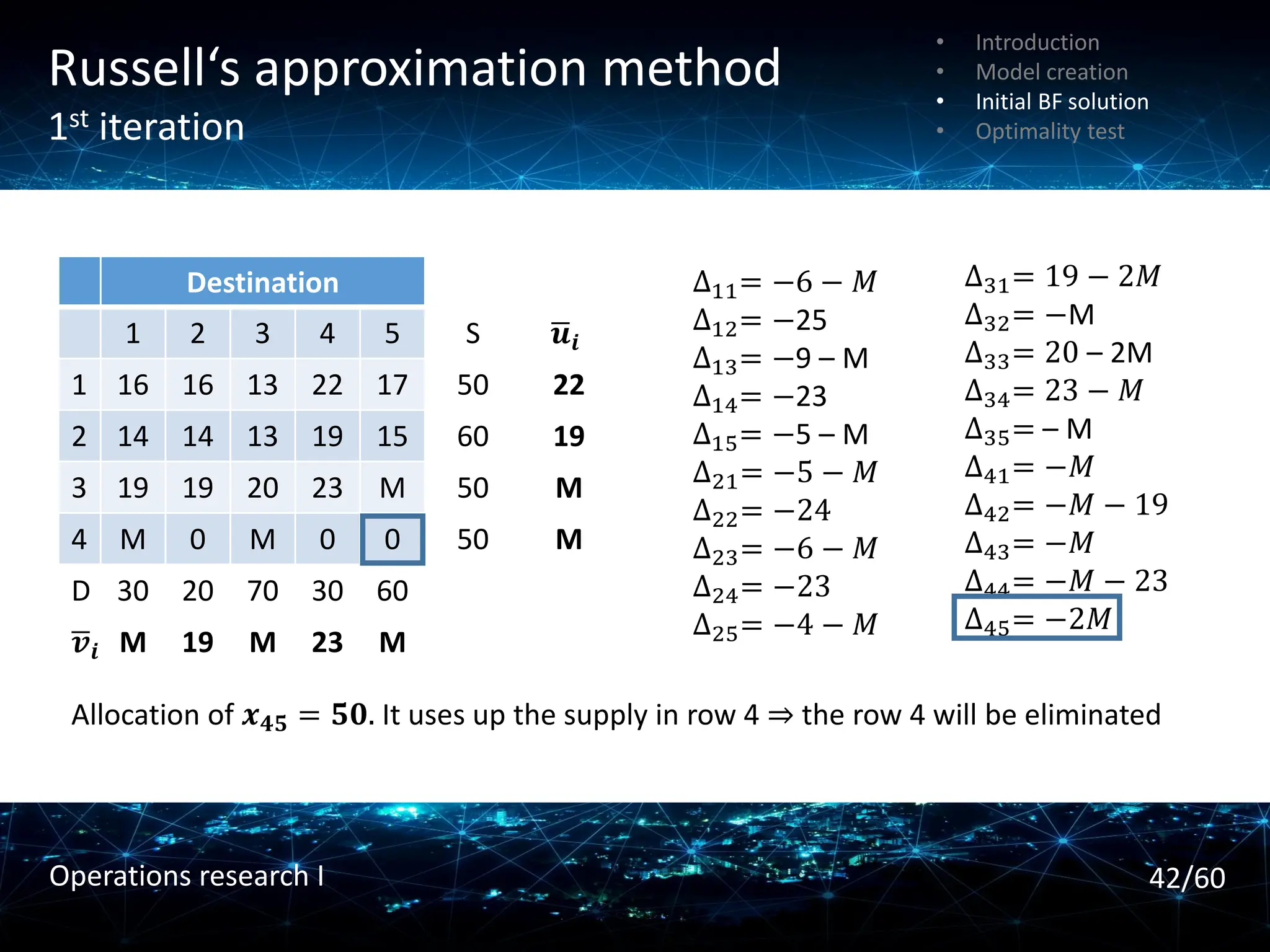
42. Russell‘s approximation method
1st iteration
Destination
1 2 3 4 5 S ഥ
𝒖𝒊
1 16 16 13 22 17 50 22
2 14 14 13 19 15 60 19
3 19 19 20 23 M 50 M
4 M 0 M 0 0 50 M
D 30 20 70 30 60
ഥ
𝒗𝒊 M 19 M 23 M
∆11= −6 − 𝑀
∆12= −25
∆13= −9 – M
∆14= −23
∆15= −5 – M
∆21= −5 − 𝑀
∆22= −24
∆23= −6 − 𝑀
∆24= −23
∆25= −4 − 𝑀
∆31= 19 − 2𝑀
∆32= −M
∆33= 20 – 2M
∆34= 23 − 𝑀
∆35= – M
∆41= −𝑀
∆42= −𝑀 − 19
∆43= −𝑀
∆44= −𝑀 − 23
∆45= −2𝑀
Allocation of 𝒙𝟒𝟓 = 𝟓𝟎. It uses up the supply in row 4 ⇒ the row 4 will be eliminated
• Introduction
• Model creation
• Initial BF solution
• Optimality test
42/60
Operations research I

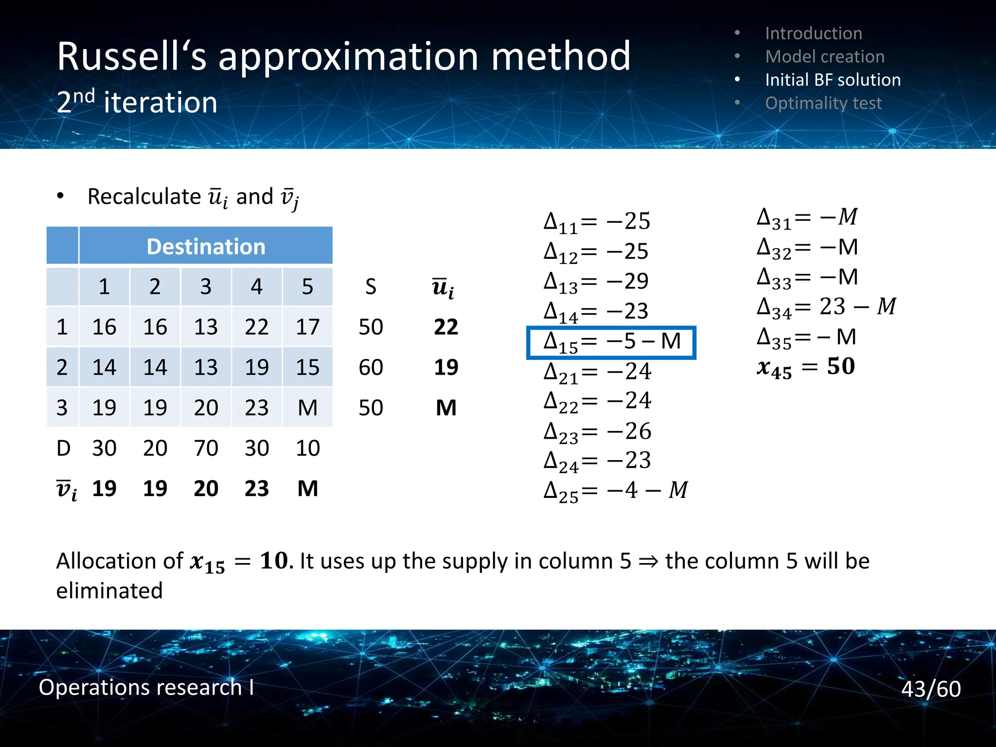
43. Russell‘s approximation method
2nd iteration
Destination
1 2 3 4 5 S ഥ
𝒖𝒊
1 16 16 13 22 17 50 22
2 14 14 13 19 15 60 19
3 19 19 20 23 M 50 M
D 30 20 70 30 10
ഥ
𝒗𝒊 19 19 20 23 M
∆11= −25
∆12= −25
∆13= −29
∆14= −23
∆15= −5 – M
∆21= −24
∆22= −24
∆23= −26
∆24= −23
∆25= −4 − 𝑀
∆31= −𝑀
∆32= −M
∆33= −M
∆34= 23 − 𝑀
∆35= – M
𝒙𝟒𝟓 = 𝟓𝟎
Allocation of 𝒙𝟏𝟓 = 𝟏𝟎. It uses up the supply in column 5 ⇒ the column 5 will be
eliminated
• Recalculate ത
𝑢𝑖 and ҧ
𝑣𝑗
• Introduction
• Model creation
• Initial BF solution
• Optimality test
43/60
Operations research I

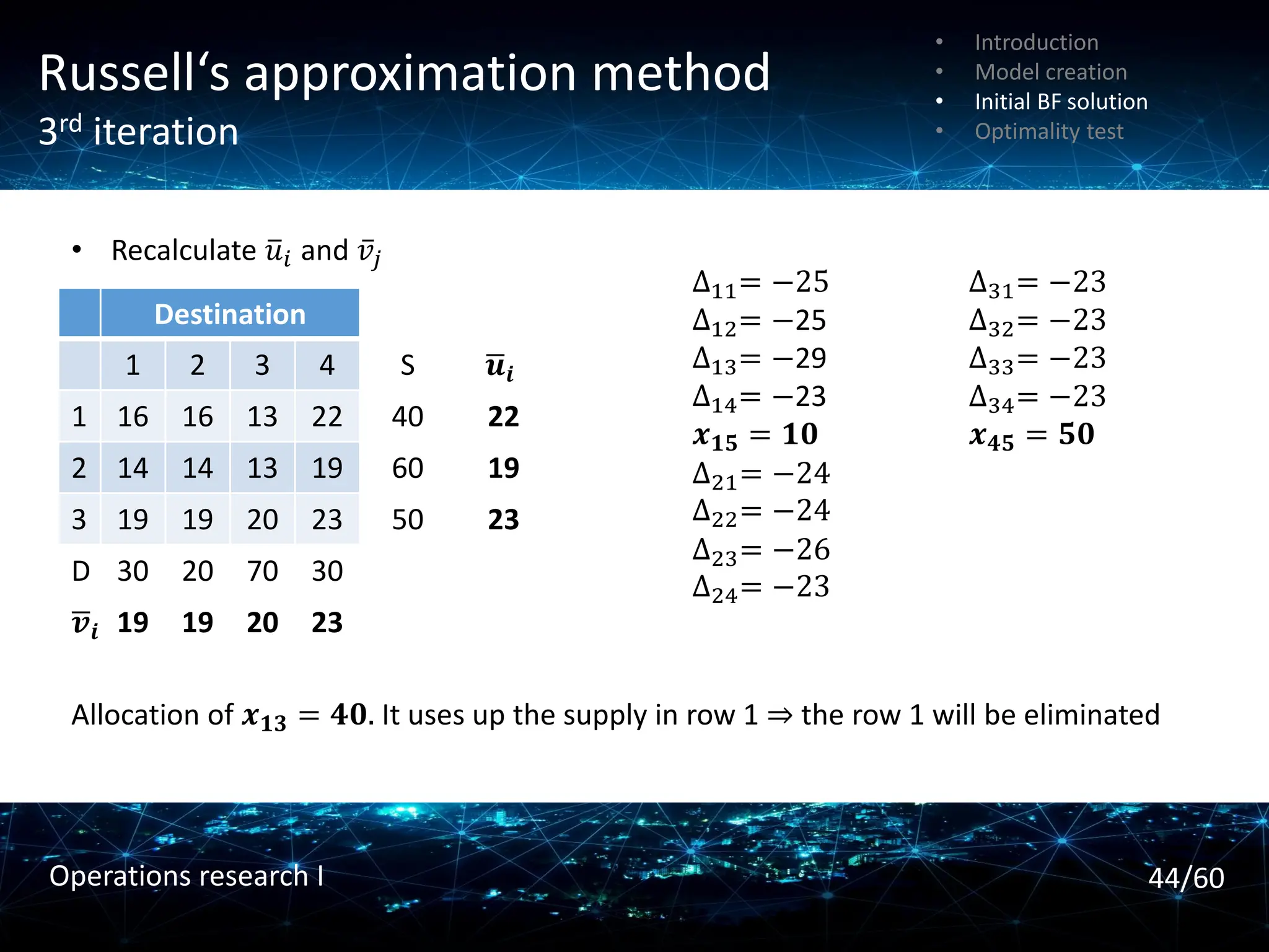
44. Russell‘s approximation method
3rd iteration
Destination
1 2 3 4 S ഥ
𝒖𝒊
1 16 16 13 22 40 22
2 14 14 13 19 60 19
3 19 19 20 23 50 23
D 30 20 70 30
ഥ
𝒗𝒊 19 19 20 23
∆11= −25
∆12= −25
∆13= −29
∆14= −23
𝒙𝟏𝟓 = 𝟏𝟎
∆21= −24
∆22= −24
∆23= −26
∆24= −23
∆31= −23
∆32= −23
∆33= −23
∆34= −23
𝒙𝟒𝟓 = 𝟓𝟎
Allocation of 𝒙𝟏𝟑 = 𝟒𝟎. It uses up the supply in row 1 ⇒ the row 1 will be eliminated
• Recalculate ത
𝑢𝑖 and ҧ
𝑣𝑗
• Introduction
• Model creation
• Initial BF solution
• Optimality test
44/60
Operations research I

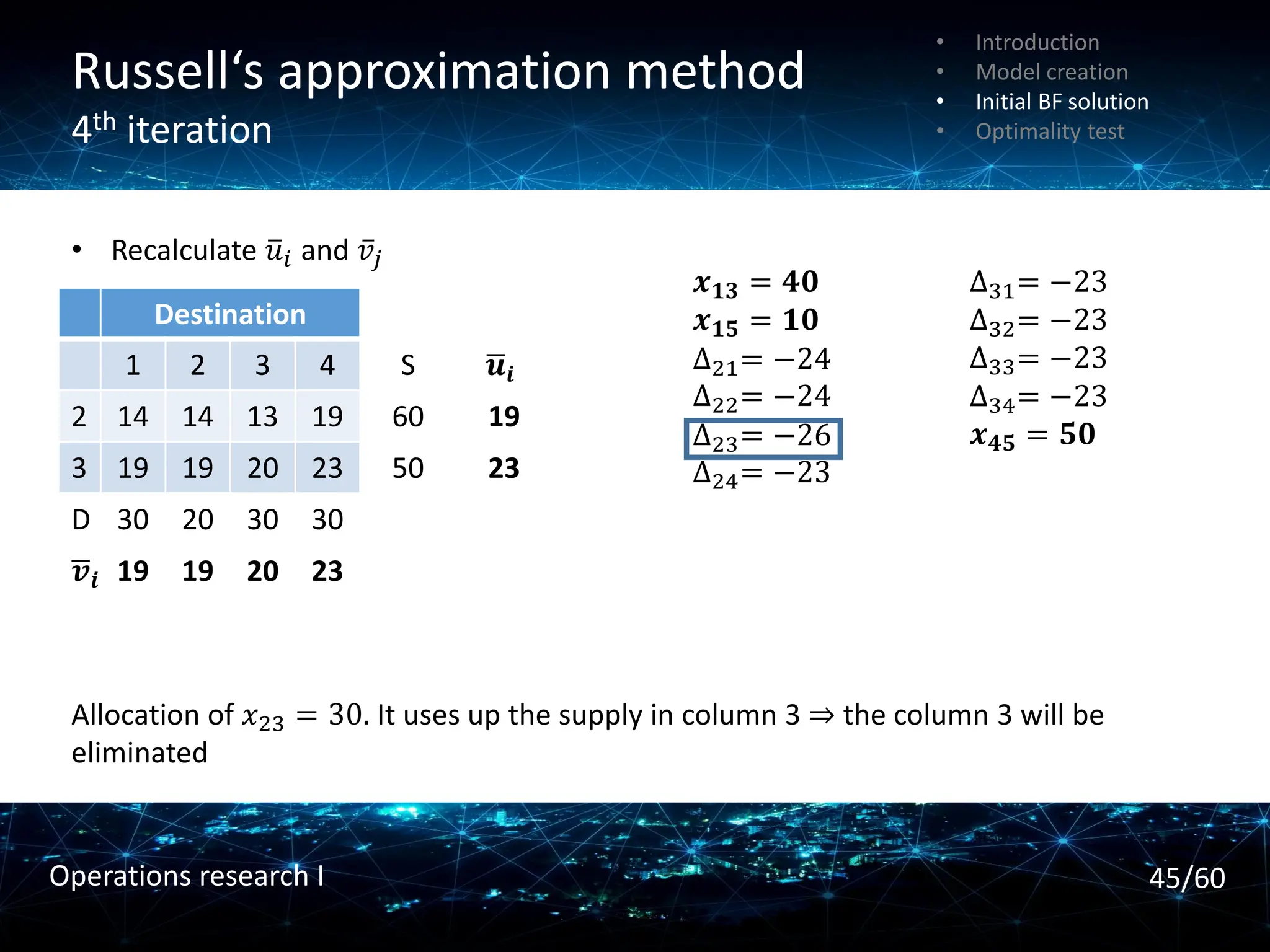
45. Russell‘s approximation method
4th iteration
Destination
1 2 3 4 S ഥ
𝒖𝒊
2 14 14 13 19 60 19
3 19 19 20 23 50 23
D 30 20 30 30
ഥ
𝒗𝒊 19 19 20 23
𝒙𝟏𝟑 = 𝟒𝟎
𝒙𝟏𝟓 = 𝟏𝟎
∆21= −24
∆22= −24
∆23= −26
∆24= −23
∆31= −23
∆32= −23
∆33= −23
∆34= −23
𝒙𝟒𝟓 = 𝟓𝟎
Allocation of 𝑥23 = 30. It uses up the supply in column 3 ⇒ the column 3 will be
eliminated
• Recalculate ത
𝑢𝑖 and ҧ
𝑣𝑗
• Introduction
• Model creation
• Initial BF solution
• Optimality test
45/60
Operations research I

46. Russell‘s approximation method
Result
𝒙𝟒𝟓 = 𝟓𝟎
𝒙𝟏𝟑 = 𝟒𝟎
𝒙𝟏𝟓 = 𝟏𝟎
𝒙𝟐𝟑 = 𝟑𝟎
𝒙𝟐𝟏 = 𝟑𝟎
𝒙𝟑𝟏 = 𝟎
𝒙𝟑𝟐 = 𝟐𝟎
𝒙𝟑𝟒 = 𝟑𝟎
• Initial BF solution from
Russell‘s approximation:
Destination
1 2 3 4 5 S
1 16 16 13 22 17 50
2 14 14 13 19 15 60
3 19 19 20 23 M 50
4 M 0 M 0 0 50
D 30 20 70 30 60
𝑍 = 0 ∗ 50 + 13 ∗ 40 + 17 ∗ 10 + 13 ∗ 30 + 14 ∗ 30 + 19 ∗ 0 + 19 ∗ 20 + 23 ∗ 30
𝑍 = 0 + 520 + 170 + 390 + 420 + 0 + 380 + 690 = 𝟐𝟓𝟕𝟎
• Introduction
• Model creation
• Initial BF solution
• Optimality test
46/60
Operations research I

47. Russell‘s approximation method
Initial transportation simplex tableau
• Introduction
• Model creation
• Initial BF solution
• Optimality test
Iteration Destination
0 1 2 3 4 5 Supply 𝑢𝑖
Source
1 50
2 60
3 50
4(D) 50
Demand 30 20 70 30 60 𝑍 = 2570
𝑣𝑗
16 16 13 22 17
14 14 13 19 15
19 19 20 23 M
M 0 M 0 0
40 10
30
0 20 30
50
47/60
Operations research I

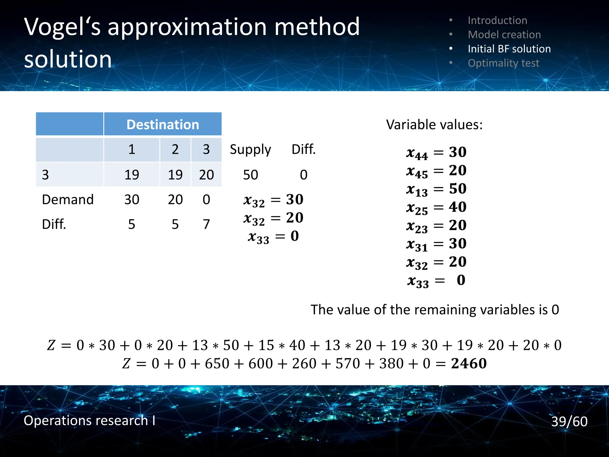
48. Russell‘s vs. Vogel‘s approximation
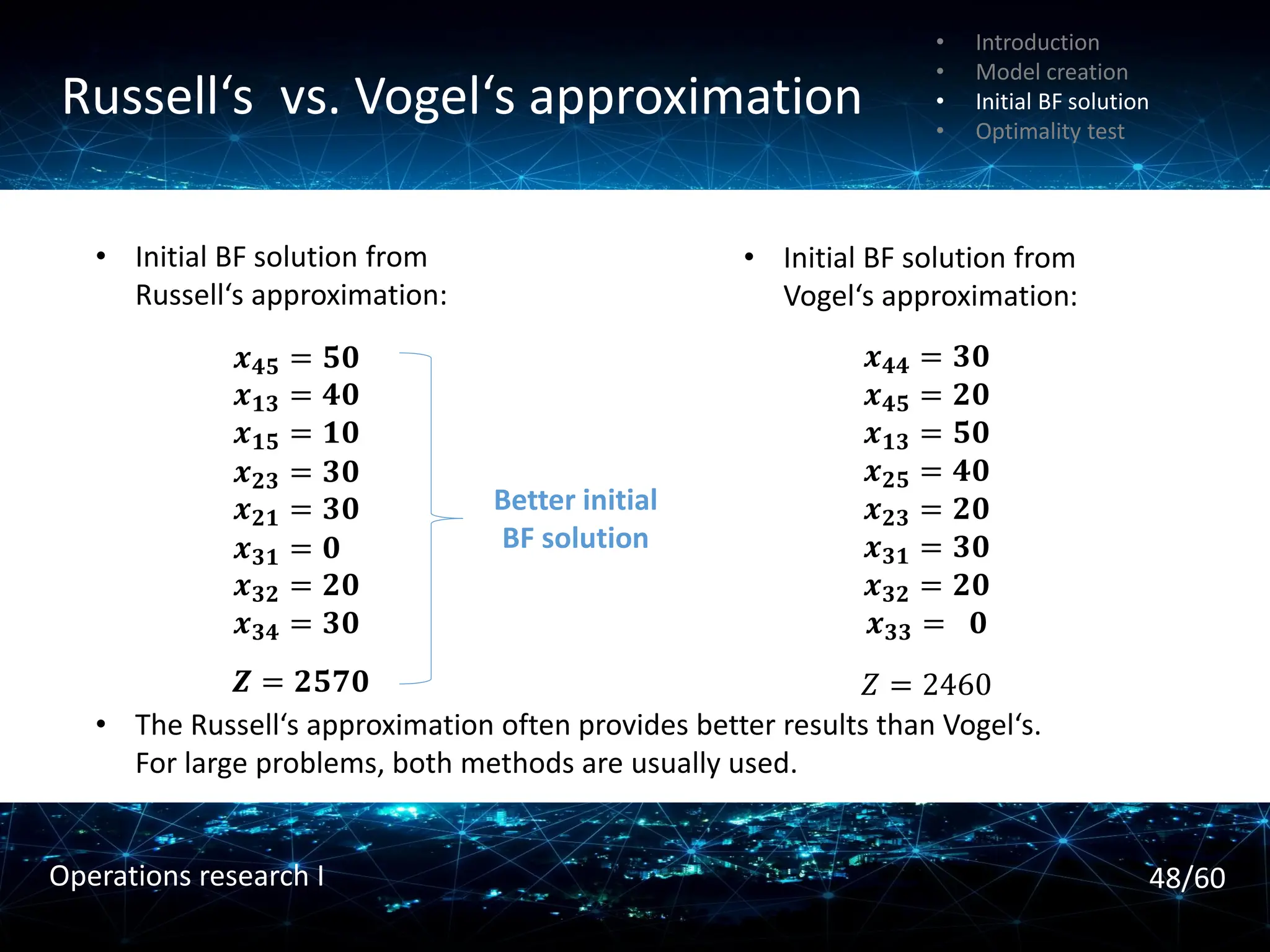
𝒙𝟒𝟓 = 𝟓𝟎
𝒙𝟏𝟑 = 𝟒𝟎
𝒙𝟏𝟓 = 𝟏𝟎
𝒙𝟐𝟑 = 𝟑𝟎
𝒙𝟐𝟏 = 𝟑𝟎
𝒙𝟑𝟏 = 𝟎
𝒙𝟑𝟐 = 𝟐𝟎
𝒙𝟑𝟒 = 𝟑𝟎
• Initial BF solution from
Russell‘s approximation:
• Initial BF solution from
Vogel‘s approximation:
𝒙𝟒𝟒 = 𝟑𝟎
𝒙𝟒𝟓 = 𝟐𝟎
𝒙𝟏𝟑 = 𝟓𝟎
𝒙𝟐𝟓 = 𝟒𝟎
𝒙𝟐𝟑 = 𝟐𝟎
𝒙𝟑𝟏 = 𝟑𝟎
𝒙𝟑𝟐 = 𝟐𝟎
𝒙𝟑𝟑 = 𝟎
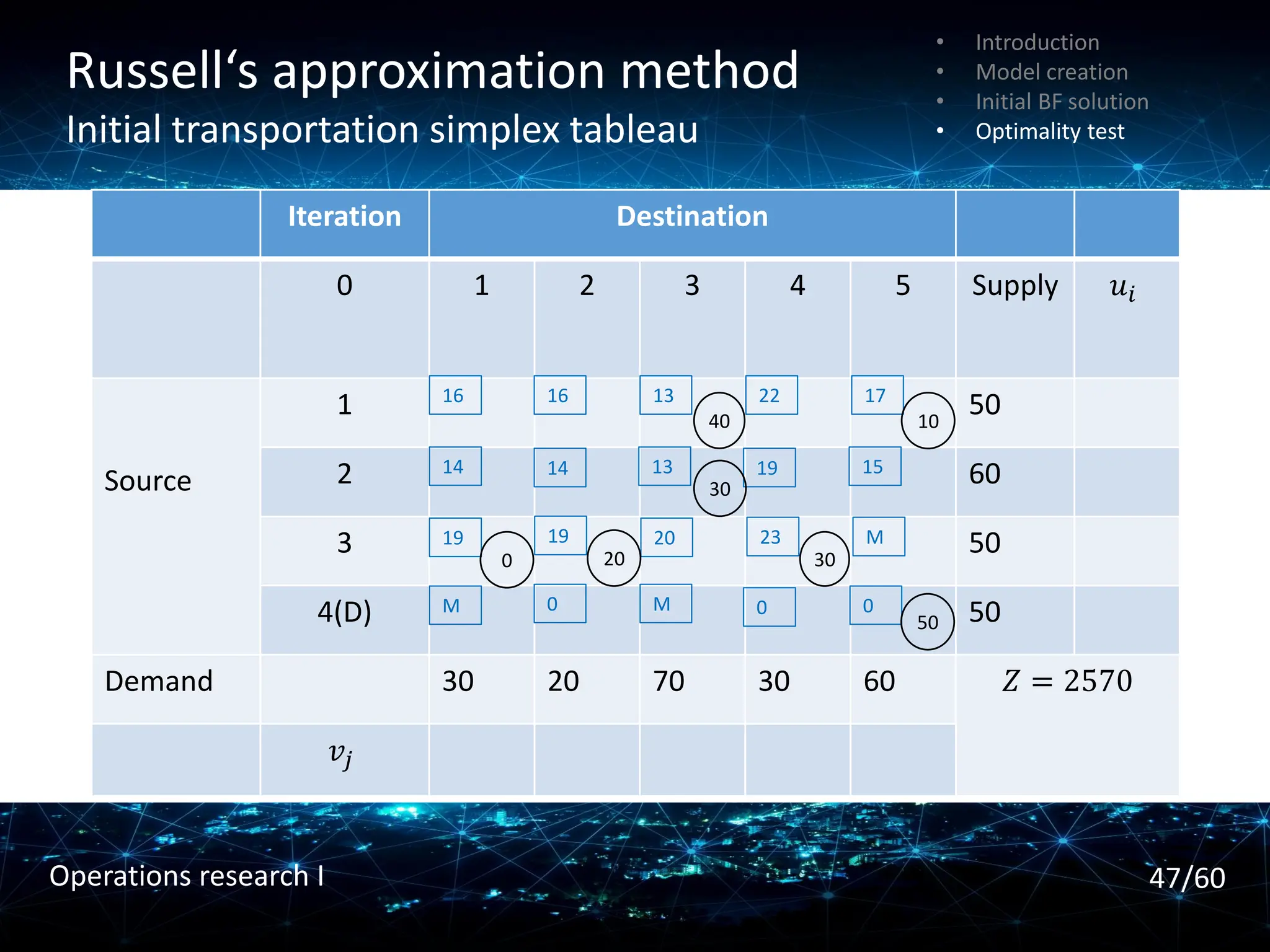
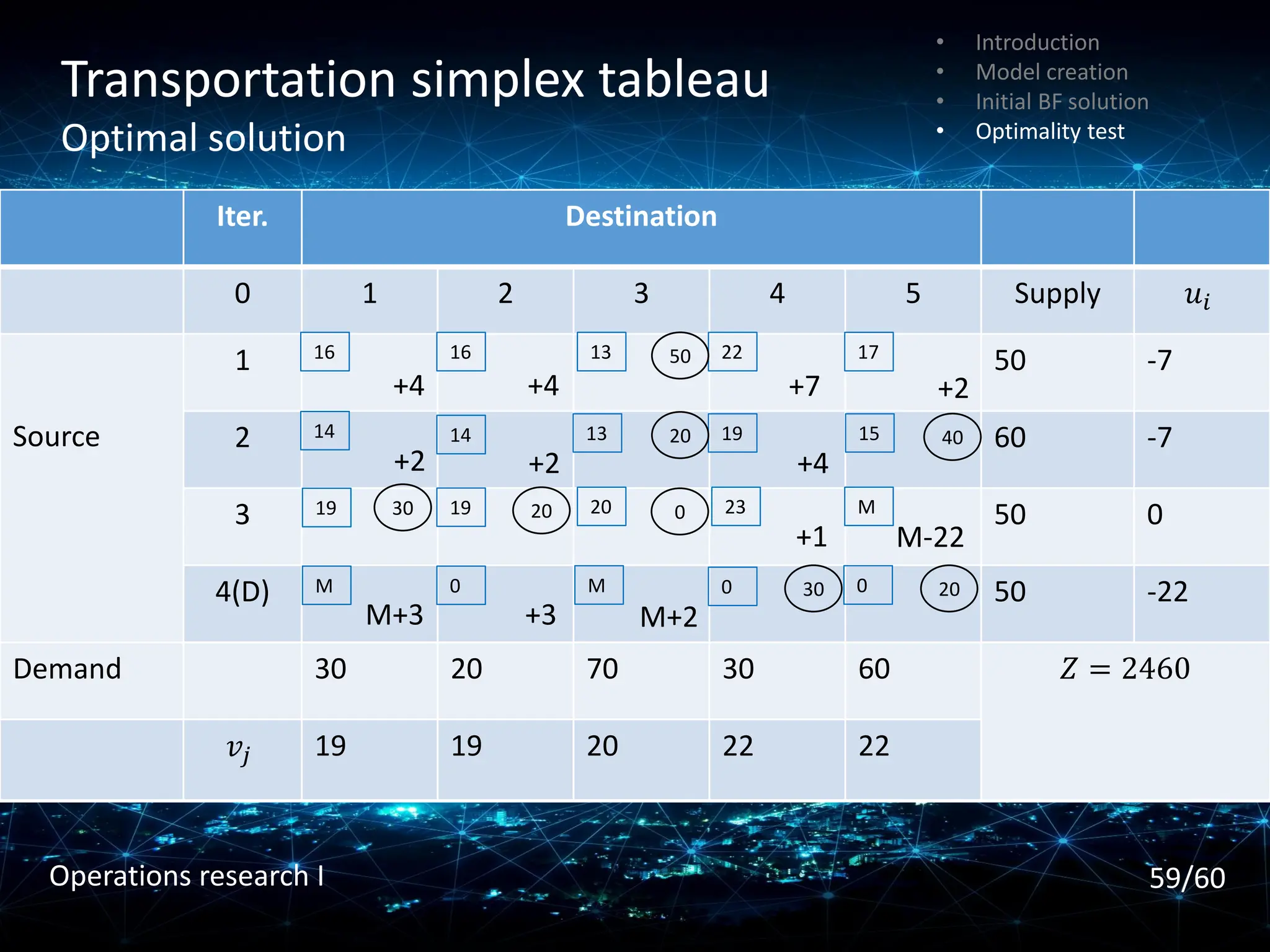
𝒁 = 𝟐𝟓𝟕𝟎 𝑍 = 2460
• The Russell‘s approximation often provides better results than Vogel‘s.
For large problems, both methods are usually used.
Better initial
BF solution
• Introduction
• Model creation
• Initial BF solution
• Optimality test
48/60
Operations research I

49. Optimality test
• Introduction
• Model creation
• Initial BF solution
• Optimality test
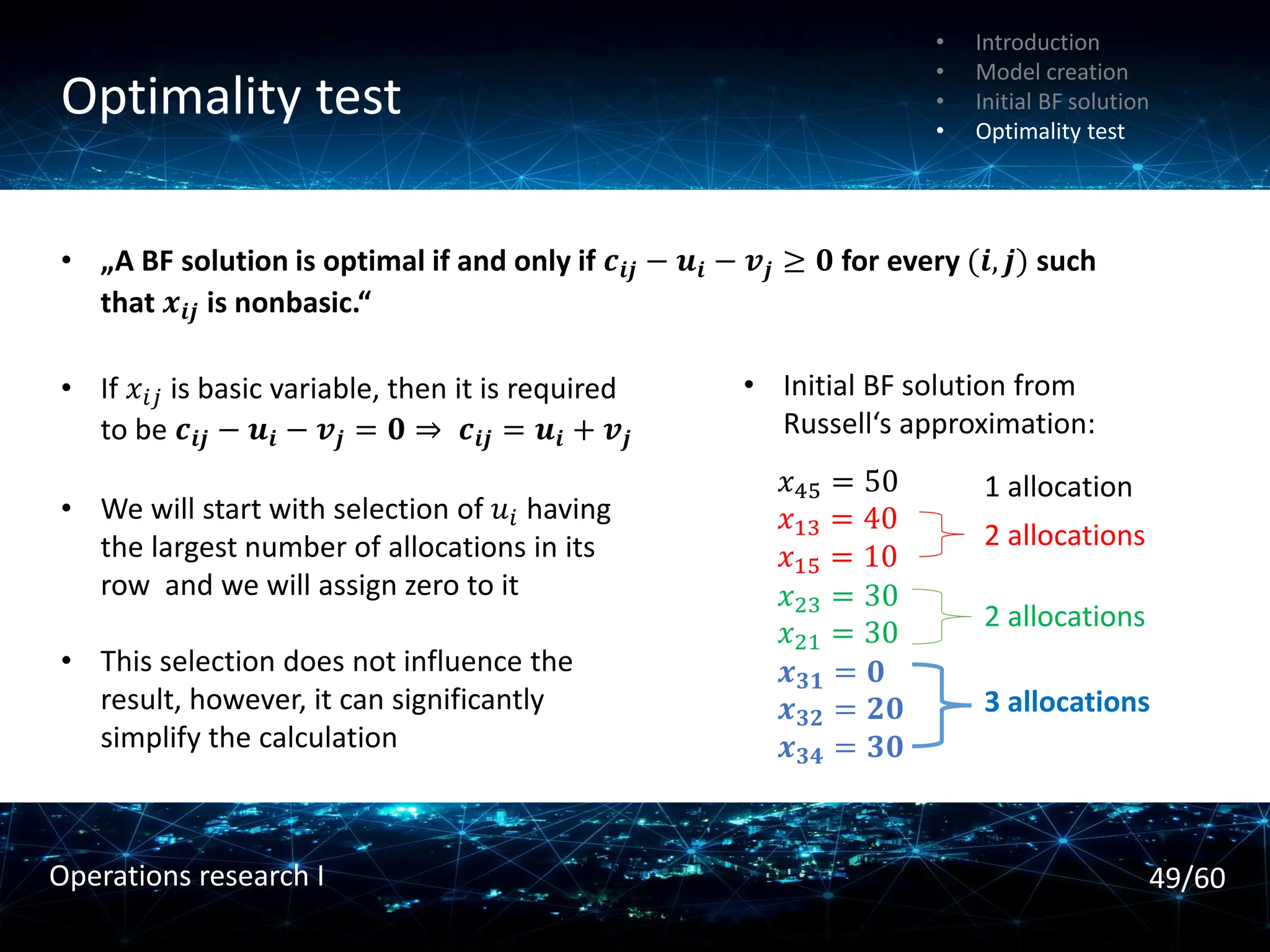
• „A BF solution is optimal if and only if 𝒄𝒊𝒋 − 𝒖𝒊 − 𝒗𝒋 ≥ 𝟎 for every (𝒊, 𝒋) such
that 𝒙𝒊𝒋 is nonbasic.“
• If 𝑥𝑖𝑗 is basic variable, then it is required
to be 𝒄𝒊𝒋 − 𝒖𝒊 − 𝒗𝒋 = 𝟎 ⇒ 𝒄𝒊𝒋 = 𝒖𝒊 + 𝒗𝒋
• We will start with selection of 𝑢𝑖 having
the largest number of allocations in its
row and we will assign zero to it
• This selection does not influence the
result, however, it can significantly
simplify the calculation
𝑥45 = 50
𝑥13 = 40
𝑥15 = 10
𝑥23 = 30
𝑥21 = 30
𝒙𝟑𝟏 = 𝟎
𝒙𝟑𝟐 = 𝟐𝟎
𝒙𝟑𝟒 = 𝟑𝟎
• Initial BF solution from
Russell‘s approximation:
3 allocations
2 allocations
2 allocations
1 allocation
49/60
Operations research I

50. Optimality test
• Introduction
• Model creation
• Initial BF solution
• Optimality test
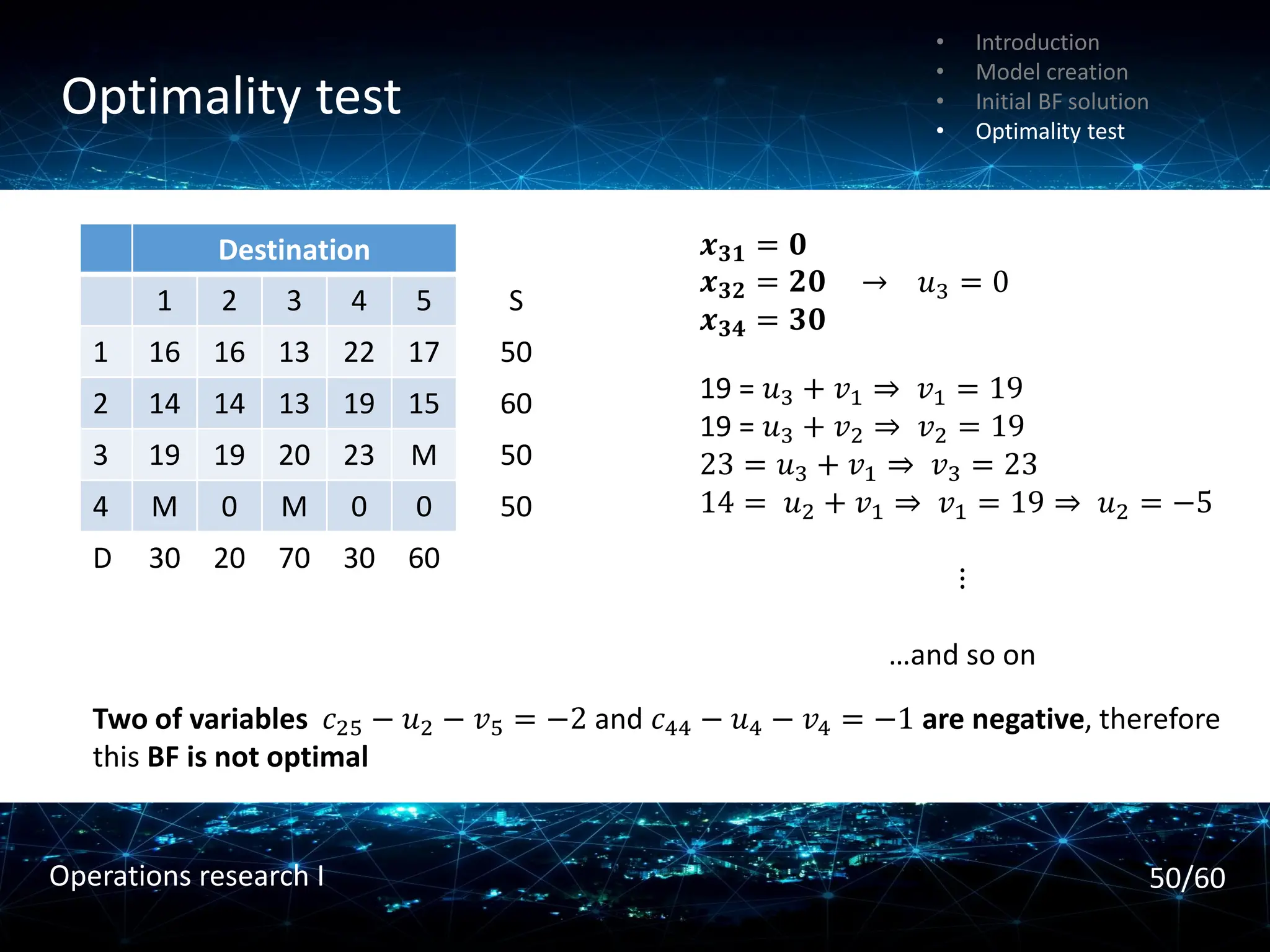
𝒙𝟑𝟏 = 𝟎
𝒙𝟑𝟐 = 𝟐𝟎
𝒙𝟑𝟒 = 𝟑𝟎
Destination
1 2 3 4 5 S
1 16 16 13 22 17 50
2 14 14 13 19 15 60
3 19 19 20 23 M 50
4 M 0 M 0 0 50
D 30 20 70 30 60
→ 𝑢3 = 0
19 = 𝑢3 + 𝑣1 ⇒ 𝑣1 = 19
19 = 𝑢3 + 𝑣2 ⇒ 𝑣2 = 19
23 = 𝑢3 + 𝑣1 ⇒ 𝑣3 = 23
14 = 𝑢2 + 𝑣1 ⇒ 𝑣1 = 19 ⇒ 𝑢2 = −5
⋮
…and so on
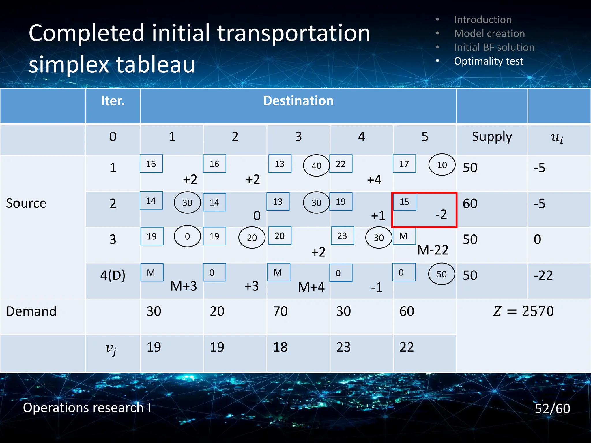
Two of variables 𝑐25 − 𝑢2 − 𝑣5 = −2 and 𝑐44 − 𝑢4 − 𝑣4 = −1 are negative, therefore
this BF is not optimal
50/60
Operations research I

51. An iteration
• Introduction
• Model creation
• Initial BF solution
• Optimality test
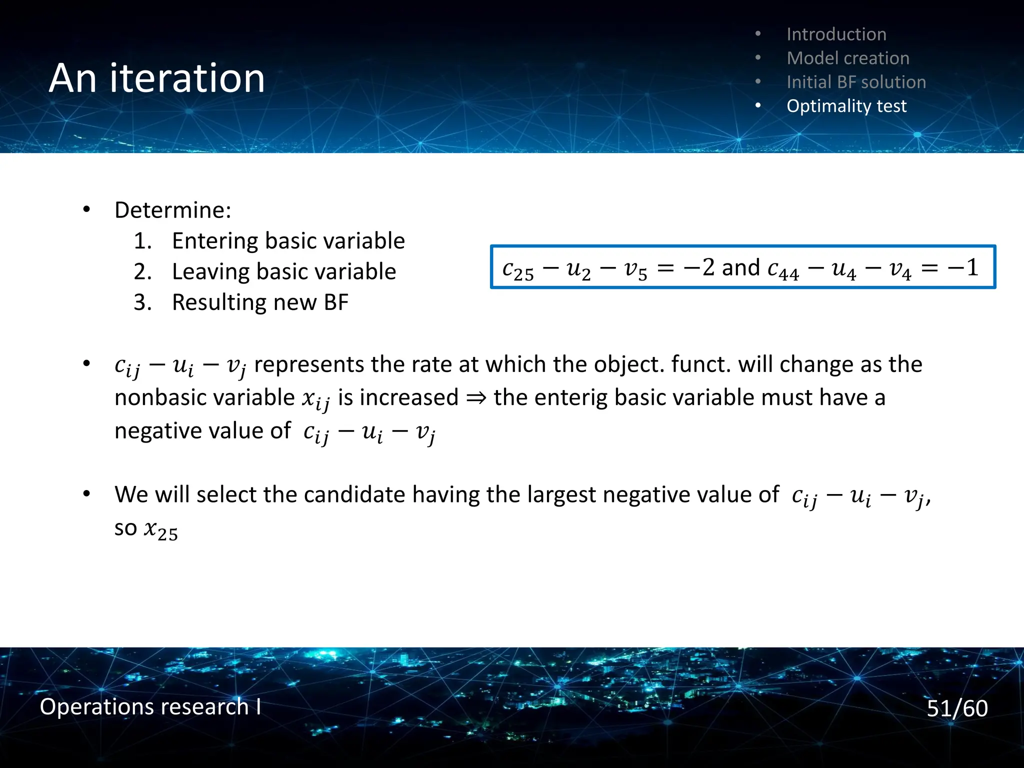
• Determine:
1. Entering basic variable
2. Leaving basic variable
3. Resulting new BF
• 𝑐𝑖𝑗 − 𝑢𝑖 − 𝑣𝑗 represents the rate at which the object. funct. will change as the
nonbasic variable 𝑥𝑖𝑗 is increased ⇒ the enterig basic variable must have a
negative value of 𝑐𝑖𝑗 − 𝑢𝑖 − 𝑣𝑗
• We will select the candidate having the largest negative value of 𝑐𝑖𝑗 − 𝑢𝑖 − 𝑣𝑗,
so 𝑥25
𝑐25 − 𝑢2 − 𝑣5 = −2 and 𝑐44 − 𝑢4 − 𝑣4 = −1
51/60
Operations research I

52. Completed initial transportation
simplex tableau
• Introduction
• Model creation
• Initial BF solution
• Optimality test
Iter. Destination
0 1 2 3 4 5 Supply 𝑢𝑖
Source
1 50 -5
2 60 -5
3 50 0
4(D) 50 -22
Demand 30 20 70 30 60 𝑍 = 2570
𝑣𝑗 19 19 18 23 22
16 16 13 22 17
14 14 13 19 15
19 19 20 23 M
M 0 M 0 0
40 10
30 30
0 20 30
50
-2
-1
+2 +2 +4
0 +1
+2 M-22
M+3 M+4
+3
52/60
Operations research I

53. Init. transportation simplex tableau
Chain reaction
• Introduction
• Model creation
• Initial BF solution
• Optimality test
Iter. Destination
0 3 4 5 Supply
Source
1 ⋯ 50
2 ⋯ 60
⋯ ⋯ ⋯ ⋯
Demand 70 30 60
13 22 17
13 19 15
40 10
30
+4
-2
+1 +
-
+
-
53/60
Operations research I

54. Init. transportation simplex tableau
Chain reaction
• Introduction
• Model creation
• Initial BF solution
• Optimality test
Iter. Destination
0 3 4 5 Supply
Source
1 ⋯ 50
2 ⋯ 60
Demand 70 30 60
13 22 17
13 19 15
40 10
30
+4
-2
+1 +
-
+
-
• Cells (2,5) and (1,3) = recipient cells (they recieve additional allocation from donor
celss)
• Cells (1,5) and (2, 3) = donor cells
54/60
Operations research I

55. Init. transportation simplex tableau
Chain reaction
• Introduction
• Model creation
• Initial BF solution
• Optimality test
Iter. Destination
0 3 4 5 Supply
Source
1 ⋯ 50
2 ⋯ 60
Demand 70 30 60
13 22 17
13 19 15
40 10
30
+4
-2
+1 +
-
+
-
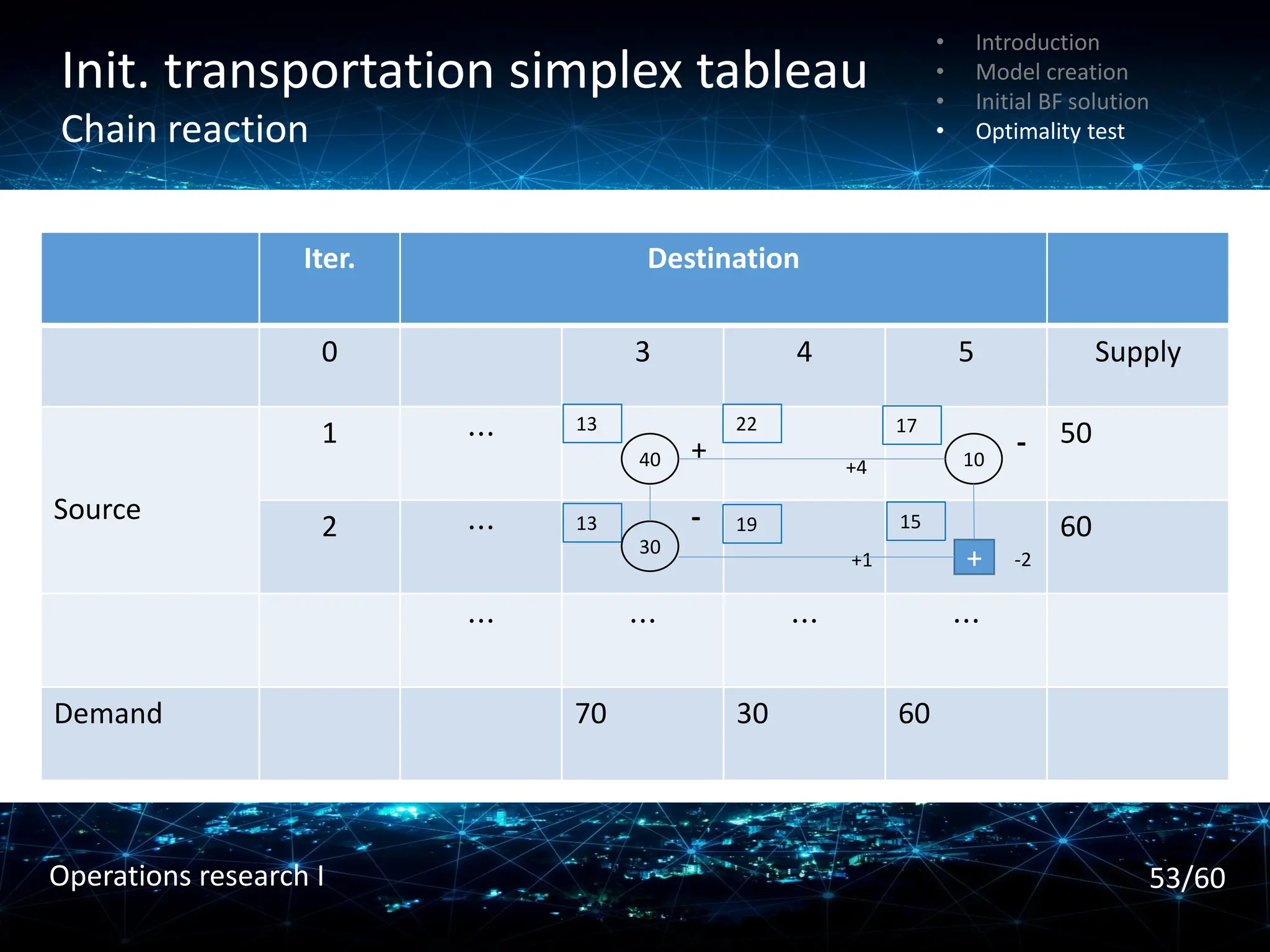
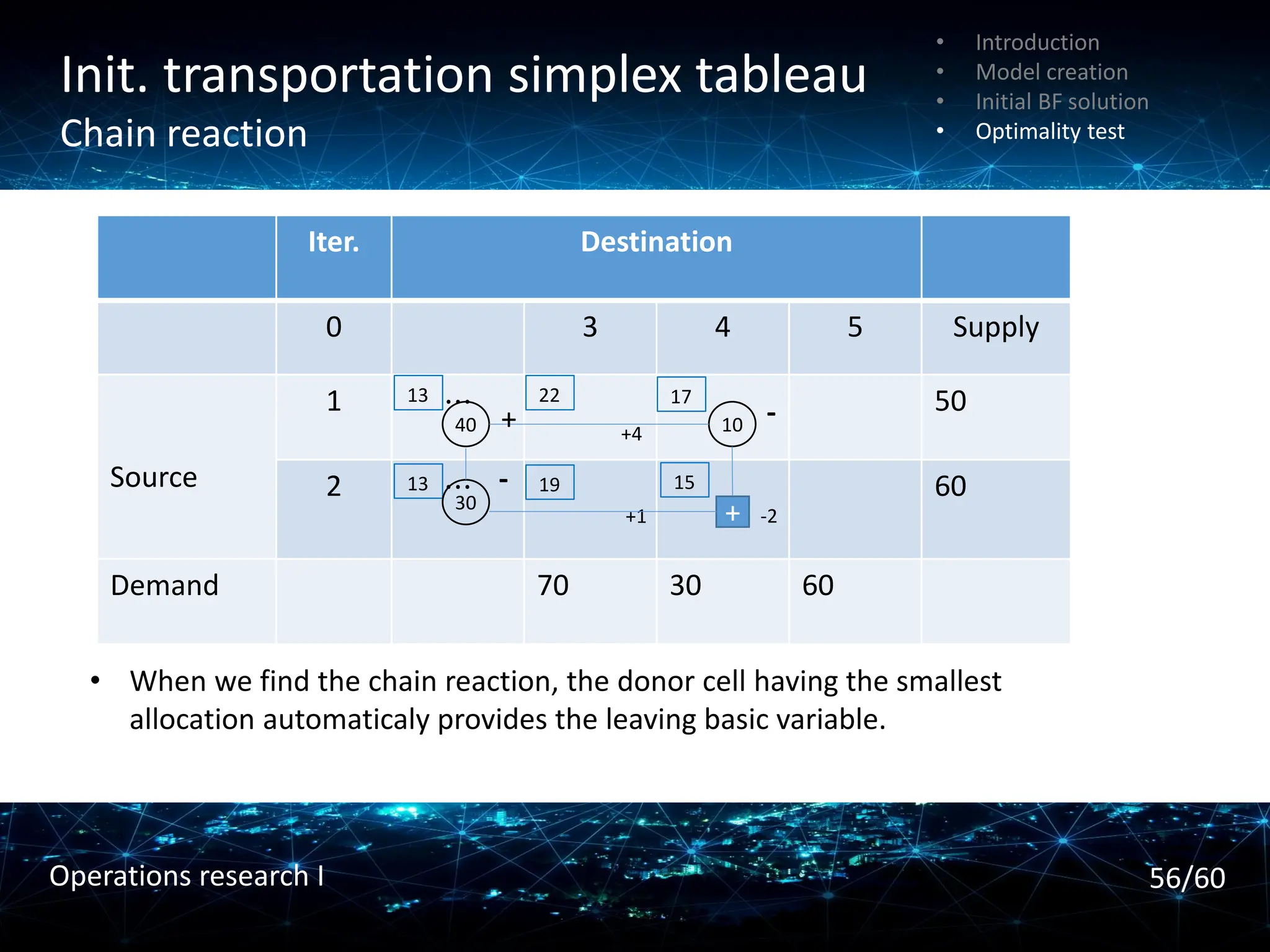
• The recipient and donor cells correspond to the basic variables in the current
BF solution
55/60
Operations research I

56. Init. transportation simplex tableau
Chain reaction
• Introduction
• Model creation
• Initial BF solution
• Optimality test
Iter. Destination
0 3 4 5 Supply
Source
1 ⋯ 50
2 ⋯ 60
Demand 70 30 60
13 22 17
13 19 15
40 10
30
+4
-2
+1 +
-
+
-
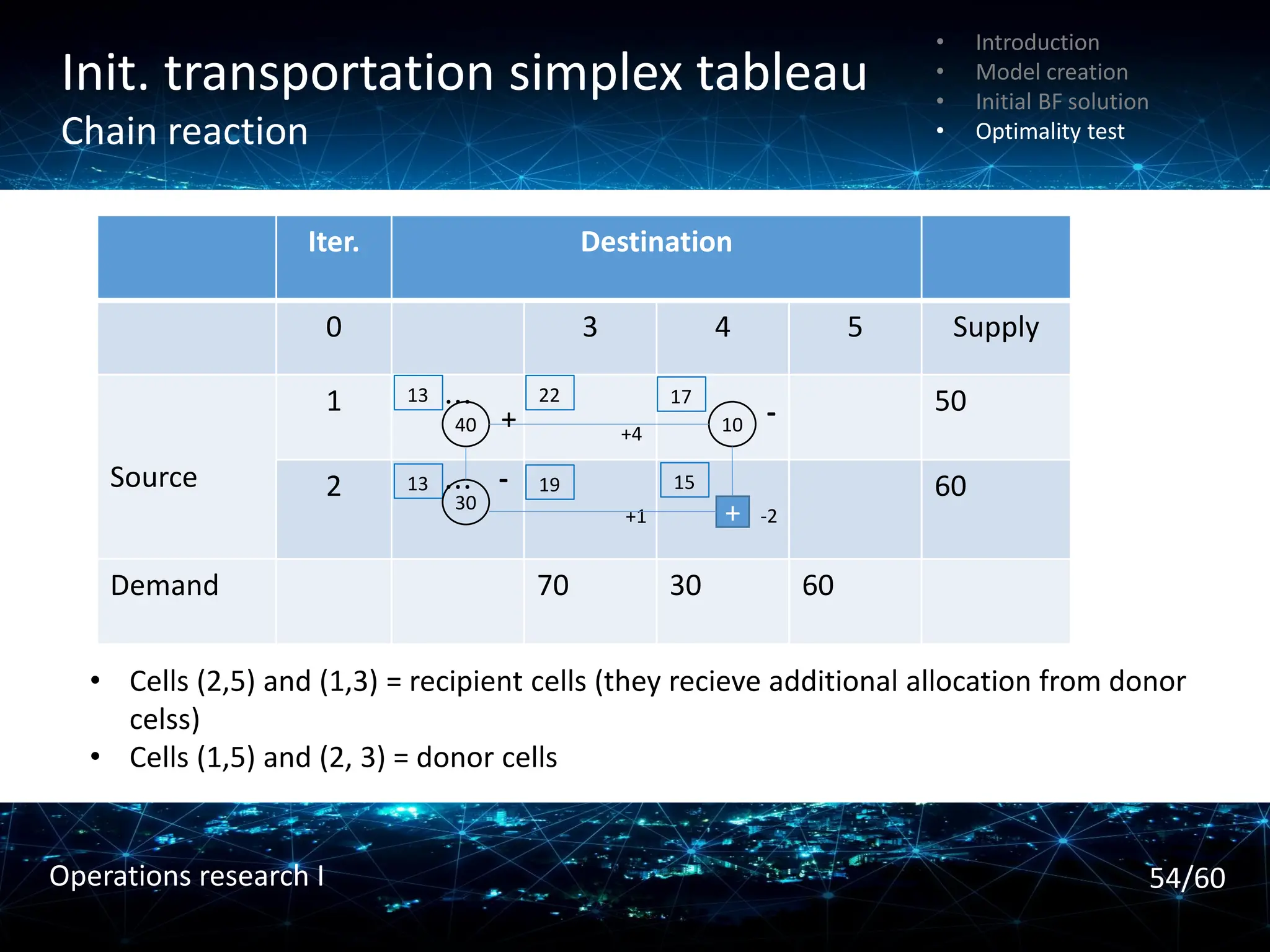
• When we find the chain reaction, the donor cell having the smallest
allocation automaticaly provides the leaving basic variable.
56/60
Operations research I

57. Init. transportation simplex tableau
New BF solution
• Introduction
• Model creation
• Initial BF solution
• Optimality test
Iter. Destination
0 3 4 5 Supply
Source
1 ⋯ 50
2 ⋯ 60
Demand 70 30 60
13 22 17
13 19 15
50
10
20
+4
-2
+1
-
+
-
• Add the value of the leaving basic variable to the allocation for each recipient
cell
• Subtract the same amount from the allocation for each donor cell
57/60
Operations research I

58. Init. transportation simplex tableau
New BF solution
• Introduction
• Model creation
• Initial BF solution
• Optimality test
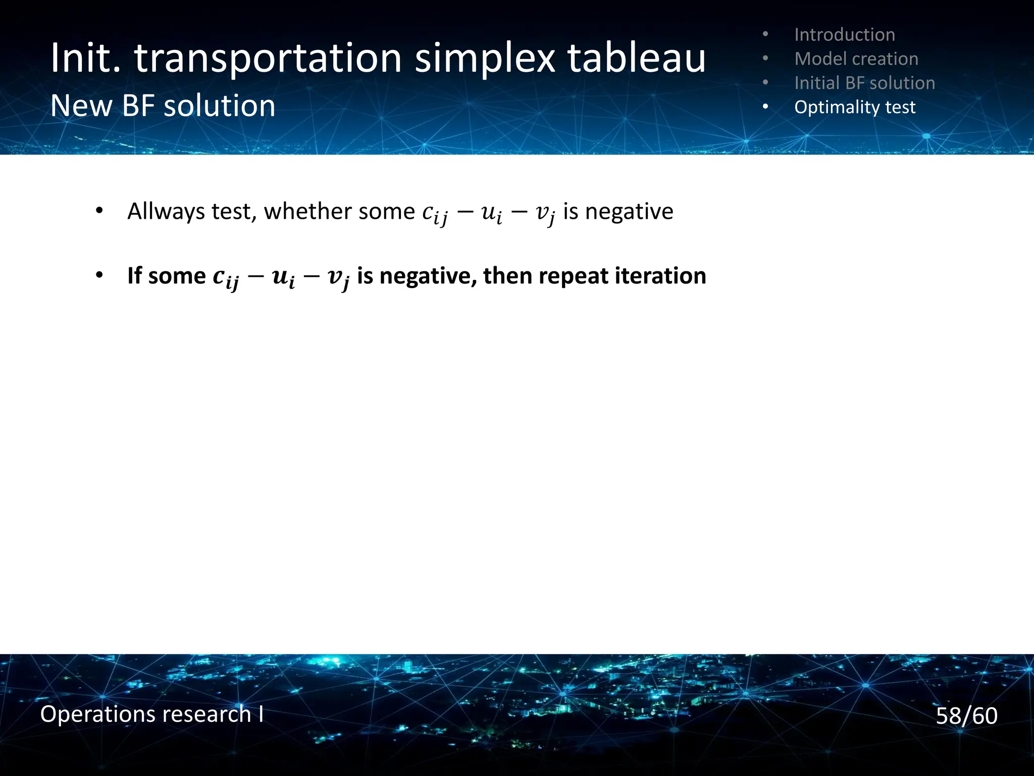
• Allways test, whether some 𝑐𝑖𝑗 − 𝑢𝑖 − 𝑣𝑗 is negative
• If some 𝒄𝒊𝒋 − 𝒖𝒊 − 𝒗𝒋 is negative, then repeat iteration
58/60
Operations research I

59. Init. transportation simplex tableau
Optimal solution
• Introduction
• Model creation
• Initial BF solution
• Optimality test
Transportation simplex tableau
Optimal solution
• Introduction
• Model creation
• Initial BF solution
• Optimality test
Iter. Destination
0 1 2 3 4 5 Supply 𝑢𝑖
Source
1 50 -7
2 60 -7
3 50 0
4(D) 50 -22
Demand 30 20 70 30 60 𝑍 = 2460
𝑣𝑗 19 19 20 22 22
16 16 13 22 17
14 14 13 19 15
19 19 20 23 M
M 0 M 0 0
50
20
30 20
20
+4 +4 +7
+2 +4
M-22
M+3 M+2
+3
+2
+2
40
0
+1
30
59/60
Operations research I

60. Init. transportation simplex tableau
Optimal solution
• Introduction
• Model creation
• Initial BF solution
• Optimality test
Transportation simplex tableau
Optimal solution
• Introduction
• Model creation
• Initial BF solution
• Optimality test
Iter. Destination
0 1 2 3 4 5 Supply 𝑢𝑖
Source
1 50 -7
2 60 -7
3 50 0
4(D) 50 -22
Demand 30 20 70 30 60 𝑍 = 2460
𝑣𝑗 19 19 20 22 22
16 16 13 22 17
14 14 13 19 15
19 19 20 23 M
M 0 M 0 0
50
20
30 20
20
+4 +4 +7
+2 +4
M-22
M+3 M+2
+3
+2
+2
40
0
+1
30
60/60
Operations research I

61. Init. transportation simplex tableau
Optimal solution
• Introduction
• Model creation
• Initial BF solution
• Optimality test
Literature
• Introduction
• Model creation
• Initial BF solution
• Optimality test
60/60
Operations research I
[1] Literature: Hillier and Lieberman: Introduction to Operations Research, 8th edition,
2005