Chapter 4R Part II

 ISDS 2001 - Matt Levy
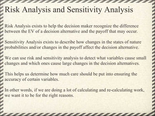
Risk Analysis and Sensitivity Analysis
Risk Analysis exists to help the decision maker recognize the difference
between the EV of a decision alternative and the payoff that may occur.

Sensitivity Analysis exists to describe how changes in the states of nature
probabilities and/or changes in the payoff affect the decision alternative.

We can use risk and sensitivity analysis to detect what variables cause small
changes and which ones cause large changes in the decision alternatives.

This helps us determine how much care should be put into ensuring the
accuracy of certain variables.

In other words, if we are doing a lot of calculating and re-calculating work,
we want it to be for the right reasons.
Risk Analysis and Sensitivity Analysis
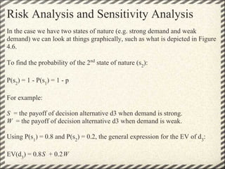
In the case we have two states of nature (e.g. strong demand and weak
demand) we can look at things graphically, such as what is depicted in Figure
4.6.

To find the probability of the 2nd state of nature (s2):

P(s2) = 1 - P(s1) = 1 - p

For example:

S = the payoff of decision alternative d3 when demand is strong.
W = the payoff of decision alternative d3 when demand is weak.

Using P(s1) = 0.8 and P(s2) = 0.2, the general expression for the EV of d3:

EV(d3) = 0.8S + 0.2W
Decision Analysis with Sample
Information
Most of the time decision makers have some notion of prior
probability.

But to make the best decision, we normally want to go out and collect
sample information about the states of nature.

From our sample information we get new sample probabilities that we
may use to revise or update prior probabilities.

These new probabilities are called posterior probabilities.

With new information we can build Influence Diagrams and Decision
Trees (see Figures 4.7 and 4.8).
Decision Strategy

A sequence of decision and chance outcomes based on yet to be
determined outcomes of chance events.

We can build this using a backward pass through a decision tree.

  - At chance nodes compute the EV by multiplying the payoff at the
end of each branch by the corresponding branch probabilities.

  - At decision nodes, select the decision branch that leads to the best
EV. This EV becomes the EV at the decision node.
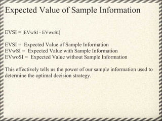
Expected Value of Sample Information

EVSI = |EVwSI - EVwoSI|

EVSI = Expected Value of Sample Information
EVwSI = Expected Value with Sample Information
EVwoSI = Expected Value without Sample Information

This effectively tells us the power of our sample information used to
determine the optimal decision strategy.
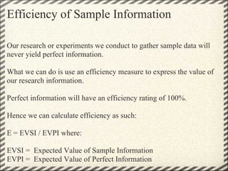
Efficiency of Sample Information

Our research or experiments we conduct to gather sample data will
never yield perfect information.

What we can do is use an efficiency measure to express the value of
our research information.

Perfect information will have an efficiency rating of 100%.

Hence we can calculate efficiency as such:

E = EVSI / EVPI where:

EVSI = Expected Value of Sample Information
EVPI = Expected Value of Perfect Information
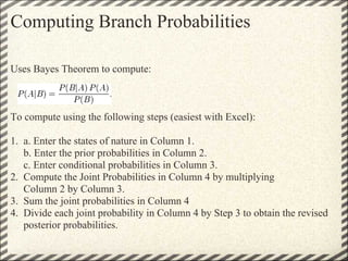
Computing Branch Probabilities

Uses Bayes Theorem to compute:


To compute using the following steps (easiest with Excel):

1. a. Enter the states of nature in Column 1.
   b. Enter the prior probabilities in Column 2.
   c. Enter conditional probabilities in Column 3.
2. Compute the Joint Probabilities in Column 4 by multiplying
   Column 2 by Column 3.
3. Sum the joint probabilities in Column 4
4. Divide each joint probability in Column 4 by Step 3 to obtain the revised
   posterior probabilities.
The End

 Read the Chapter.
 This section will be on Exam 3.
 I apologize for the work over Spring Break :-)

Chapter 4R Part II

  • 1.
    Chapter 4R PartII ISDS 2001 - Matt Levy
  • 2.
    Risk Analysis andSensitivity Analysis Risk Analysis exists to help the decision maker recognize the difference between the EV of a decision alternative and the payoff that may occur. Sensitivity Analysis exists to describe how changes in the states of nature probabilities and/or changes in the payoff affect the decision alternative. We can use risk and sensitivity analysis to detect what variables cause small changes and which ones cause large changes in the decision alternatives. This helps us determine how much care should be put into ensuring the accuracy of certain variables. In other words, if we are doing a lot of calculating and re-calculating work, we want it to be for the right reasons.
  • 3.
    Risk Analysis andSensitivity Analysis In the case we have two states of nature (e.g. strong demand and weak demand) we can look at things graphically, such as what is depicted in Figure 4.6. To find the probability of the 2nd state of nature (s2): P(s2) = 1 - P(s1) = 1 - p For example: S = the payoff of decision alternative d3 when demand is strong. W = the payoff of decision alternative d3 when demand is weak. Using P(s1) = 0.8 and P(s2) = 0.2, the general expression for the EV of d3: EV(d3) = 0.8S + 0.2W
  • 4.
    Decision Analysis withSample Information Most of the time decision makers have some notion of prior probability. But to make the best decision, we normally want to go out and collect sample information about the states of nature. From our sample information we get new sample probabilities that we may use to revise or update prior probabilities. These new probabilities are called posterior probabilities. With new information we can build Influence Diagrams and Decision Trees (see Figures 4.7 and 4.8).
  • 5.
    Decision Strategy A sequenceof decision and chance outcomes based on yet to be determined outcomes of chance events. We can build this using a backward pass through a decision tree. - At chance nodes compute the EV by multiplying the payoff at the end of each branch by the corresponding branch probabilities. - At decision nodes, select the decision branch that leads to the best EV. This EV becomes the EV at the decision node.
  • 6.
    Expected Value ofSample Information EVSI = |EVwSI - EVwoSI| EVSI = Expected Value of Sample Information EVwSI = Expected Value with Sample Information EVwoSI = Expected Value without Sample Information This effectively tells us the power of our sample information used to determine the optimal decision strategy.
  • 7.
    Efficiency of SampleInformation Our research or experiments we conduct to gather sample data will never yield perfect information. What we can do is use an efficiency measure to express the value of our research information. Perfect information will have an efficiency rating of 100%. Hence we can calculate efficiency as such: E = EVSI / EVPI where: EVSI = Expected Value of Sample Information EVPI = Expected Value of Perfect Information
  • 8.
    Computing Branch Probabilities UsesBayes Theorem to compute: To compute using the following steps (easiest with Excel): 1. a. Enter the states of nature in Column 1. b. Enter the prior probabilities in Column 2. c. Enter conditional probabilities in Column 3. 2. Compute the Joint Probabilities in Column 4 by multiplying Column 2 by Column 3. 3. Sum the joint probabilities in Column 4 4. Divide each joint probability in Column 4 by Step 3 to obtain the revised posterior probabilities.
  • 9.
    The End Readthe Chapter. This section will be on Exam 3. I apologize for the work over Spring Break :-)