The document discusses decision analysis and presents a case study on the Goferbroke Company. Goferbroke must decide whether to drill for oil or sell land with a 25% chance of containing oil. Drilling costs $100,000 but may yield $800,000 profit if successful. Selling now offers $90,000. Additional seismic analysis could update probabilities at a $30,000 cost. The final decision tree weighs expected payoffs of drilling versus selling under both scenarios of conducting or not conducting the seismic analysis.

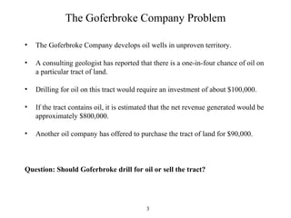
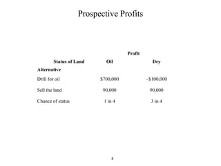
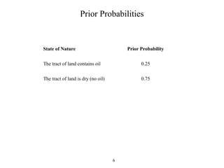
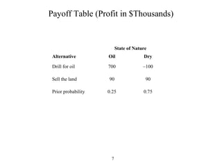
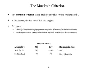
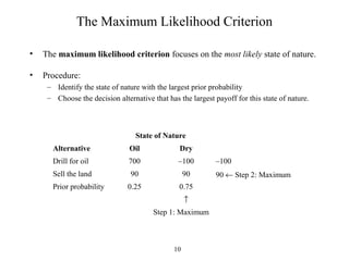
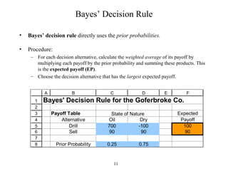
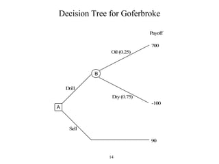
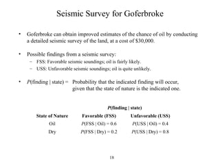
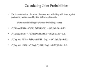
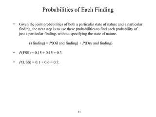
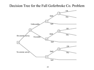
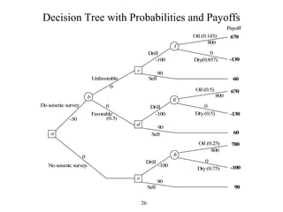
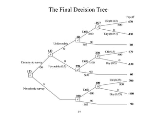
1. 1
Decision Analysis
Prof. Chandana Perera

2. 2
Decision Analysis
• Managers often must make decisions in environments that are fraught with
uncertainty.
• Some Examples
– A government contractor bidding on a new contract.
• What will be the actual costs of the project?
• Which other companies might be bidding?
• What are their likely bids?
– An agricultural firm selecting the mix of crops and livestock for the season.
• What will be the weather conditions?
• Where are prices headed?
• What will costs be?
– An oil company deciding whether to drill for oil in a particular location.
• How likely is there to be oil in that location?
• How much?
• How deep will they need to drill?
• Should geologists investigate the site further before drilling?

3. 3
The Goferbroke Company Problem
• The Goferbroke Company develops oil wells in unproven territory.
• A consulting geologist has reported that there is a one-in-four chance of oil on
a particular tract of land.
• Drilling for oil on this tract would require an investment of about $100,000.
• If the tract contains oil, it is estimated that the net revenue generated would be
approximately $800,000.
• Another oil company has offered to purchase the tract of land for $90,000.
Question: Should Goferbroke drill for oil or sell the tract?

4. 4
Prospective Profits
Profit
Status of Land Oil Dry
Alternative
Drill for oil $700,000 –$100,000
Sell the land 90,000 90,000
Chance of status 1 in 4 3 in 4

5. 5
Decision Analysis Terminology
• The decision maker is the individual or group responsible for making the
decision.
• The alternatives are the options for the decision to be made.
• The outcome is affected by random factors outside the control of the decision
maker. These random factors determine the situation that will be found when
the decision is executed. Each of these possible situations is referred to as a
possible state of nature.
• The decision maker generally will have some information about the relative
likelihood of the possible states of nature. These are referred to as the prior
probabilities.
• Each combination of a decision alternative and a state of nature results in
some outcome. The payoff is a quantitative measure of the value to the
decision maker of the outcome. It is often the monetary value.

6. 6
Prior Probabilities
State of Nature Prior Probability
The tract of land contains oil 0.25
The tract of land is dry (no oil) 0.75

7. 7
Payoff Table (Profit in $Thousands)
State of Nature
Alternative Oil Dry
Drill for oil 700 –100
Sell the land 90 90
Prior probability 0.25 0.75

8. 8
The Maximax Criterion
• The maximax criterion is the decision criterion for the eternal optimist.
• It focuses only on the best that can happen.
• Procedure:
– Identify the maximum payoff from any state of nature for each alternative.
– Find the maximum of these maximum payoffs and choose this alternative.
State of Nature
Alternative Oil Dry Maximum in Row
Drill for oil 700 –100 700 ← Maximax
Sell the land 90 90 90

9. 9
The Maximin Criterion
• The maximin criterion is the decision criterion for the total pessimist.
• It focuses only on the worst that can happen.
• Procedure:
– Identify the minimum payoff from any state of nature for each alternative.
– Find the maximum of these minimum payoffs and choose this alternative.
State of Nature
Alternative Oil Dry Minimum in Row
Drill for oil 700 –100 –100
Sell the land 90 90 90 ← Maximin

10. 10
The Maximum Likelihood Criterion
• The maximum likelihood criterion focuses on the most likely state of nature.
• Procedure:
– Identify the state of nature with the largest prior probability
– Choose the decision alternative that has the largest payoff for this state of nature.
State of Nature
Alternative Oil Dry
Drill for oil 700 –100 –100
Sell the land 90 90 90 ← Step 2: Maximum
Prior probability 0.25 0.75
↑
Step 1: Maximum

11. 11
Bayes’ Decision Rule
• Bayes’ decision rule directly uses the prior probabilities.
• Procedure:
– For each decision alternative, calculate the weighted average of its payoff by
multiplying each payoff by the prior probability and summing these products. This
is the expected payoff (EP).
– Choose the decision alternative that has the largest expected payoff.
1
2
3
4
5
6
7
8
A B C D E F
Bayes' Decision Rule for the Goferbroke Co.
Payoff Table Expected
Alternative Oil Dry Payoff
Drill 700 -100 100
Sell 90 90 90
Prior Probability 0.25 0.75
State of Nature

12. 12
Bayes’ Decision Rule
• Features of Bayes’ Decision Rule
– It accounts for all the states of nature and their probabilities.
– The expected payoff can be interpreted as what the average payoff would become if
the same situation were repeated many times. Therefore, on average, repeatedly
applying Bayes’ decision rule to make decisions will lead to larger payoffs in the
long run than any other criterion.
• Criticisms of Bayes’ Decision Rule
– There usually is considerable uncertainty involved in assigning values to the prior
probabilities.
– Prior probabilities inherently are at least largely subjective in nature, whereas sound
decision making should be based on objective data and procedures.
– It ignores typical aversion to risk. By focusing on average outcomes, expected
(monetary) payoffs ignore the effect that the amount of variability in the possible
outcomes should have on decision making.

13. 13
Decision Trees
• A decision tree can apply Bayes’ decision rule while displaying and
analyzing the problem graphically.
• A decision tree consists of nodes and branches.
– A decision node, represented by a square, indicates a decision to be made. The
branches represent the possible decisions.
– An event node, represented by a circle, indicates a random event. The branches
represent the possible outcomes of the random event.

14. 14
Decision Tree for Goferbroke
A
B
Payoff
-100
90
700
Oil (0.25)
Dry (0.75)
Drill
Sell

15. 15
Checking Whether to Obtain More Information
• Might it be worthwhile to spend money for more information to obtain better
estimates?
• A quick way to check is to pretend that it is possible to actually determine the true
state of nature (“perfect information”).
• EP (with perfect information) = Expected payoff if the decision could be made
after learning the true state of nature.
• EP (without perfect information) = Expected payoff from applying Bayes’
decision rule with the original prior probabilities.
• The expected value of perfect information is then
EVPI = EP (with perfect information) – EP (without perfect information).

16. 16
Expected Payoff with Perfect Information
3
4
5
6
7
8
9
10
11
B C D
Payoff Table
Alternative Oil Dry
Drill 700 -100
Sell 90 90
Maximum Payoff 700 90
Prior Probability 0.25 0.75
EP (with perfect info) 242.5
State of Nature
Value of Perfect Information = 242.5 -100

17. 17
Using New Information to Update the Probabilities
• The prior probabilities of the possible states of nature often are quite
subjective in nature. They may only be rough estimates.
• It is frequently possible to do additional testing or surveying (at some
expense) to improve these estimates. The improved estimates are called
posterior probabilities.

18. 18
Seismic Survey for Goferbroke
• Goferbroke can obtain improved estimates of the chance of oil by conducting
a detailed seismic survey of the land, at a cost of $30,000.
• Possible findings from a seismic survey:
– FSS: Favorable seismic soundings; oil is fairly likely.
– USS: Unfavorable seismic soundings; oil is quite unlikely.
• P(finding | state) = Probability that the indicated finding will occur,
given that the state of nature is the indicated one.
P(finding | state)
State of Nature Favorable (FSS) Unfavorable (USS)
Oil P(FSS | Oil) = 0.6 P(USS | Oil) = 0.4
Dry P(FSS | Dry) = 0.2 P(USS | Dry) = 0.8

19. 19
Decision Tree for the Full Goferbroke Co. Problem
a
b
c
d
e
f
g
h
Do seismic survey
No seismic survey
Unfavorable
Favorable
Drill
Sell
Drill
Sell
Oil
Dry
Oil
Dry
Oil
Dry
Sell
Drill

20. 20
Calculating Joint Probabilities
• Each combination of a state of nature and a finding will have a joint
probability determined by the following formula:
P(state and finding) = P(state) P(finding | state)
• P(Oil and FSS) = P(Oil) P(FSS | Oil) = (0.25)(0.6) = 0.15.
• P(Oil and USS) = P(Oil) P(USS | Oil) = (0.25)(0.4) = 0.1.
• P(Dry and FSS) = P(Dry) P(FSS | Dry) = (0.75)(0.2) = 0.15.
• P(Dry and USS) = P(Dry) P(USS | Dry) = (0.75)(0.8) = 0.6.

21. 21
Probabilities of Each Finding
• Given the joint probabilities of both a particular state of nature and a particular
finding, the next step is to use these probabilities to find each probability of
just a particular finding, without specifying the state of nature.
P(finding) = P(Oil and finding) + P(Dry and finding)
• P(FSS) = 0.15 + 0.15 = 0.3.
• P(USS) = 0.1 + 0.6 = 0.7.

22. 22
Calculating the Posterior Probabilities
• The posterior probabilities give the probability of a particular state of nature,
given a particular finding from the seismic survey.
P(state | finding) = P(state and finding) / P(finding)
• P(Oil | FSS) = 0.15 / 0.3 = 0.5.
• P(Oil | USS) = 0.1 / 0.7 = 0.14.
• P(Dry | FSS) = 0.15 / 0.3 = 0.5.
• P(Dry | USS) = 0.6 / 0.7 = 0.86.

23. 23
Probability Tree Diagram
0.25(0.6) = 0.15
Oil and FSS Oil, given FSS
0.25(0.4) = 0.1
Oil and USS
0.75(0.2) = 0.15
0.75(0.8) = 0.6
Dry and USS
Dry and FSS
Dry, given USS
Dry, given FSS
Oil, given USS
= 0.50.15
0.3
0.1
0.7
= 0.14
0.15
0.3
= 0.5
0.6
0.7
= 0.86
Prior
Probabilities
P(state)
Conditional
Probabilities
P(finding | state)
Joint
Probabilities
P(state and finding)
Posterior
Probabilities
P(state | finding)
Unconditional probabilities: P(FSS) = 0.15 + 0.15 = 0.3
P(finding) P(USS) = 0.1 + 0.6 = 0.7
0.6
FSS, given Oil
0.4
USS, given Oil
0.2
FSS, given Dry
0.8
USS, given Dry
0.25
Oil
0.75
Dry

24. 24
Posterior Probabilities
P(state | finding)
Finding Oil Dry
Favorable (FSS) P(Oil | FSS) = 1/2 P(Dry | FSS) = 1/2
Unfavorable (USS) P(Oil | USS) = 1/7 P(Dry | USS) = 6/7

25. 25
Decision Tree for the Full Goferbroke Co. Problem
a
b
c
d
e
f
g
h
Do seismic survey
No seismic survey
Unfavorable
Favorable
Drill
Sell
Drill
Sell
Oil
Dry
Oil
Dry
Oil
Dry
Sell
Drill

26. 26
Decision Tree with Probabilities and Payoffs
a
b
c
d
e
f
g
h
Payoff
670
-130
60
670
-130
60
700
-100
90
Doseismic survey
Noseismic survey
Unfavorable
Favorable
Drill
-100
90
Sell
Drill
-100
90
Sell
Drill
-100
90
Sell
Oil (0.143)
800
0
Dry(0.857)
Oil (0.5)
800
0
Dry(0.5)
Oil (0.25)
800
Dry(0.75)
0
(0.3)-30
0
0
0

27. 27
The Final Decision Tree
a
b
c
d
e
f
g
h
Payoff
670
-130
60
670
-130
60
700
-100
90
100
270
60
123
123
-15.7
270
100
Doseismic survey
Noseismic survey
-30
0
Unfavorable
0
0
Favorable (0.3)
Drill
-100
90
Sell
Drill
-100
90
Sell
Drill
-100
90
Sell
Oil (0.143)
800
0
Dry(0.857)
Oil (0.5)
800
0
Dry(0.5)
Oil (0.25)
800
0
Dry(0.75)