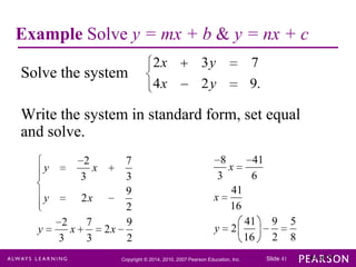
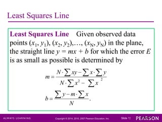
This section discusses finding the intersection point of two lines. To find the intersection of lines in the form y=mx+b and y=nx+c:
1. Set the two equations equal to each other and solve for x
2. Substitute the x value into one equation and solve for y
This will give the point where the two lines intersect. An example finds the intersection of the lines 2x-3y=7 and 4x-2y=5 by setting the equations equal and solving the resulting equation for x and y.


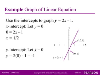
![Graph of y = mx + b
To graph the equation y = mx + b:
1. Plot the y-intercept (0,b).
2. Plot some other point. [The most convenient
choice is often the x-intercept.]
3. Draw a line through the two points.
Copyright © 2014, 2010, 2007 Pearson Education, Inc.
Slide 17
17 of 71](https://image.slidesharecdn.com/chapter1-linearequationsandstraightlines-131125171307-phpapp02/85/Chapter-1-linear-equations-and-straight-lines-17-320.jpg)