Chapter 0 credit neural network

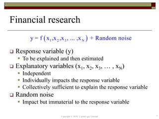
Credit Neural Network
with Neural Designer
This presentation file is prepared in accordance with
the text book
“Credit Neural Network with Neural Designer”
Website : https://sites.google.com/site/quanrisk
E-mail : quanrisk@gmail.com
Copyright © 2019 CapitaLogic Limited

Declaration
 Copyright © 2019 CapitaLogic Limited.
 All rights reserved. No part of this presentation file may be
reproduced, in any form or by any means, without written
permission from CapitaLogic Limited.
 Authored by Dr. LAM Yat-fai (林日辉),
Director, CapitaLogic Limited,
Adjunct Professor of Finance, City University of Hong Kong,
Doctor of Business Administration,
CFA, CAIA, CAMS, FRM, PRM.
2Copyright © 2019 CapitaLogic Limited

Outline
 Data preparation
 Classical regressions
 Monotonic neural network
 Continuous response network
 Credit neural network
 Shadow credit rating
 LGD of residential mortgages

What is research?
 There is a result
 Theory
 Which factors cause this result?
 How increases and/or decreases in these factors
impact the result?
 Testing
 Does the theory work in real life scenarios?

Financial research
 Response variable (y)
 To be explained and then estimated
 Explanatory variables (x1, x2, x3, … , xN)
 Independent
 Individually impacts the response variable
 Collectively sufficient to explain the response variable
 Random noise
 Impact but immaterial to the response variable
 1 2 3 Ny = f x ,x ,x , ... ,x + Random noise

Data preparation
 Outliers
 Relevancy
 Inter-dependency
 Randomization
 Consistency
 Sampling
Copyright © 2019 CapitaLogic Limited 6
Example 1.1

Outliers
 Smallest 1% value of the variables
 Largest 1% value of the variables
 To exclude outliers
Example 1.2

Relevancy
 Between the response variable and an
explanatory
 Quantified by the Spearman’s ρ
 Smaller t-statistic and larger p-value suggest
weaker relevancy
 To exclude irrelevant explanatory variables
Example 1.3

Inter-dependency
 Between any two explanatory variables
 Quantified by the Spearman’s ρ
 Larger Spearman’s ρ suggests stronger inter-
dependency between two explanatory variables
 To drop one of the inter-dependent
explanatory variables
Example 1.4

Randomization
 For a continuous response variable, order the
records randomly
 For a categorical response variable, order the
records randomly for each category of the
response variable
Example 1.5

Consistency
 Consistent variables
 Cover a similar range
 Increase in an explanatory variable
=> Increase in the response variable
while holding other explanatory variables fixed
 More effective and efficient for computer
implementation
Example 1.6

Consistent transformation
12
Consistent variable
Value of the variable - Average of the variable
=
Standard deviation of the variable
Spearman's ρ between the variable
× Sign
and the response variable
 
 
 

Inverse consistent transformation
13
Value of the variable
= Consistent variable
× Standard deviation of the variable
Spearman's ρ between the variable
× Sign
and the response variable
+ Average of the variable
 
 
 

Sampling
 For a continuous explanatory variable
 Training data set
 No. of explanatory variables × 15 or
 1% of all records, which ever is more
 0.5% of all records, which ever is more
 For each value of a categorical explanatory variable
 1% of all records, which ever is more
 0.5% of all records, which ever is more

Outline

Simple linear regression
 Explanatory variable (x)
 Sufficient to explain the response variable
 Random noise
 Linear relationship
 Increase in one unit of the explanatory variable always increases the
same level of response variable; or
 Increase in one unit of the explanatory variable always decreases the
same level of response variable
0 1y = a + a x + Random noise

Polynomial regression
 Explanatory variable (x)
 Sufficient to explain the response variable
 Random noise
 Advantage
 Increase in the order of polynomial will increase the fitness
 Disadvantage
 Increase in the order of polynomial may introduce over fitting
2 3 N
0 1 2 3 Ny = a + a x + a x + a x + ... + a x + Random noise
Example 2.1
Example 2.2

Multiple linear regression
 Independent
 Random noise
 Normally distributed with constant standard deviation
 Independent
 Linear relationship
 Holding other explanatory variables fixed
 Increase in one unit of an explanatory variable always increases the same level of response variable; or
 Increase in one unit of an explanatory variable always decreases the same level of response variable
0 1 1 2 2 3 3 N Ny = a + a x + a x + a x + ... + a x + Random noise
Example 2.3

Probit transformation
19
   
   
2
Probit
-
-1
1 τ
Probistic = exp - dτ
22π
Probistic = Φ Probit 0,1
Probit = Φ Probistic - ,+

 
 
 
 


Probistic regression
 Either 0 or 1
 Independent
 Consistent
 Random noise
 
0 1 1 2 2 3 3 N NProbit = a + a x + a x + a x + ... + a x + Random noise
Probistic = Φ Probit
y = 0 if Probistic < 50%
= 1 if Probistic 50%
Example 2.4

Probit transformation

22
Maximum likelihood method
 
   
 
0 1 1 2 2 3 3 N N
1 1 1
1 2 3
1 0 0
U 1 2
0
3
Probit = a + a x + a x + a x + ... + a x
Probistic = Φ Probit
L = Probistic × Probistic × Probistic
× × Probistic × 1 - Probistic × 1 - Probistic
× 1 - Probistic × × 1 - Probisti 
     
     
   
0
V
1 1 1
1 2 3
1 0 0
U 1 2
0 0
3 V
c
Mazimize ln(L) = ln Probistic + ln Probistic + ln Probistic
+ + ln Probistic + ln 1 - Probistic + ln 1 - Probistic
+ ln 1 - Probistic + + ln 1 - Probistic

Outline

Monotonic neural network
 To release the limitations of multiple linear
regression
WITHOUT
 Introducing complex mathematics
 An extremely simplified version of neural
network
 The entry level of artificial intelligence, machine
learning and deep learning

Requirements of
monotonic neural network
 Consistent
 To be explained and estimated
 Consistent
 Random noise
 1 2 3 Ny = f x ,x ,x , ... ,x + Random noise

Monotonic: Black Scholes model
Explanatory variable Change Call option value
Stock price
↑
↑
Strike price ↓
Volatility ↑
Risk free rate ↑
Time to maturity ↑

Monotonic: Merton’s model
Explanatory variable Change Credit quality
Value of equity
↑
↑
Value of liabilities ↓
Volatility of equity ↑

Not monotonic
x1 x2 y
+
↑
↑
- ↓
1 2y = x x + Random noise

Implementation of a neural network
 Variables from theory and/or experience
 A response variable
 A set of explanatory variables
 Prepare samples
 Training : Testing = 3 : 1
 Set up the neural network
 Train the neural network with training data set
 Calculate values with the neural network
 Assess the in sample accuracy with the training data set
 Assess the out sample accuracy with the testing data set
 Use the neural network to conduct estimation
 Assess the monotonicity with scenario analysis to verify the theory

Network structure
Explanatory
variables
Response
variable
Neurons
30
y
Example 3.1

Optimization
 For each neuron k
 Response variable
 Sum of squared error
 Find a set of as and bs to minimize the SSE
31
 
 
 
k k k k k k
0 1 1 2 2 3 3 N N
k k k N
0 1 2 3 N
2
n =Φ a + a x + a x + a x + ... + a x
y est. = Φ b + b n + b n + b n + ... + b n
SSE = y - y est.

No. of as and bs
 No. of nodes
 N explanatory variables
 N neurons
 One response variables
 Each neuron
 N + 1 as
 N + 1 bs
 Total number
 (N + 1)2
 Including irrelevant or dependent explanatory variable will
waste a lot of computing power

Advantages of
 Higher predictive power
 Minimum structural assumption
 Consistency
 Simple network structure
 Single neuron layer
 No. of neurons = No. of explanatory variables
 Moderate computing power
 Robust to irrelevant and/or dependent explanatory variables at a cost
of computing power
 Can be easily applied to most financial analysis
 Particularly suitable for marginally decreasing response variable
 For example, PD

Disadvantages of
 Rely on theory and/or experience to identify
explanatory variables
 May incorporate the effect of random noise
during training
 No straight forward mathematical formulation
 More samples

Outline

Variables and samples
 y
 Explanatory variables
 x1, x2, x3
 Sufficient no. of samples
Example 4.1

Create a neural network

Import training data
Example 4.1

Train the neural network
Example 4.2

Conduct estimation
Example 4.3

Testing
 Estimate y with the training and testing data
sets
 Compare with the historical response variable
 Calculate the error
41
y est.
Absoulte percentage error = - 1 × 100%
y

Accuracy matrix
42
% error < Count Percentage
50% 184 92%
30% 176 88%
10% 126 63%
5% 58 29%
3% 36 18%
1% 10 5%
Total 200 The larger the better

Estimation
 Given a set of explanatory variables without
response variable
 Use the neural network to estimate the ys
Example 4.4

Monotonicity analysis
 Baseline scenarios
 All explanatory variables set to
 The medians
 The averages
 The maximums
 The minimums
 While fixing other explanatory variables
 Vary one explanatory variable from the minimum to the
maximum
 Conduct estimation
 Plot response variable vs explanatory variable
 Repeat for other explanatory variables
Example 4.6

Example 4.7

Exception
 Violation of monotonicity
 The theory and/or experience need to be reviewed
 Inter-dependency among explanatory variables
 Too much random noise
 Response variable insensitive to an
explanatory variable
 The explanatory variable may be irrelevant
 Remove the explanatory and re-build the neural
network

Outline

Merton’s corporate default model
 Market’s view of credit quality can be derived
from observable
 x1 = Market value of equity
 x2 = Book value of liabilities
 x3 = Volatility of equity

Example 5.1
Example 5.2
Example 5.3

 Coded PD of the listed companies
 0 for survival and 1 for default
 x1, x2, x3

Testing
 Conduct estimation with the training and
testing data sets on the coded PD
 Use the neural network to estimate a PD
 If PD < 50%, then a bad borrower
 If PD > 50%, then a good borrower

Accuracy matrix
52
Match ? Count Percentage
Yes 180 90%
No 20 10%
Total 200
The more Yes
the better

Estimation
the coded PD
 Use the neural network to estimate the PDs
 If PD < 50%, then a bad borrower
 If PD > 50%, then a good borrower
Example 5.4

Outline

Merton’s corporate default model
 Market’s view of credit quality can be derived
from observable
 x1 = Market value of equity
 x2 = Book value of liabilities
 x3 = Volatility of equity

Example 6.1
Example 6.2
Example 6.3

Shadow credit rating
 The idea of using credit ratings from major
credit agencies to derive a relationship
between credit rating and explanatory
variables
 Assume that the credit ratings are largely
accurate

 Credit rating
 x1, x2, x3

Testing
 Estimate the probabilities of credit ratings with
the training and testing data sets
 Select the credit rating with the highest
probability
 Map the credit rating to the rank

Accuracy matrix
60
Variation Count Percentage
0 152 76%
1 42 21%
2 4 2%
3 2 1%
Total 200
The more 0 variation
the better

Estimation
credit rating
 Use the neural network to estimate the
probabilities of credit ratings
 Select the credit rating with the highest
probability
Example 6.4

Outline

LGD of collateralized lending
 Factor impacting the LGD
 Outstanding loan amount
 Current value of collateral
 Drift of collateral value
 Volatility of collateral value
 x1 = Loan to value ratio
 x2 = Drift of collateral value
 x3 = Volatility of collateral value

Example 7.1
Example 7.2
Example 7.3

 Credit rating
 x1, x2, x3

Testing
 Estimate the LGD with the training and testing
data sets

Estimation
LGD
 Use the neural network to estimate the LGDs
Example 7.4

Deep learning
 Many explanatory variables
 Many layers of neurons
 Several response variables
 Can handle very complex relationships
 Non-monotonic relationships
 Periodic relationships
 Require huge computing power

Deep learning neural network
Explanatory
variables
Response
variables
Layers of
neurons
69
y

Chapter 0 credit neural network

More Related Content

Similar to Chapter 0 credit neural network

More from crmbasel

Recently uploaded

Chapter 0 credit neural network