The document discusses power system stabilizers (PSS) and provides context for the thesis. It summarizes that the thesis will investigate modifying the input signal of a specific type of PSS and apply it to a power system to damp low frequency oscillations, without providing an exhaustive literature review. Details of the PSS structure, tuning methods, and considered input signals are given in later chapters.

1. 4
POWER SYSTEM STABILIZERS
Power system stabilizer (PSS) controller design, methods of combining the PSS with the
excitation controller (AVR), investigation of many different input signals and the vast field of
tuning methodologies are all part of the PSS topic. This thesis is an investigation into modifying
the input of a specific type of PSS as applied to a power system, and is not intended to serve as an
exhaustive review of the domain of PSS application and design. The references related to this
topic, [18-29], provide a survey of the state-of-the-art of this topic. This chapter will focus on
providing a review of a few of the technologies and approaches, with the goal of making the case
for using this type of controller to solve the low frequency inter-area oscillation problem. Details
such as the type of PSS structure selected, tuning methods for controllers with and without the
use of SPMs, and input signals considered are given in Chapter 6.
4.1 Control Action and Controller Design
The action of a PSS is to extend the angular stability limits of a power system by providing
supplemental damping to the oscillation of synchronous machine rotors through the generator
excitation. This damping is provided by a electric torque applied to the rotor that is in phase with
the speed variation. Once the oscillations are damped, the thermal limit of the tie-lines in the
system may then be approached. This supplementary control is very beneficial during line outages
and large power transfers [23,24]. However, power system instabilities can arise in certain
circumstances due to negative damping effects of the PSS on the rotor. The reason for this is that
PSSs are tuned around a steady-state operating point; their damping effect is only valid for small
excursions around this operating point. During severe disturbances, a PSS may actually cause the
generator under its control to lose synchronism in an attempt to control its excitation field [24].
Input 1 + sT1 1 + sT3 sK STW VPSS
1 + sT2 1 + sT4 1 + sTW
Figure 4.1: Lead-Lag Power System Stabilizer [23]
21

2. A “lead-lag” PSS structure is shown in Figure 4.1. The output signal of any PSS is a voltage
signal, noted here as VPSS(s), and added as an input signal to the AVR/exciter. For the structure
shown in Figure 4.1, this is given by
sK S TW (1 + sT1 ) (1 + sT3 )
VPSS(s) = Input(s ) (4.1)
(1 + sTW ) (1 + sT2 ) (1 + sT4 )
This particular controller structure contains a washout block, sTW/(1+sTW), used to reduce the
over-response of the damping during severe events. Since the PSS must produce a component of
electrical torque in phase with the speed deviation, phase lead blocks circuits are used to
compensate for the lag (hence, “lead-lag’) between the PSS output and the control action, the
electrical torque. The number of lead-lag blocks needed depends on the particular system and the
tuning of the PSS. The PSS gain KS is an important factor as the damping provided by the PSS
increases in proportion to an increase in the gain up to a certain critical gain value, after which the
damping begins to decrease. All of the variables of the PSS must be determined for each type of
generator separately because of the dependence on the machine parameters. The power system
dynamics also influence the PSS values. The determination of these values is performed by many
different types of tuning methodologies, as will be shown in Section 4.3.
Other controller designs do exist, such as the “desensitized 4-loop” integrated AVR/PSS
controller used by Electricité de France [26] and a recently investigated proportional-integral-
derivative (PID) PSS design [27]. Differences in these two designs lie in their respective tuning
approaches for the AVR/PSS ensemble; however, the performance of both structures is similar to
those using the lead-lag structure.
4.2 Input Signals
The input signal for the PSSs in the system is also a point of debate. The signals that have been
identified as valuable include deviations in the rotor speed (∆ω = ωmach - ωo), the frequency (∆f),
the electrical power (∆Pe) and the accelerating power (∆Pa). Since the main action of the PSS is
to control the rotor oscillations, the input signal of rotor speed has been the most frequently
advocated in the literature [1,11]. Controllers based on speed deviation would ideally use a
differential-type of regulation and a high gain. Since this is impractical in reality, the previously
mentioned lead-lag structure is commonly used. However, one of the limitations of the speed-
input PSS is that it may excite torsional oscillatory modes [11,23].
A power/speed (∆Pe-ω, or delta-P-omega) PSS design was proposed as a solution to the torsional
interaction problem suffered by the speed-input PSS [25]. The power signal used is the generator
electrical power, which has high torsional attenuation. Due to this, the gain of the PSS may be
increased without the resultant loss of stability, which leads to greater oscillation damping [11].
A frequency-input controller has been investigated as well. However, it has been found that
frequency is highly sensitive to the strength of the transmission system - that is, more sensitive
when the system is weaker - which may offset the controller action on the electrical torque of the
22

3. machine [23]. Other limitations include the presence of sudden phase shifts following rapid
transients and large signal noise induced by industrial loads [11]. On the other hand, the
frequency signal is more sensitive to inter-area oscillations than the speed signal, and may
contribute to better oscillation attenuation [23-25].
The use of a power signal as input, either the electrical power (∆Pe) or the accelerating power
(∆Pa = Pmech - Pelec), has also been considered due to its low level of torsional interaction. The
∆Pa signal is one of the two involved in the “4-loop” AVR/PSS controller from [26], even though
the tuning method related to this design approach is valid for other input signals.
4.3 Control and Tuning
The conflicting requirements of local and inter-area mode damping and stability under both small-
signal and transient conditions have led to many different approaches for the control and tuning of
PSSs. Methods investigated for the control and tuning include state-space/frequency domain
techniques [19,20], residue compensation [22], phase compensation/root locus of a lead-lag
controller [23-25], desensitization of a robust controller [26], pole-placement for a PID-type
controller [27], sparsity techniques for a lead-lag controller [28] and a strict linearization
technique for a linear quadratic controller [29]. The diversity of the approaches can be accounted
for by the difficulty of satisfying the conflicting design goals, and each method having its own
advantages and disadvantages. This is the crux of the problem of low frequency oscillation
damping by the application of power system stabilizers.
This thesis is not intended to provide a qualitative analysis of each of these techniques; rather, the
improvement of the oscillation damping and resulting stability improvement of an existing PSS
design through the use of synchronized phasor measurements is the final goal. Through the
analysis performed here, it will be shown that the use of synchronized phasor measurements can
improve the damping of an inter-area mode beyond that of an “optimally” tuned PSS. It will also
be shown that the local and inter-area modes are effectively decoupled, without a loss of stability
of either mode.
23

4. 5
POWER SYSTEM MODELING
This chapter presents the models used for the generator, turbine and speed governor, automatic
voltage regulators and power system stabilizers followed by a detailed description of the two-
area, 4-machine test power system.
5.1 Generator Model
There are several models which have been used in modeling synchronous machines for stability
studies, some including damper windings and transient flux linkages, some neglecting them. A
two-axis model that includes one damper winding in the d-axis (direct axis) and two in the q-axis
(quadrature axis) along with the transient and sub-transient characteristics of the machine is used
in EUROSTAG [30,31,32], the software package used in part for this research. This model will
be discussed here and involves the transformation of the machine variables to a common rotor-
based reference frame through the Park’s transformation [11,30,33]. This transformation changes
a reference frame fixed with the stator to a rotating reference frame fixed with respect to the
rotor, namely the direct axis (d-axis), the quadrature axis (q-axis) and a third axis associated with
the zero sequence component current (0-axis). Eventually, the latter is dropped from the model
due the fact that the zero sequence current is equal to zero for a balanced system.
The dq-axis model includes the transient and sub-transient characteristics of the machine. The
latter are governed by
&
u d = − ra i d + ωλ q − λ d (5.1)
&
u q = − ra i q + ωλ d − λ q (5.2)
&
u f = rf i f + λ f (5.3)
&
0 = rD i D + λ D (5.4)
&
0 = rQ1i Q1 + λ Q1 (5.5)
&
0 = rQ2 i Q2 + λ Q2 (5.6)
24

5. The common flux terms are
λ AD = M d (i d + i f + i D ) (5.7)
(
λ AQ = M q i q + i Q1 + i Q2 ) (5.8)
Once the non-state d- and q-axis variables have been eliminated, these equations will encompass
four state variables per machine. The final two state equations are provided by the rotor swing
equation in first order, ODE form:
2Hω = TM − TE = TM − λ q i d − λ d i q
& (5.9)
&
Θ = ω oω (5.10)
These equations represent the x = f ( x, u) model of the system. The final form of these state
&
equations is given after the linearization is performed in Section 5.5. The variable definitions for
(5.1) - (5.10) are summarized in Table 5.1.
Variable Units Definitions
xd, xq pu d- and q-axes synchronous reactances
x’d, x’q pu d- and q-axes transient reactances
x’’d, x’’q pu d- and q-axes sub-transient reactances
Ra pu stator resistance
Xl pu stator leakage inductance
T’do, T’qo sec d- and q-axes transient open circuit time constant
T’’do, T’’qo sec d- and q-axes sub-transient open circuit time constant
H pu sec stored energy at rated speed, inertia constant
ud, uq, uf pu d-axis, q-axis terminal and field winding voltages
id, iq, if pu d-axis, q-axis armature and field winding currents
iD, iQ1, iQ2 pu d- and q-axes damper winding currents
lD,lf pu d-axis damper and field winding fluxes
lQ1, lQ2 pu q-axis damper winding fluxes
rD,rf pu d-axis damper and field winding resistances
rQ1,rQ2 pu q-axis damper winding resistances
lAD, lAQ pu d- and q-axes mutual fluxes
Md, Mq pu d- and q-axes mutual inductances
TE Nm electrical torque
TM Nm mechanical torque
Θ rad generator rotor angle
ω rad/sec generator rotor angle speed
ωo rad/sec rated generator rotor angle speed
Table 5.1: Generator Model Variable Definitions
5.2 Speed Governor Model
To provide the mechanical torque and mechanical power variables during the dynamic
simulations, the turbine/speed governor model shown in Figure 5.1 was used [34]. The model
25

6. comprises a single simple-lag block, two lead-lag blocks and an input torque limiter. Based on
this diagram, the equations that describe the turbine/speed-governor for each machine are given
by
Tm = Pm/ω (5.11)
T & 1
Pm = 4 A 4 + ( A 4 − Pm )
& (5.12)
T5 T5
T & 1
A 4 = 3 A 2 + (A 2 − A 4 )
& (5.13)
TC TC
1
A 2 = (TMin − A 2 )
& (5.14)
TS
TMAX if TMI ≥ TMAX

TMin =  TMIN if TMAX > TMI > 0 (5.15)
 0 TMI ≤ 0
 if
TMI = K(1- ω ) + Tm (5.16)
The parameters for each machine are TS = 0.1, T3 = 0.0, TC = 0.5, T4 = 1.25, T5 = 5.0, TMAX =
1.0 and K = 25.
TMAX
TMin 1 A2 1 + sT3 A4 1 + sT4 Pm Tm
TMI
1 + sTS 1 + sTC 1 + sT5 ÷
ω
0
Figure 5.1: Turbine and Speed Governor Model
5.3 Excitation System Models
Two different types of exciters (AVRs) were used for the test system generators. For the
machines without PSSs, a simple-gain exciter was employed. For this model, the control equation
is written as
EFD max if E FD ≥ EFD max

EFD out =  E FD if EFD max > E FD > EFD min (5.17)
 EFD E FD ≤ EFD min
 min if
where
26

7. E FD = K(Vref − VC ) or E FD = − KVC
& & (5.18)
The parameters for the simple-gain model are K = 200, EFDmax = 20 and EFDmin = -10.0. For the
machines with a PSS, the IEEE ST1-Type exciter shown in Figure 5.2 was used [30]. The
control equations are given by
VE = Vref + VPSS - VC - VF (5.19)
VF = (KF TF )VR − VFL (5.20)
VFL = (KF TF )VR − VFL
& (5.21)
&
VFL = VF (5.22)
VI max if VE ≥ VI max

VI =  VE if VI max > VE > VI min (5.23)
 VI
 min if VE < VI min
& KAVI − VR
VR = (5.24)
TA
EFD max if &
VR ≥ EFD max
&  & &
E FD =  VR if EFD max > VR > EFD min (5.25)
 EFD if &
V < EFD
 min R min
Vref VPSS
VImax EFDmax
+ +
VE VI KA VR EFD
Σ Σ 1 + sTA
- -
VF
VImin
EFDmin
VFL sKF
Vc
1 + sTF
Figure 5.2: ST1-Type Exciter with PSS Input [33]
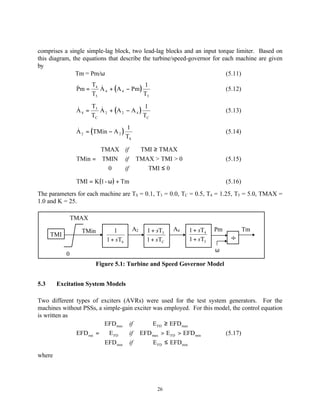
For both types of AVRs, the terminal voltage (VC), as depicted in Figure 5.3, is a function of the
d- and q-axis voltages, which, in turn, depend on the real and imaginary portions of the voltage at
the terminals (VR, VI), the current through the machine connection node (IR, II) and the
27

8. impedance seen from the machine (RC + jXC). The complete equation set for the terminal voltage
control block is given by
VC = ( VCB − VC )
& 1
(5.26)
TR
(VR + I R X C + I I R C ) + (VI + I R X C + I I R C )
2 2
VCB = (5.27)
I R   sinθ cosθ  i d 
I  = − cosθ sinθ  × i  (5.28)
 I    q
where id and iq are the d-axis and q-axis currents, respectively.
IR
II VC
1
VCB
VR 1 + sTR
VI
Figure 5.3: Terminal Voltage Control Block
5.4 Power System Stabilizer
The lead-lag PSS structure shown in Figure 5.4 was used. The control equations for this PSS are
given by
VPSSmax if &
V5 ≥ VPSSmax
&  & &
VPSS =  V5 if VPSSmax > V5 > VPSSmin (5.29)
 VPSS if & ≤ VPSS
V5
 min min
& & V
V5 = K S V3 − 5 (5.30)
TW
& T & V − V3
V3 = 3 V1 + 1 (5.31)
T4 T4
T ∆Input − V1
V1 = 1 ∆&
& Input + (5.32)
T2 T2
28

9. ∆ω = ω mach − ω o

∆Input = or (5.33)
∆Pa = P
 mech − Pelec
The parameters for the PSSs used in this thesis are given in Table 6.9, located in Section 6.3.2.
VPSSmax
∆Input 1 + sT1 V1 1 + sT3 V3 sK S TW V5 VPSS
1 + sT2 1 + sT4 1 + sTW
VPSSmin
Figure 5.4: Lead-Lag Power System Stabilizer [23]
5.5 Linearized State Equations
Now that all of the nonlinear state equations describing the system have been written, the
linearization of the state equations must be performed to yield the final form of the state space
system that is used in the small-signal stability analysis and the dynamic simulations. Concurrent
with the linearization, elimination of the non-state variables and equations from the generator
model is performed. The nonlinear equations for the generators, namely (5.3-5.6) and (5.9-5.10),
are kept as the state space model, with the elimination of the d- and q-axis current variables
completed by using (5.1), (5.2), (5.7) and (5.8). Passage from the (d, q) generator reference
frame to the (R, I) network reference frame is accomplished through the transformed current
(5.28) and the transformed voltage. The latter is written as
VR   sinΘ cosΘ  v d 
 V  = -cosΘ sinΘ  v  (5.34)
 I   q 
where VR and VI are the real and imaginary components of the network reference frame and Θ is
the angle between the network and rotor reference frames.
The complete set of state equations in matrix-vector form for the system including a machine is
now given by
29

10. &
 ∆λ f   0 a12 a13 a14 a15 a16   ∆λ f   0 b12 
 &  0 a 26   ∆λ D   0
 ∆λ D   a 22 a 23 a 24 a 25 0
   
 ∆λ Q1   0
& a32 a 33 a 34 a 35 a36   ∆λ Q1   0 0  ∆Tm 
 & = +
a 46   ∆λ Q2   0 0  ∆EFD 
(5.35)
 ∆λ Q2   0 a 42 a 43 a 44 a 45     
 ∆ω   0
& a 52 a 53 a 54 a 55 a 56   ∆ω  b41 0
      
 & 
 ∆Θ  a 61 0 0 0 0 0   ∆Θ   0 0
The equations for the simple-gain exciter from (5.18), the speed-governor control blocks from
(5.11-5.16) and the terminal voltage control block from (5.26-5.28) are not shown in this model.
The A- and B-matrix matrix coefficient expansions for the system shown in (5.35) can be found in
Appendix A, while the complete A-matrix coefficients are shown for the base case load flow in
Appendix B.
10 20 3 101 13 120 110
~ ~
GEN1 GEN11
102
~ 967 MW 1767 MW ~
GEN2 GEN12
Figure 5.5: Two Area, 4-Machine Test System
5.6 Test System
The one-line diagram of the two-area, 4-machine test system used to examine the inter-area
oscillation control problem is shown in Figure 5.5. Originally a 6-bus system in [1], the system
has been modified by the addition of transformers between each generator and the transmission
lines, and now closely resembles the 4-machine system from [11]. In fact, this system was created
especially for the analysis and study of the inter-area oscillation problem [1,11]. This system has
become a reference test system for studying the inter-area oscillation control problem, much like
the 3-machine system from [33] or the “New England” 10-machine system [35] have served as
references for other studies requiring a common, accessible test system.
Visible in the one-line diagram are the four generators, GEN1, GEN2, GEN11 and GEN12, and
their associated 20kV/230kV step-up transformers. There are two loads in the system at buses 3
30

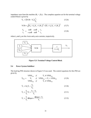
11. and 13. The transformer and line impedances for the system are given in Table 5.2, while the
generation, load and voltage data is enumerated in Table 5.3. The per-unit values were calculated
on a 100MVA base.
From Bus To Bus R (pu) X (pu) B/2 (pu)
GEN1 10 0.0 0.0167 --
GEN2 20 0.0 0.0167 --
GEN11 110 0.0 0.0167 --
GEN12 120 0.0 0.0167 --
10 20 0.0025 0.025 0.021875
20 3 0.001 0.01 0.00875
3 101 0.011 0.11 0.09625
3 102 0.011 0.11 0.09625
101 13 0.011 0.11 0.09625
102 13 0.011 0.11 0.09625
13 120 0.001 0.01 0.00875
120 110 0.0025 0.025 0.021875
Table 5.2: Impedance Data for 4-Machine System
Generator Voltage Voltage Real Reactive
or Magnitude Angle Power Power
Load (per unit) (degrees) (MW) (MVAR)
GEN1 1.03 18.56 700 185
GEN2 1.01 8.8 700 235
GEN11 1.03 -8.5 719 176
GEN12 1.01 -18.69 700 202
Load 3 0.96 -6.4 967 100
Load 13 0.97 -33.86 1767 100
Table 5.3: Initial Generation and Load Data for 4-Machine System
Many assumptions are needed to place the power system models into service for the small-signal
analysis. The loads were modeled as constant impedances. The generators were described using
the two-axis model discussed in [11] and [30] given in Section 5.1, and the turbine and speed
governor model from Section 5.2. The excitation system for each of the generators was also
modeled in detail, along with any additional controllers, as shown in Sections 5.3 and 5.4. Finally,
to complete the state matrix formulation, all of the state variables and equations were linearized
around an initial operating point, as developed in Section 5.5.
The external parameters of the generators are given in Table 5.4, while Table 5.5 contains the
exciter parameters. The initial conditions are calculated internally by EUROSTAG. However, it
is also possible to calculate these values given the generator external parameters and the load flow
results using MATLAB [36] with the program “initcond.m” (Appendix C.1), containing the
equations for the method used by EUROSTAG to calculate the initial conditions. The internal
machine parameters, consisting of the resistances and inductances, are first calculated from the set
31

12. of external parameters, including the reactances and time constants. The load flow information,
consisting of the real and reactive power generated, the machine connection bus voltage and the
angle of the voltage, is then used to calculate the initial conditions of the state variables. Based on
this approach, Table 5.6 contains the internal parameters of the generators and Table 5.7 the
initial conditions.
Parameter Generators 1, 2 Generators 11, 12
xd 1.8 1.8
x’d 0.3 0.3
x’’d 0.25 0.25
xq 1.7 1.7
x’q 0.55 0.55
x’’q 0.25 0.25
Ra 0.0025 0.0025
Xl 0.2 0.2
T’do 8.0 8.0
T’’do 0.03 0.03
T’qo 0.4 0.4
T’’qo 0.05 0.05
H 6.5 6.175
Table 5.4: External Parameter Generator Data
Parameter Value
KA 345.1265
TA 0.0116
KF 0.0551
TF 2.1511
VImax 12.137
VImin -12.137
EFDmax Vterm(12.137) - Ifield
EFDmin Vterm(-12.137) + Ifield
RC 0.0
XC 0.0
TR 0.01
Table 5.5: ST1-Type Exciter Data
32

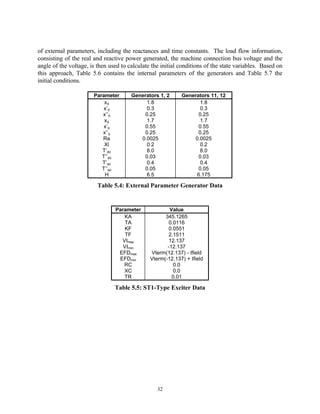
13. Parameter Gen 1,2, 11,12,
Ra 0.0025
Ld 0.2
Lq 0.2
rf 0.0006
rD 0.0172
rQ1 0.0231
rQ2 0.0241
Lf 0.1123
LD 0.0955
LQ1 0.0547
LQ2 0.9637
Md 1.6
Mq 1.5
Table 5.6: Internal Machine Parameters
Parameter Gen 1 Gen 2 Gen 12 Gen 11
URo -0.2941 0.5908 0.1065 -0.8224
UIo 0.9871 -0.8192 0.9972 -0.6201
IRo -0.0267 0.2648 0.3749 -0.8052
IIo 0.8569 -0.8511 0.7957 -0.3461
udo -0.9953 0.9572 -0.97 1.0
uqo 0.6927 -0.2182 1.0464 -0.5672
ido -0.1045 0.1087 0.1073 0.1069
iqo 0.1044 -0.0896 0.0682 0.0737
Θo 0.0293 0.3 -0.442 -1.1667
λado 0.0191 -0.0212 0.0187 -0.0199
λaqo 0.0235 -0.0205 0.0162 0.0121
λQ1o 0.0235 -0.0205 0.0162 0.0121
λQ2o 0.0235 -0.0205 0.0162 0.0121
λdo 0.1355 -0.1431 0.1376 -0.1392
λqo 0.0322 -0.0349 0.032 -0.0333
ifo 0.1165 -0.1219 0.1189 -0.1193
efdo -0.1863 0.1951 -0.1903 0.1909
tmo -0.0005 -0.0005 -0.0004 0.0003
Table 5.7: Generator Initial Conditions
EUROSTAG was also used to perform the small-signal and time-domain analyses. In brief, this
package calculates the load flow based on the topological data of the power system, then uses the
parameters of the machines in the system coupled with the load flow results to perform the time-
domain simulations. While small-signal analysis is not included in the operational functions of this
package, it is possible to save the state-space model at any instant in time during the dynamic
simulations in a format compatible with that of MATLAB [32]. The use of MATLAB in
conjunction with EUROSTAG provides the tools needed to complete the analysis of the research
performed in this thesis.
33

14. There are, however, several drawbacks to using the two software packages in this manner. It is
not possible to explicitly see the state equations as they are used in the eigenvalue calculation and
the time-domain simulation. However, it is possible to write all of the equations describing the
machines and their interactions used by the software. While the Y-bus matrix is also not available
as a EUROSTAG output, the derivation of this matrix can be performed in the manner described
in [33]. The discussion of a multi-machine stability problem is given in [33] as well, and this
reference is quoted by the EUROSTAG programmers [30, 32].
34