ch06.pptx

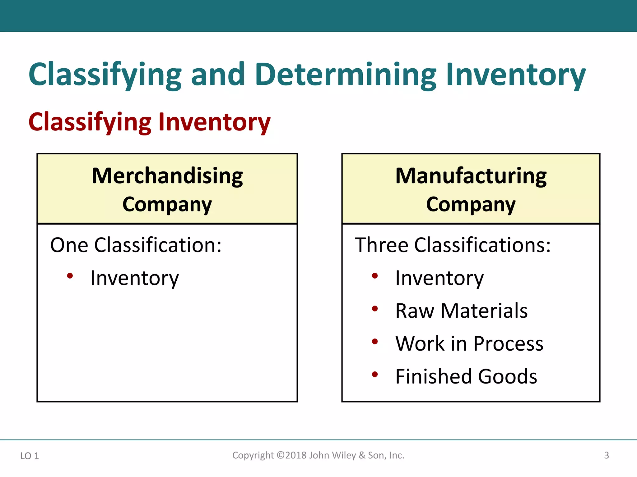
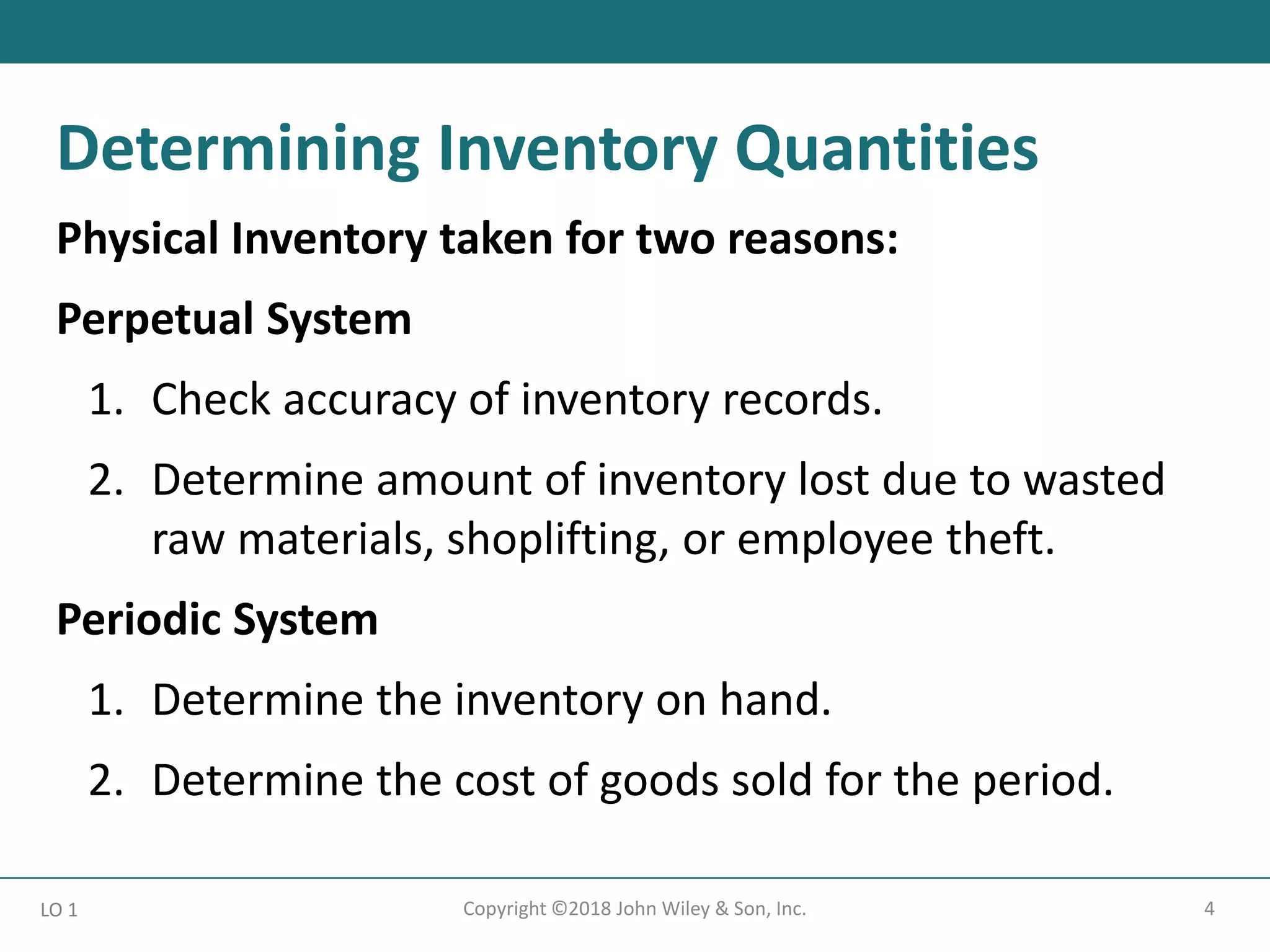
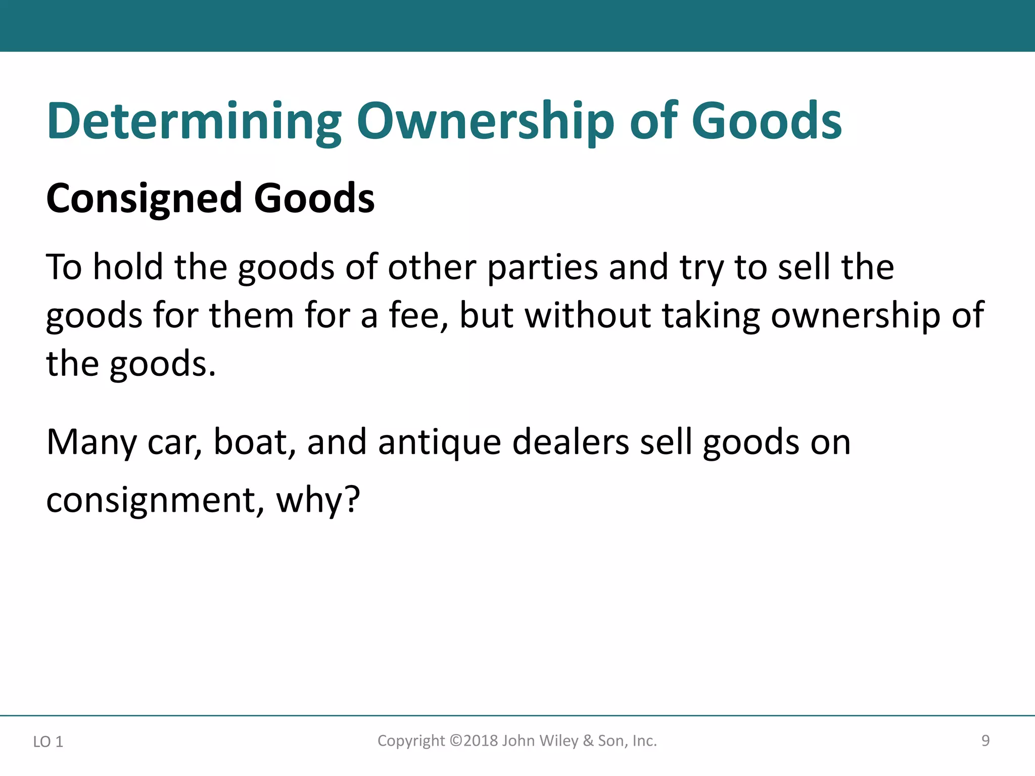
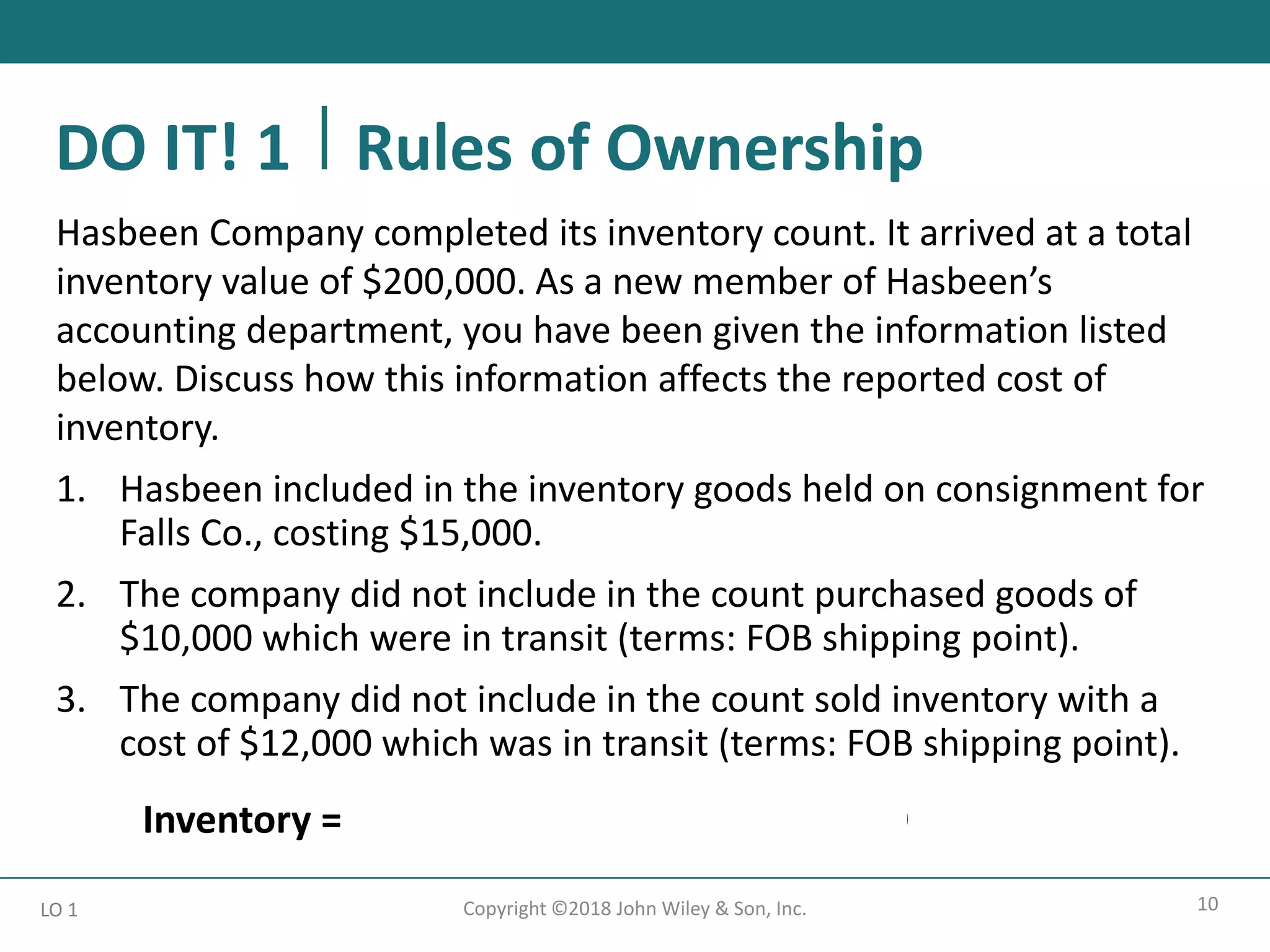
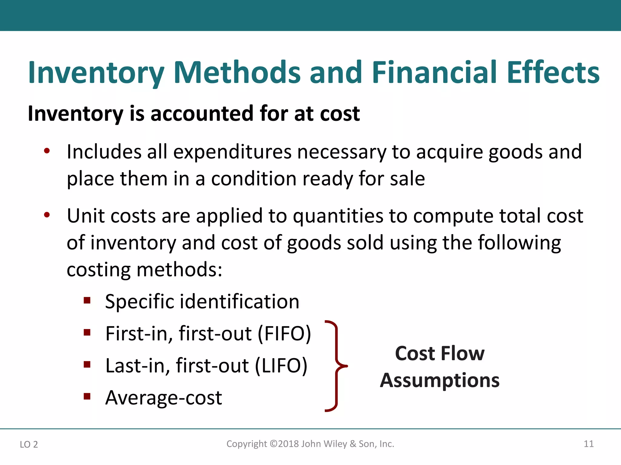
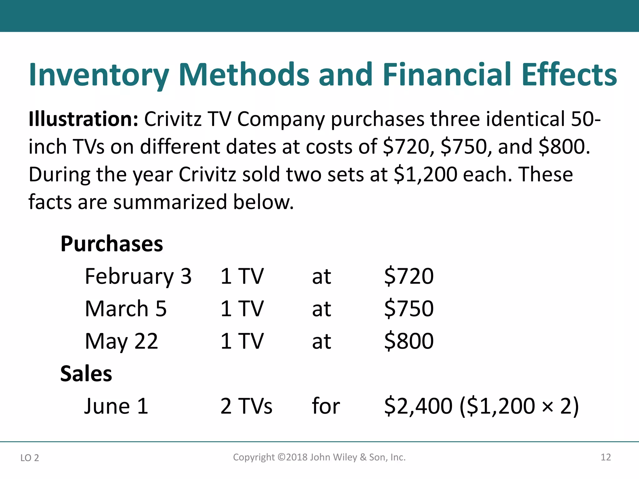
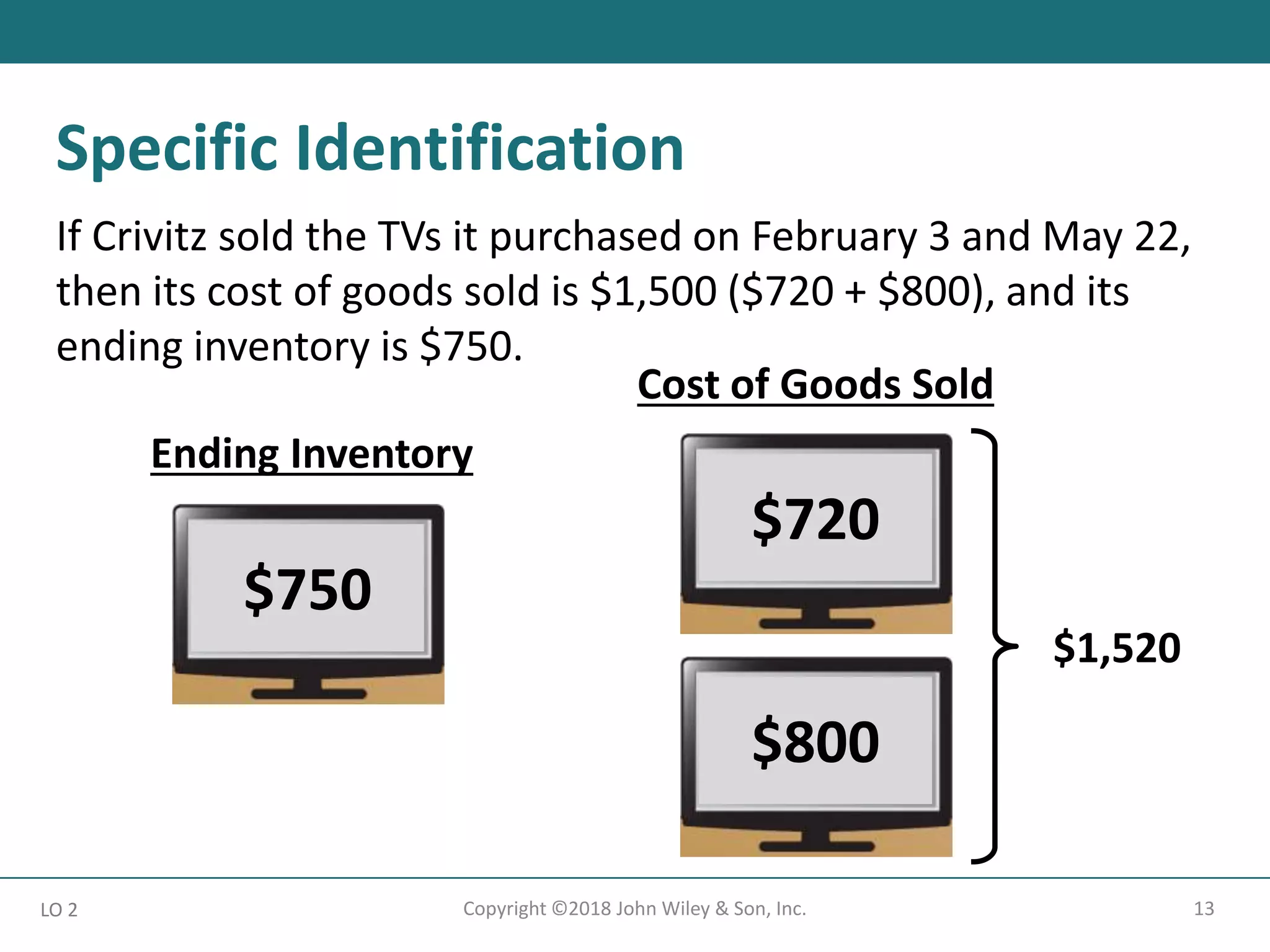
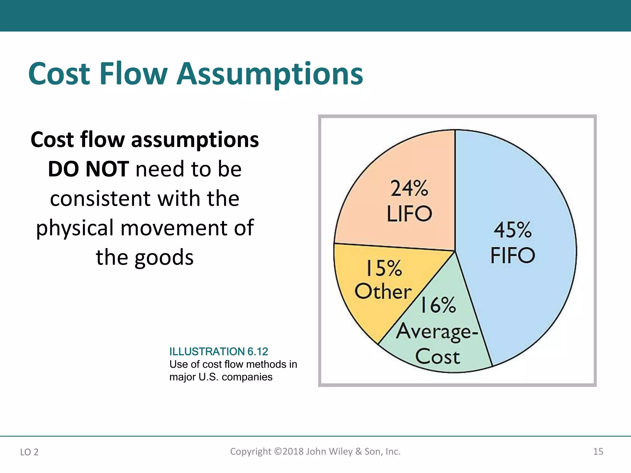
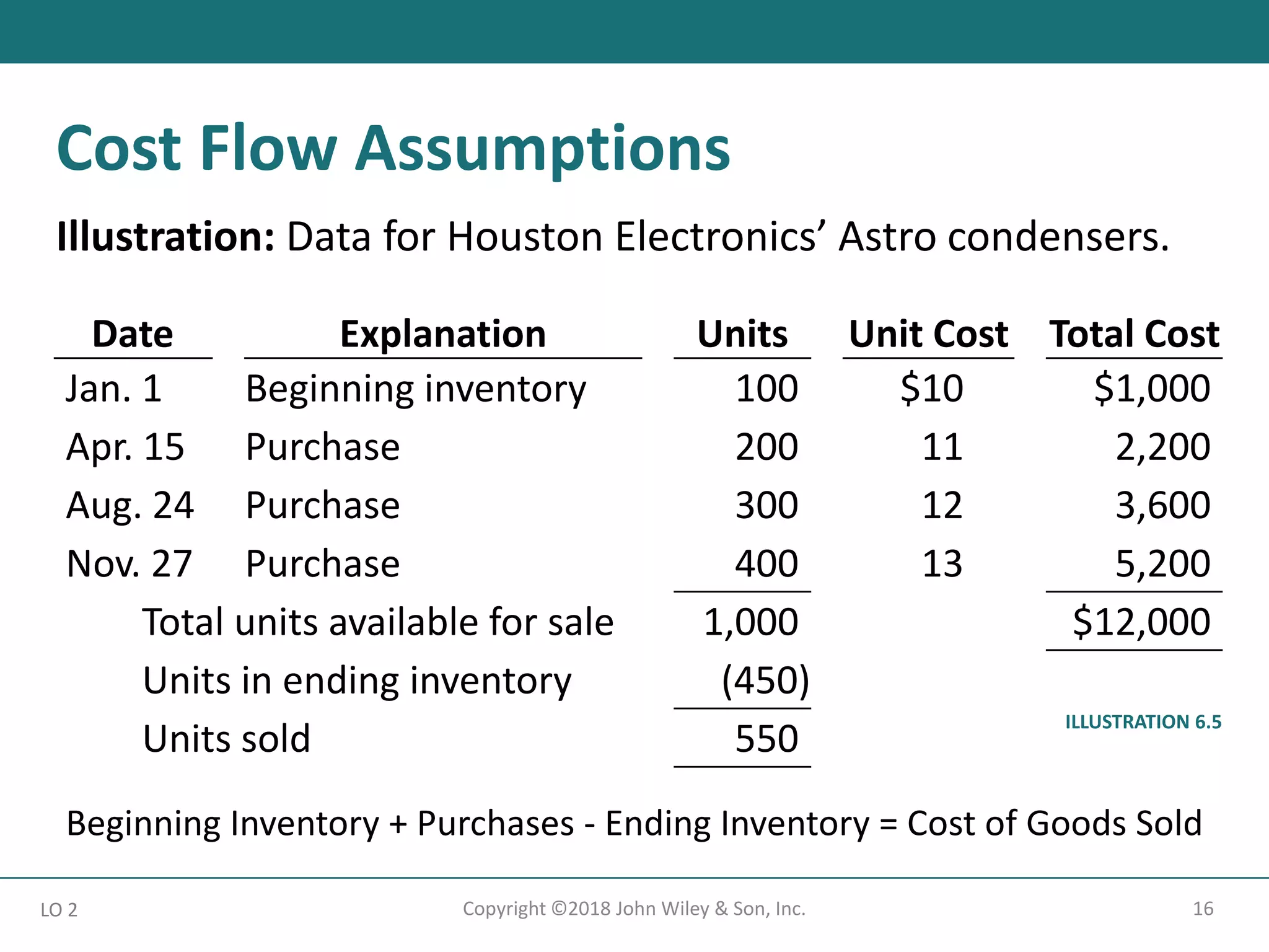
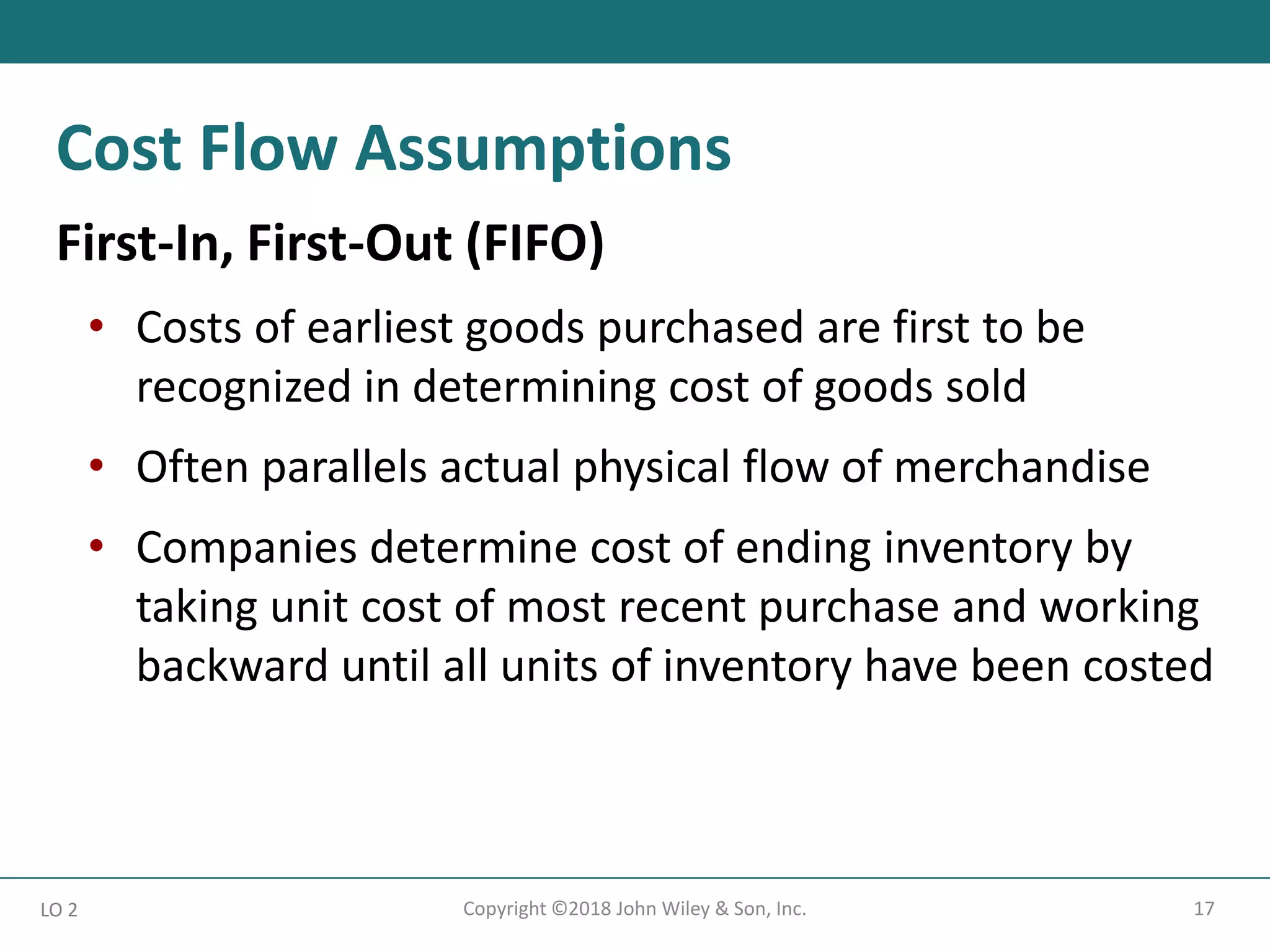
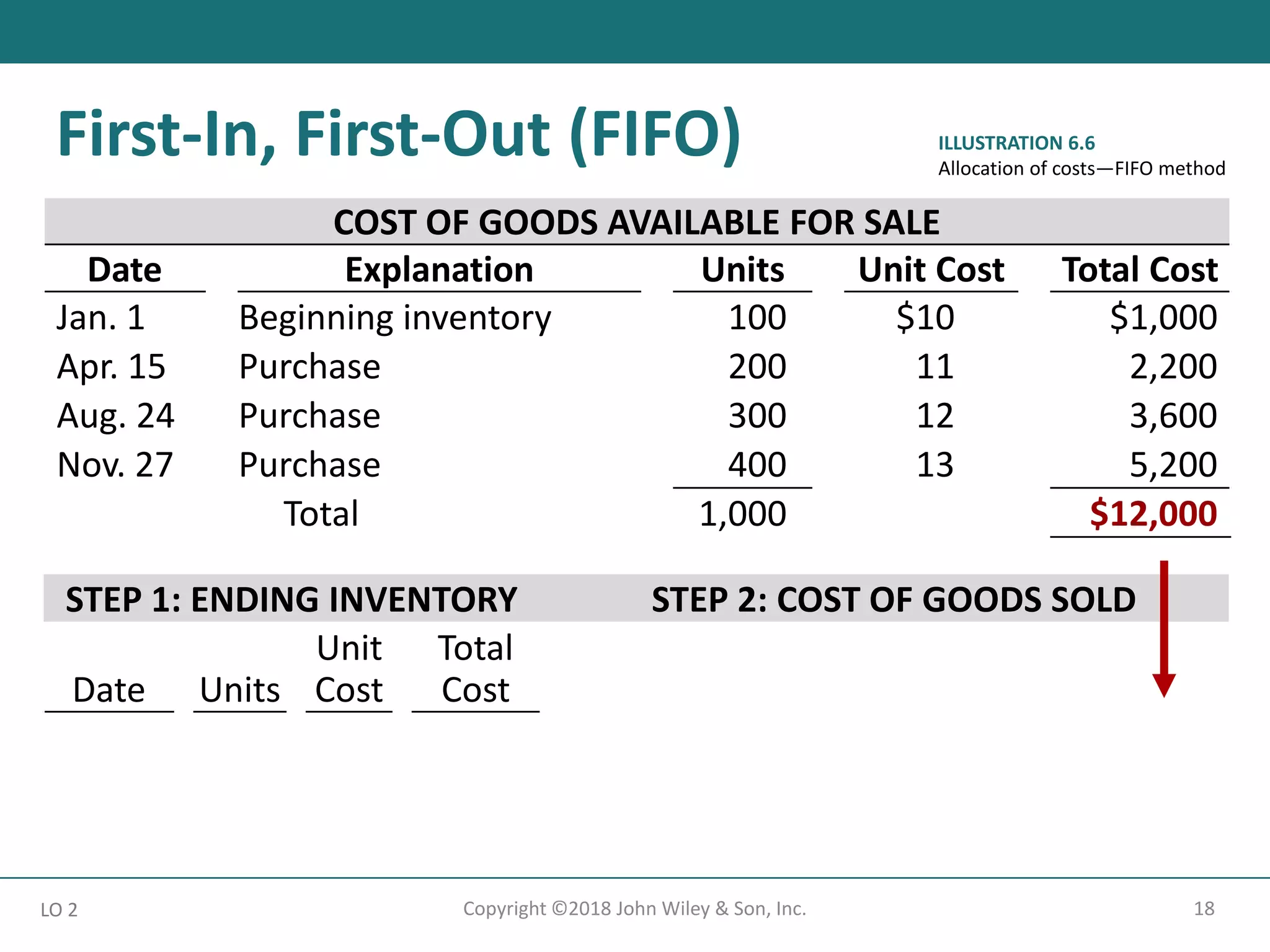
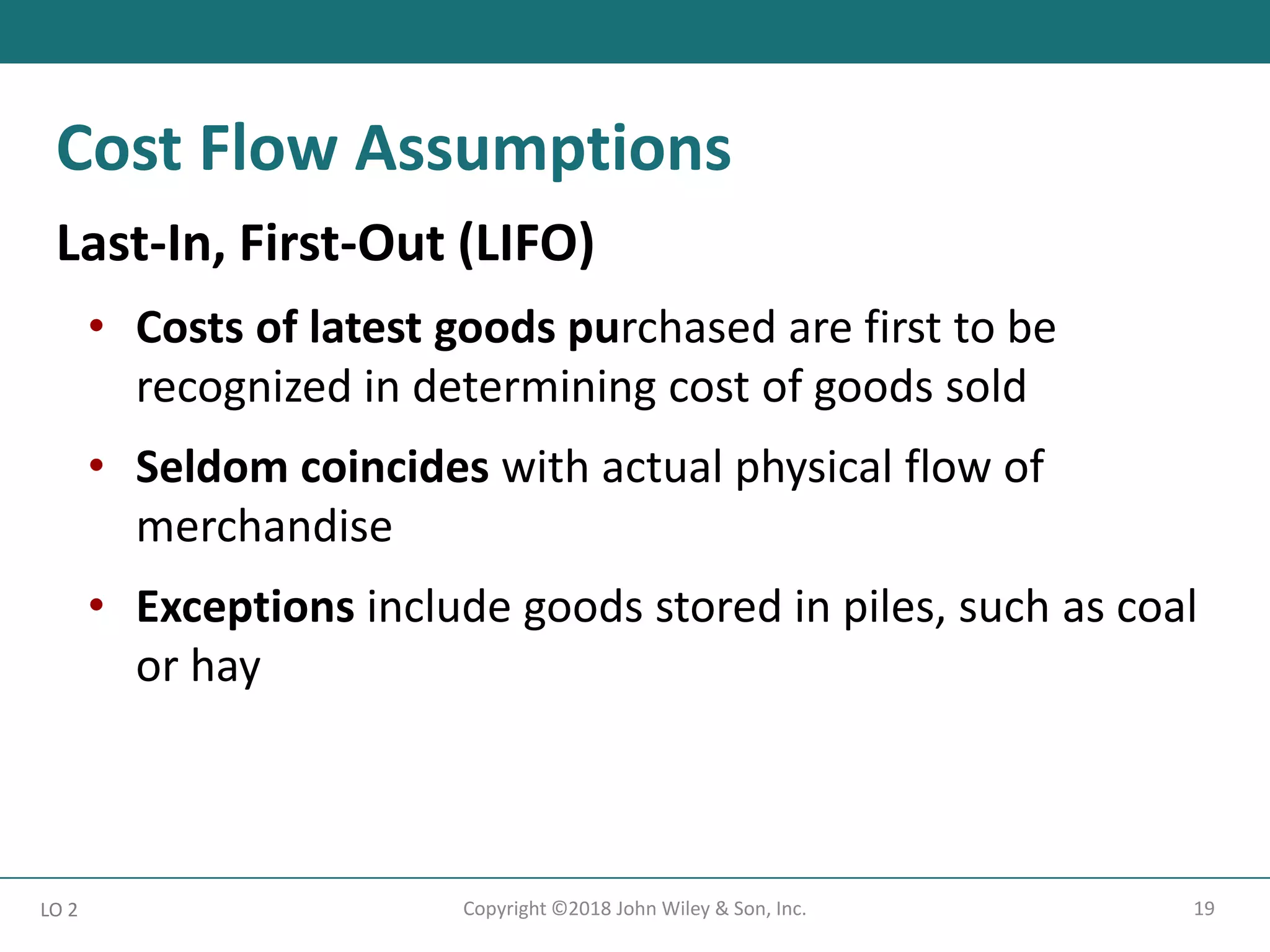
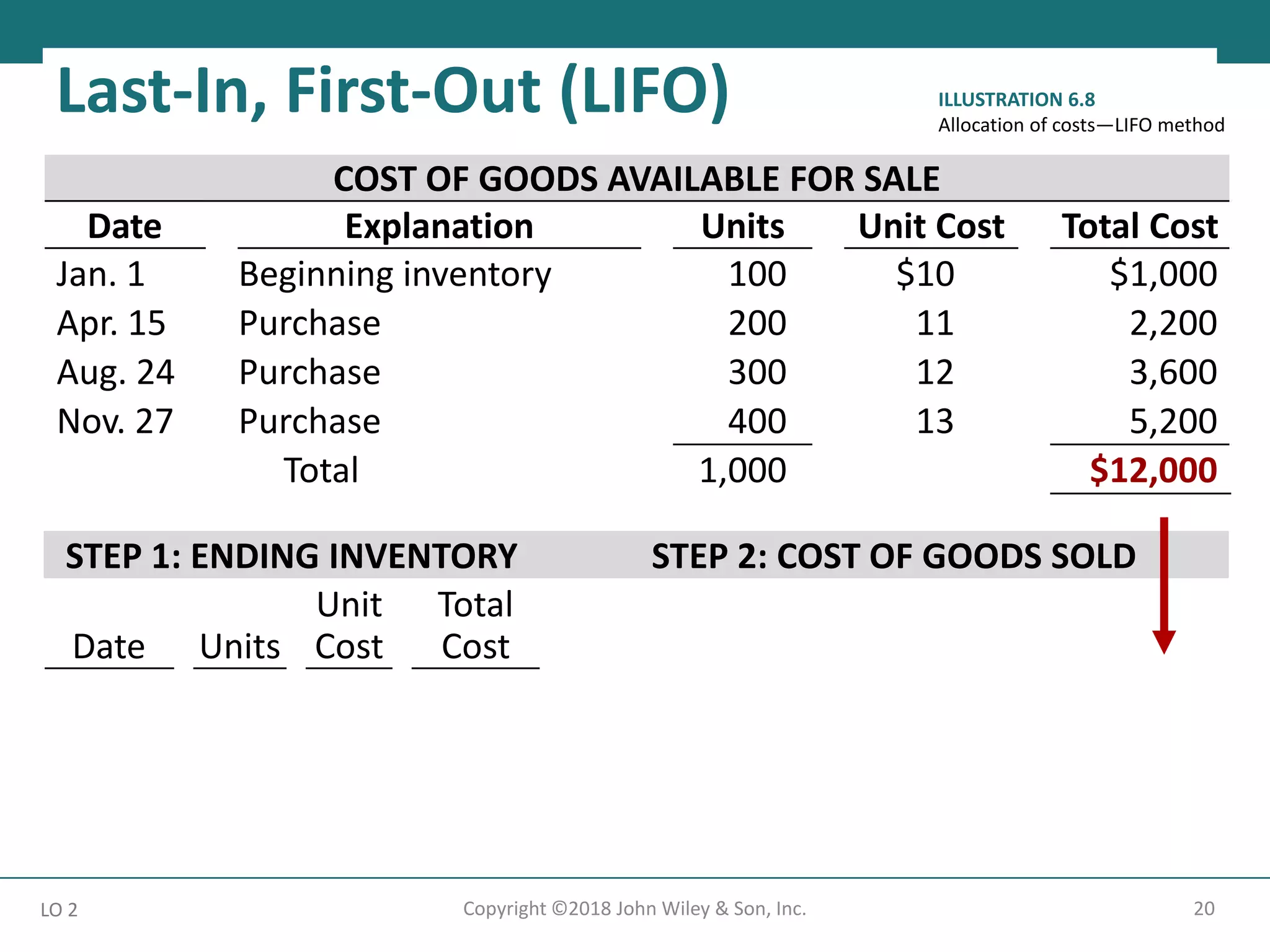
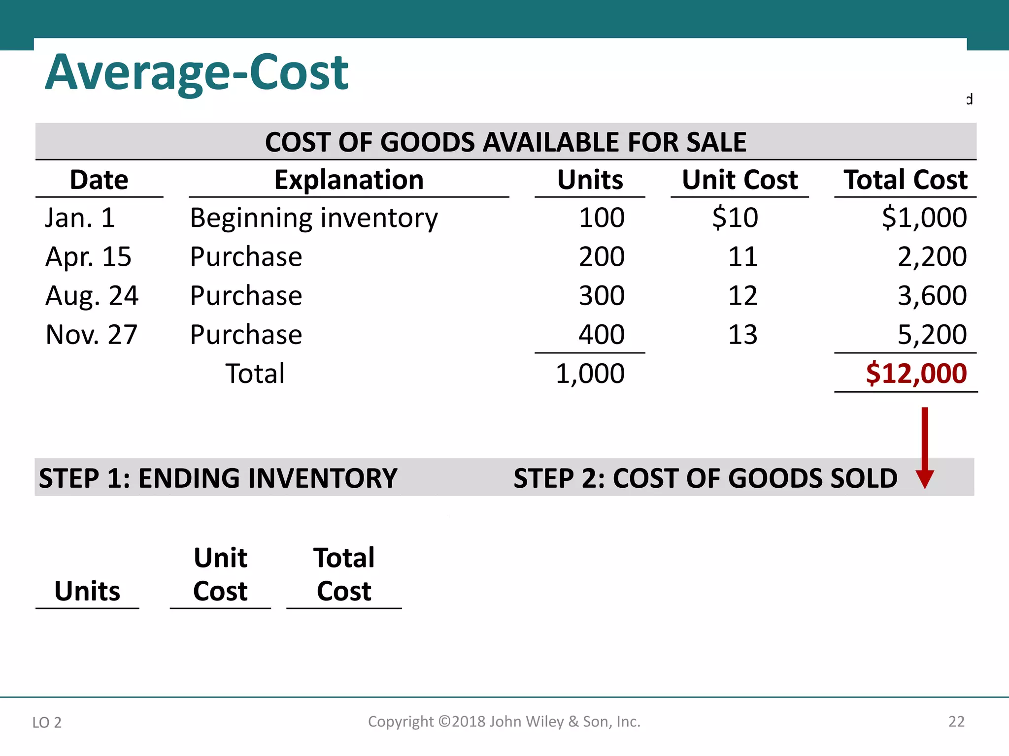
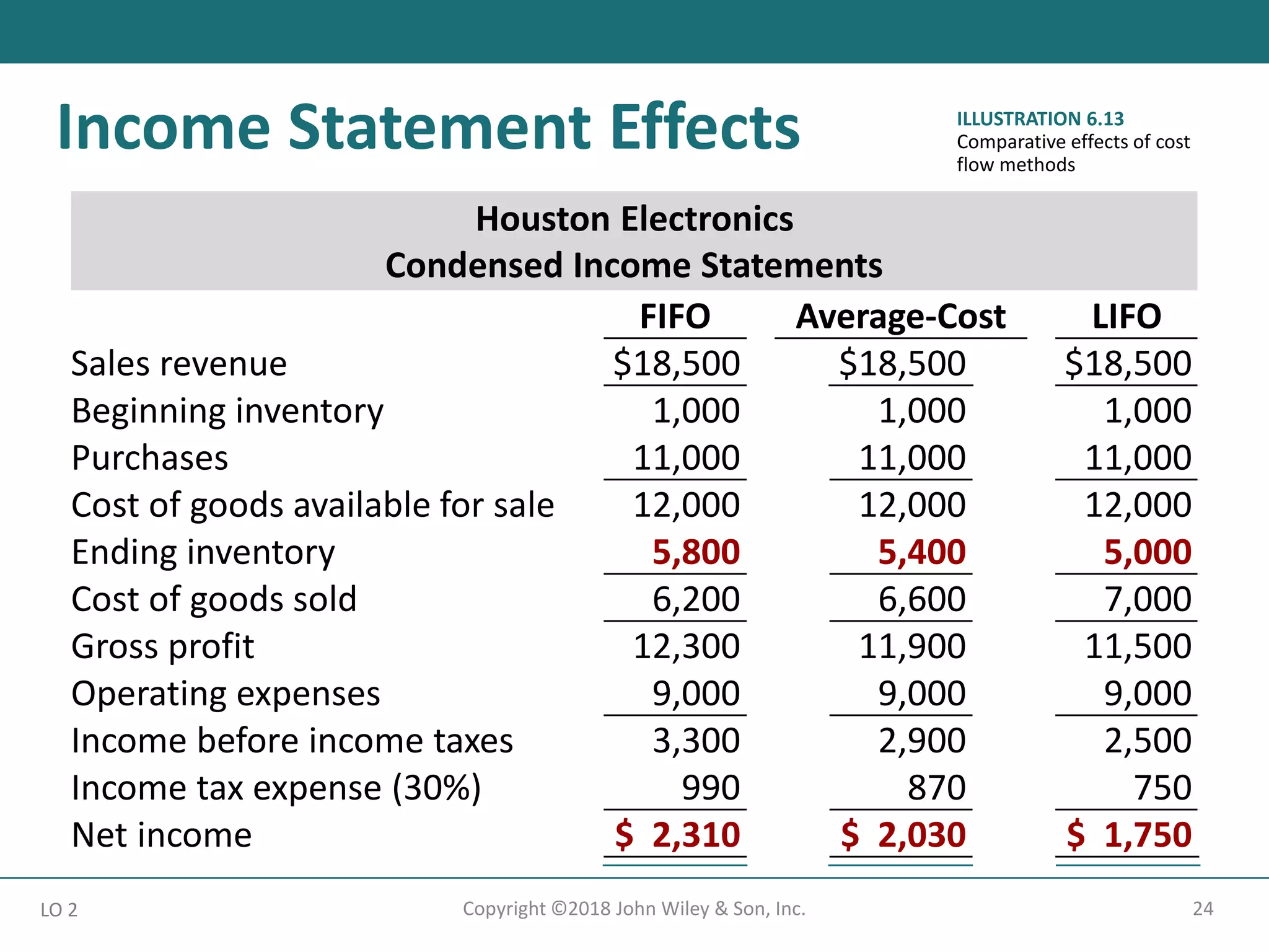
Accounting Principles
Thirteenth Edition
Weygandt Kimmel Kieso
Chapter 6
Inventories
Prepared by
Coby Harmon
University of California, Santa Barbara
Westmont College

Chapter Outline
Learning Objectives
LO 1 Discuss how to classify and determine inventory.
LO 2 Apply inventory cost flow methods and discuss
their financial effects.
LO 3 Indicate the effects of inventory errors on the
financial statements.
LO 4 Explain the statement presentation and analysis of
inventory.
2
Copyright ©2018 John Wiley & Son, Inc.

Classifying and Determining Inventory
3
LO 1
Classifying Inventory
Merchandising
Company
Manufacturing
Company
One Classification:
• Inventory
Three Classifications:
• Inventory
• Raw Materials
• Work in Process
• Finished Goods

4
Physical Inventory taken for two reasons:
Perpetual System
1. Check accuracy of inventory records.
2. Determine amount of inventory lost due to wasted
raw materials, shoplifting, or employee theft.
Periodic System
1. Determine the inventory on hand.
2. Determine the cost of goods sold for the period.
LO 1
Determining Inventory Quantities

5
Taking a Physical Inventory
Involves counting, weighing, or measuring each kind of
inventory on hand.
Companies often “take inventory”
• when business is closed or business is slow
• at the end of accounting period
LO 1

6
Determining Ownership of Goods
Goods in Transit
• Purchased goods not yet received
• Sold goods not yet delivered
• Included in inventory of company that has legal title
to goods
LO 1

7
LO 1
Goods in Transit
ILLUSTRATION 6.2
Terms of sale
Ownership of goods
passes to buyer when
public carrier accepts
goods from seller.
Ownership of goods
remains with seller until
the goods reach buyer.
Freight costs incurred by the seller are an operating expense.

8
Goods in transit should be included in the inventory of
the buyer when the:
a. public carrier accepts the goods from the seller
b. goods reach the buyer
c. terms of sale are FOB destination
d. terms f sale are FOB shipping point
LO 1
Goods in Transit

9
Consigned Goods
To hold the goods of other parties and try to sell the
goods for them for a fee, but without taking ownership of
the goods.
Many car, boat, and antique dealers sell goods on
consignment, why?
LO 1
Determining Ownership of Goods

10
Hasbeen Company completed its inventory count. It arrived at a total
inventory value of $200,000. As a new member of Hasbeen’s
accounting department, you have been given the information listed
below. Discuss how this information affects the reported cost of
inventory.
1. Hasbeen included in the inventory goods held on consignment for
Falls Co., costing $15,000.
2. The company did not include in the count purchased goods of
$10,000 which were in transit (terms: FOB shipping point).
3. The company did not include in the count sold inventory with a
cost of $12,000 which was in transit (terms: FOB shipping point).
Inventory = $200,000 - $15,000 + $10,000 = $195,000
LO 1
DO IT! 1 Rules of Ownership

11
Inventory is accounted for at cost
• Includes all expenditures necessary to acquire goods and
place them in a condition ready for sale
• Unit costs are applied to quantities to compute total cost
of inventory and cost of goods sold using the following
costing methods:
 Specific identification
 First-in, first-out (FIFO)
 Last-in, first-out (LIFO)
 Average-cost
LO 2
Inventory Methods and Financial Effects
Cost Flow
Assumptions

12
Illustration: Crivitz TV Company purchases three identical 50-
inch TVs on different dates at costs of $720, $750, and $800.
During the year Crivitz sold two sets at $1,200 each. These
facts are summarized below.
Purchases
February 3 1 TV at $720
March 5 1 TV at $750
May 22 1 TV at $800
Sales
June 1 2 TVs for $2,400 ($1,200 × 2)
LO 2
Inventory Methods and Financial Effects

13
If Crivitz sold the TVs it purchased on February 3 and May 22,
then its cost of goods sold is $1,500 ($720 + $800), and its
ending inventory is $750.
LO 2
Specific Identification
$750
$720
$800
Cost of Goods Sold
Ending Inventory
$1,520

14
Costing method in which items still in inventory are
specifically costed to arrive at the total cost of the ending
inventory.
• Practice is relatively rare
• Most companies make assumptions (cost flow
assumptions) about which units were sold
LO 2
Specific Identification

15
Cost flow assumptions
DO NOT need to be
consistent with the
physical movement of
the goods
LO 2
Cost Flow Assumptions
ILLUSTRATION 6.12
Use of cost flow methods in
major U.S. companies

Date Explanation Units Unit Cost Total Cost
Jan. 1 Beginning inventory 100 $10 $1,000
Apr. 15 Purchase 200 11 2,200
Aug. 24 Purchase 300 12 3,600
Nov. 27 Purchase 400 13 5,200
Total units available for sale 1,000 $12,000
Units in ending inventory (450)
Units sold 550
Beginning Inventory + Purchases - Ending Inventory = Cost of Goods Sold
16
Illustration: Data for Houston Electronics’ Astro condensers.
LO 2
ILLUSTRATION 6.5

17
First-In, First-Out (FIFO)
• Costs of earliest goods purchased are first to be
recognized in determining cost of goods sold
• Often parallels actual physical flow of merchandise
• Companies determine cost of ending inventory by
taking unit cost of most recent purchase and working
backward until all units of inventory have been costed
LO 2

18
LO 2
ILLUSTRATION 6.6
Allocation of costs—FIFO method
COST OF GOODS AVAILABLE FOR SALE
Apr. 15 Purchase 200 11 2,200
Aug. 24 Purchase 300 12 3,600
Nov. 27 Purchase 400 13 5,200
Total 1,000 $12,000
STEP 1: ENDING INVENTORY STEP 2: COST OF GOODS SOLD
Date Units
Unit
Cost
Total
Cost
Nov. 27 400 $13 $5,200 Cost of goods available for sale $12,000
Aug. 24 50 12 600 Less : Ending inventory 5,800
Total 450 $5,800 Cost of goods sold $ 6,200

19
Last-In, First-Out (LIFO)
• Costs of latest goods purchased are first to be
recognized in determining cost of goods sold
• Seldom coincides with actual physical flow of
merchandise
• Exceptions include goods stored in piles, such as coal
or hay
LO 2

Date Units
Unit
Cost
Total
Cost
Jan. 1 100 $10 $1,000 Cost of goods available for sale $12,000
Apr. 15 200 11 2,200 Less : Ending inventory 5,000
Aug. 24 150 12 1,800 Cost of goods sold $ 7,000
Total 450 $5,000
Last-In, First-Out (LIFO)
20
LO 2
ILLUSTRATION 6.8
Allocation of costs—LIFO method
Apr. 15 Purchase 200 11 2,200
Aug. 24 Purchase 300 12 3,600
Nov. 27 Purchase 400 13 5,200
Total 1,000 $12,000

21
Average-Cost
• Allocates cost of goods available for sale on basis of
weighted-average unit cost incurred
• Applies weighted-average unit cost to units on hand
to determine cost of ending inventory
LO 2

$12,000 ÷ 1,000 = $12 Cost of goods available for sale $12,000
Units
Unit
Cost
Total
Cost
Less : Ending inventory
Cost of goods sold
5,400
$ 6,600
450 $12 $5,400
22
LO 2
ILLUSTRATION 6.8
Allocation of costs—LIFO method
Apr. 15 Purchase 200 11 2,200
Aug. 24 Purchase 300 12 3,600
Nov. 27 Purchase 400 13 5,200
Total 1,000 $12,000
Average-Cost

23
Each of the three cost flow methods is acceptable for use.
• Reebok International Ltd. and Wendy’s International
currently use the FIFO method
• Campbell Soup Company, Krogers, and Walgreen Drugs
use LIFO for part or all of their inventory
• Bristol-Myers Squibb, Starbucks, and Motorola use the
average-cost method
• Stanley Black & Decker Manufacturing Company uses
LIFO for domestic inventories and FIFO for foreign
inventories
LO 2
Financial Statement and Tax Effects
of Cost Flow Methods

24
LO 2
Income Statement Effects
Houston Electronics
Condensed Income Statements
FIFO Average-Cost LIFO
Sales revenue $18,500 $18,500 $18,500
Beginning inventory 1,000 1,000 1,000
Purchases 11,000 11,000 11,000
Cost of goods available for sale 12,000 12,000 12,000
Ending inventory 5,800 5,400 5,000
Cost of goods sold 6,200 6,600 7,000
Gross profit 12,300 11,900 11,500
Operating expenses 9,000 9,000 9,000
Income before income taxes 3,300 2,900 2,500
Income tax expense (30%) 990 870 750
Net income $ 2,310 $ 2,030 $ 1,750
ILLUSTRATION 6.13
Comparative effects of cost
flow methods

25
• A major advantage of the FIFO method is that in a
period of inflation, costs allocated to ending
inventory will approximate their current cost
• A major shortcoming of the LIFO method is that in a
period of inflation, costs allocated to ending
inventory may be significantly understated in terms of
current cost
LO 2
Balance Sheet Effects

26
• Both inventory and net income are higher when
companies use FIFO in a period of inflation
• LIFO results in the lowest income taxes (because of
lower net income) during times of rising prices
• A tax rule requires that if companies use LIFO for tax
purposes they must also use it for financial reporting
purposes (LIFO conformity rule)
LO 2
Tax Effects

27
• Method should be used consistently, enhances
comparability
• Although consistency is preferred, a company may
change its inventory costing method
LO 2
Using Inventory Cost Flow Methods
Consistently
Quaker Oats
Notes to the Financial Statements
Note 1: Effective July 1, the Company adopted the LIFO cost flow assumption for
valuing the majority of U.S. Grocery Products inventories. The Company believes that
the use of the LIFO method better matches current costs with current revenues. The
effect of this change on the current year was to decrease net income by $16.0 million.
ILLUSTRATION 6.14
Disclosure of change in cost flow method

28
The cost flow method that often parallels the actual
physical flow of merchandise is the:
a. FIFO method
b. LIFO method
c. average cost method
d. gross profit method
LO 2

29
In a period of inflation, the cost flow method that
results in the lowest income taxes is the:
a. FIFO method
b. LIFO method
c. average cost method
d. gross profit method
LO 2

30
LO 2
DO IT! 2 Cost Flow Methods
The accounting records of Shumway Ag Implements show the
following data.
Beginning inventory 4,000 units at $ 3
Purchases 6,000 units at $ 4
Sales 7,000 units at $12
Determine the cost of goods sold during the period under a
periodic inventory system using (a) the FIFO method, (b) the
LIFO method, and (c) the average-cost method.

Units
Unit
Cost
Total
Cost
Cost of goods available for sale $36,000
Less : Ending inventory 12,000
3,000 $4 $12,000 Cost of goods sold $ 24,000
31
LO 2
Beginning inventory 4,000 $ 3 $12,000
Purchase 6,000 4 24,000
Total 10,000 $36,000
DO IT! 2 FIFO Method
Determine cost of goods sold under a periodic inventory.

Units
Unit
Cost
Total
Cost
3,000 $3 $9,000 Cost of goods sold $ 27,000
32
LO 2
Beginning inventory 4,000 $ 3 $12,000
Purchase 6,000 4 24,000
Total 10,000 $36,000
DO IT! 2 LIFO Method

Units
Unit
Cost
Total
Cost
3,000 $3.60 $10,800 Cost of goods sold $ 25,200
33
LO 2
Beginning inventory 4,000 $3.00 $12,000
Purchase 6,000 4.00 24,000
Total 10,000 $3.60 $36,000
DO IT! 2 Average-Cost Method
Average Cost Per Unit

34
Common Cause:
• Failure to count or price inventory correctly
• Not properly recognizing the transfer of legal title to
goods in transit
• Errors affect both the income statement and balance
sheet
LO 3
Effects of Inventory Errors

35
Inventory errors affect the computation of cost of goods
sold and net income in two periods.
LO 3
Effects of Inventory Errors
Beginning
Inventory
+
Cost of
Goods
Purchased
-
Ending
Inventory
=
Cost of
Goods
Sold
When Inventory Error:
Cost of
Goods Sold Is: Net Income Is:
Understates beginning inventory Understated Overstated
Overstates beginning inventory Overstated Understated
Understates ending inventory Overstated Understated
Overstated ending inventory Understated Overstated
ILLUSTRATION 6.16
Effects of inventory errors on current year’s income statement
ILLUSTRATION 6.15
Formula for cost of goods sold

36
Inventory errors affect the computation of cost of goods
sold and net income in two periods.
• An error in ending inventory of current period will
have a reverse effect on net income of next
accounting period
• Over two years, total net income is correct because
errors offset each other
• Ending inventory depends entirely on accuracy of
taking and costing inventory
LO 3

37
LO 3
($3,000)
Understated
$3,000
Overstated
Combined income
for 2-year period is
correct.
ILLUSTRATION 6.17
Effects of inventory errors on
two years’ income statements
2019 2020
Incorrect Correct Incorrect Correct
Sales $ 80,000 $ 80,000 $ 90,000 $ 90,000
Beginning inventory 20,000 20,000 12,000 15,000
Cost of goods purchased 40,000 40,000 68,000 68,000
Cost of goods available 60,000 60,000 80,000 83,000
Ending inventory 12,000 15,000 23,000 23,000
Cost of good sold 48,000 45,000 57,000 60,000
Gross profit 32,000 35,000 33,000 30,000
Operating expenses 10,000 10,000 20,000 20,000
Net income $ 22,000 $ 25,000 $ 13,000 $ 10,000

38
Understating ending inventory will overstate:
a. assets
b. cost of goods sold
c. net income
d. stockholders’ equity
LO 3

39
Effect of inventory errors on the balance sheet is
determined by using the basic accounting equation:
Assets = Liabilities + Stockholders’ Equity.
Errors in the ending inventory have the following effects.
LO 3
Balance Sheet Effects
Ending
Inventory Error Assets Liabilities
Stockholders’
Equity
Overstated
Understated
Overstated
Understated
No effect
No effect
Overstated
Understated
ILLUSTRATION 6.18
Effects of ending inventory errors on balance sheet

2019 2020
Ending inventory $22,000 overstated No effect
Cost of goods sold $22,000 understated $22,000 overstated
Owner’s equity $22,000 overstated No effect
40
Visual Company overstated its 2019 ending inventory by
$22,000. Determine the impact this error has on ending
inventory, cost of goods sold, and owner’s equity in 2019 and
2020.
Solution
LO 3
DO IT! 3 Inventory Errors

41
Presentation
Balance Sheet - Inventory classified as current asset.
Income Statement - Cost of goods sold subtracted from
sales.
There also should be disclosure of
1. major inventory classifications
2. basis of accounting (cost or LCM)
3. costing method (FIFO, LIFO, or average-cost)
LO 4
Statement Presentation and Analysis

42
When the value of inventory is lower than its cost
• Companies must “write down” inventory to its net
realizable value
• Net realizable value: Amount that company expects
to realize (receive from the sale of inventory)
• Example of conservatism
LO 4
Lower-of-Cost-or-Net Realizable Value

43
Illustration: Assume that Ken Tuckie TV has the following lines
of merchandise with costs and market values as indicated.
LO 4
Lower-of-Cost-or-Net Realizable Value
Units
Cost
per Unit
Net
Realizable
Value per Unit
Lower-of-Cost-or-Net
Realizable Value
Flat-screen TVs 100 $600 $550 $ 55,000 ($550 x 100)
Satellite radios 500 90 104 45,000 ($90 x 500)
DVD recorders 850 50 48 40,800 ($48 x 850)
DVDs 3,000 5 6 15,000 ($5 x 3,000)
Total inventory $155,800
ILLUSTRATION 6.19
Computation of lower-of-cost-or-net realizable value

44
Analysis
Inventory management is a double-edged sword
1. High Inventory Levels - may incur high carrying
costs (e.g., investment, storage, insurance,
obsolescence, and damage).
2. Low Inventory Levels – may lead to stock-outs and
lost sales.
LO 4
Statement Presentation and Analysis

45
LO 4
Analysis
Inventory turnover measures the number of times on
average the inventory is sold during the period.
Cost of Goods Sold
Average Inventory
Inventory
Turnover
=
Days in inventory measures the average number of
days inventory is held.
Days in Year (365)
Inventory Turnover
Days in
Inventory
=

46
LO 4
Analysis
Illustration: Wal-Mart reported in its 2016 annual report a
beginning inventory of $45,141 million, an ending inventory of
$44,469 million, and cost of goods sold for the year ended
January 31, 2016, of $360,984 million. The inventory turnover
formula and computation for Wal-Mart are shown below.
Cost of
Goods Sold
÷ Average Inventory = Inventory Turnover
$360,984 ÷
$44,469 + $45,141
= 8.1 Times
2
ILLUSTRATION 6.20
Inventory turnover formula and computation for Wal-Mart 365 ÷ 8.1 = 45.1 Days

47
LO 4
DO IT! 4 LCNRV
Tracy company sells three different types of home heating stoves
(gas, wood, and pellet). The cost and net realizable value of its
inventory of stoves are as follows.
Cost Net Realizable Value
Gas $ 84,000 $ 79,000
Wood 250,000 280,000
Pellet 112,000 101,000
Determine the value of the company’s inventory under the lower-
of-cost-or-net realizable value approach.
Solution: The lowest value for each inventory type is gas $79,000,
wood $250,000, and pellet $101,000. The total inventory value is
the sum of these amounts, $430,000.

48
LO 4
DO IT! 4 Inventory Turnover
Early in 2020, Westmoreland Company switched to a just-in-time
inventory system. Its sales revenue, cost of goods sold, and
inventory amounts for 2019 and 2020 are shown below.
2019 2020
Sales revenue $2,000,000 $1,800,000
Cost of goods sold 1,000,000 910,000
Beginning inventory 290,000 210,000
Ending inventory 210,000 50,000
Determine the inventory turnover and days in inventory for 2019
and 2020.

2019 2020
Sales revenue $2,000,000 $1,800,000
Cost of goods sold 1,000,000 910,000
Beginning inventory 290,000 210,000
Ending inventory 210,000 50,000
49
LO 4
Inventory
turnover
2019 2020
$1,000,000
= 4
$44,469 + $45,141 =7
($290,000 + $210,000)/2 2
Days in
inventory
365 ÷ 4 = 91.3 Days 365 ÷ 7 = 52.1 Days
DO IT! 4 Inventory Turnover

50
LO 5
Appendix 6A Inventory Methods and the
Perpetual System
Illustration: Compute Cost of Goods Sold and Ending Inventory under
FIFO, LIFO, and average-cost.
ILLUSTRATION 6A.1
Inventoriable units and costs
HOUSTON ELECTRONICS
Balance
in Units
1/1 Beginning inventory 100 $10 $ 1,000 100
4/15 Purchase 200 11 2,200 300
8/24 Purchase 300 12 3,600 600
9/10 Sale 550 50
11/27 Purchase 400 13 5,200 450
$12,000

Date Purchases
Cost of
Goods Sold Inventory Balance
1/1 (100 @ $10) $1,000
4/15 (200 @ $11) $2,200 (100 @ $10)
$3,200
(200 @ $11)
8/ 24 (300 @ $12) $3,600 (100 @ $10)
(200 @ $11) $6,800
(300 @ $12)
9/10 (100 @ $10)
(200 @ $11)
(250 @ $12) ( 50 @ $12) $600
$6,200
11/27 (400 @ $13) $5,200 ( 50 @ $12)
$5,800
(400 @ $13)
51
LO 5
ILLUSTRATION 6A.2
Perpetual system—FIFO

Date Purchases
Cost of
1/1 (100 @ $10) $1,000
4/15 (200 @ $11) $2,200 (100 @ $10)
$3,200
(200 @ $11)
8/ 24 (300 @ $12) $3,600 (100 @ $10)
(200 @ $11) $6,800
(300 @ $12)
9/10 (300 @ $12)
(200 @ $11)
( 50 @ $10) ( 50 @ $10) $500
$6,300
11/27 (400 @ $13) $5,200 ( 50 @ $10)
$5,700
(400 @ $13)
Last-In, First-Out (FIFO)
52
LO 5
ILLUSTRATION 6A.3
Perpetual system—LIFO

Moving Average
53
LO 5
ILLUSTRATION 6A.4
Perpetual system—moving-average method
Date Purchases
Cost of
1/1 (100 @ $10) $1,000
4/15 (200 @ $11) $2,200 (300 @ $10.67) $3,200
8/ 24 (300 @ $12) $3,600 (600 @ $11.33) $6,800
9/10 (550 @ $11.33) (50 @ $11.33) $567
$6,233
11/27 (400 @ $13) $5,200 (450 @ $12.82) $5,767

54
LO 6
Appendix 6B Estimating Inventories
Gross Profit Method
A method of estimating the cost of ending inventory by
applying a gross profit rate to net sales. ILLUSTRATION 6B.1
Gross profit method formulas
Step 1: Net Sales -
Estimated
Gross
Profit
=
Estimated
Cost of
Goods Sold
Step 2: Cost of Goods
Available
for Sale
-
Estimated
Cost of
Goods Sold
=
Estimated
Cost of
Ending Inventory

55
LO 6
Illustration: Kishwaukee Company records show net sales of
$200,000, beginning inventory $40,000, and cost of goods
purchased $120,000. In the preceding year, the company
realized a 30% gross profit rate. It expects to earn the same
rate this year. Compute the estimated cost of the ending
inventory at January 31 under the gross profit method.
Gross Profit Method

56
LO 6
Illustration: Compute the estimated cost of the ending
inventory at January 31 under the gross profit method.
Gross Profit Method
Step 1:
Net sales $200,000
Less: Estimated gross profit (30% × $200,000) 60,000
Estimated cost of goods sold $140,000
Step 2:
Beginning inventory $ 40,000
Cost of goods purchased 120,000
Cost of goods available for sale 160,000
Less: Estimated cost of goods sold 140,000
Estimated cost of ending inventory $ 20,000
ILLUSTRATION 6B.2
Examples of gross profit method

57
LO 6
• Retail companies establish a relationship between cost
and sales price
• Applies cost-to-retail percentage to ending inventory at
retail prices to determine inventory at cost
Retail Inventory Method
Step 1: Goods Available
for Sale at Retail
- Net Sales =
Ending Inventory
at Retail
Step 2: Goods Available
for Sale at Cost
÷
Goods Available
for Sale at Retail
=
Cost-to-
Retail Ratio
Step 3: Ending
Inventory at Retail
x
Cost-to-
Retail Ratio
=
Estimated Cost of
Ending Inventory
ILLUSTRATION 6B.3
Retail inventory method formulas

58
LO 6
Illustration: It is not necessary to take a physical inventory to
determine the estimated cost of goods on hand.
Retail Inventory Method
ILLUSTRATION 6B.4
Application of retail inventory
At Cost At Retail
Beginning inventory $14,000 $ 21,500
Goods purchased 61,000 78,500
Goods available for sale $75,000 100,000
Less: Net sales 70,000
Step (1) Ending inventory at retail = $ 30,000
Step (2) Cost-to-retail ratio = $75,000 ÷ $100,000 = 75%
Step (3) Estimated cost of ending inventory = $30,000 x 75% = $22,500

59
Key Points
Similarities
• IFRS and GAAP account for inventory acquisitions at historical cost
and value inventory at the lower-of-cost-or-net-realizable value
subsequent to acquisition.
• Who owns the goods—goods in transit or consigned goods—as well
as the costs to include in inventory are essentially accounted for the
same under IFRS and GAAP.
LO 7
A Look at IFRS

60
Key Points
Differences
• The requirements for accounting for and reporting inventories are
more principles-based under IFRS. That is, GAAP provides more
detailed guidelines in inventory accounting.
• A major difference between IFRS and GAAP relates to the LIFO cost
flow assumption. GAAP permits the use of LIFO for inventory
valuation. IFRS prohibits its use. FIFO and average-cost are the only
two acceptable cost flow assumptions permitted under IFRS. Both
sets of standards permit specific identification where appropriate.
LO 7
A Look at IFRS

61
Looking to the Future
One convergence issue that will be difficult to resolve relates to the use
of the LIFO cost flow assumption. As indicated, IFRS specifically prohibits
its use. Conversely, the LIFO cost flow assumption is widely used in the
United States because of its favorable tax advantages. In addition, many
argue that LIFO from a financial reporting point of view provides a better
matching of current costs against revenue and, therefore, enables
companies to compute a more realistic income.
LO 7
A Look at IFRS

Copyright
Copyright © 2018 John Wiley & Sons, Inc.
All rights reserved. Reproduction or translation of this work beyond that permitted in
Section 117 of the 1976 United States Act without the express written permission of the
copyright owner is unlawful. Request for further information should be addressed to the
Permissions Department, John Wiley & Sons, Inc. The purchaser may make back-up
copies for his/her own use only and not for distribution or resale. The Publisher assumes
no responsibility for errors, omissions, or damages, caused by the use of these programs
or from the use of the information contained herein.
62

ch06.pptx

More Related Content

What's hot

Similar to ch06.pptx

More from AshrafulIslam196006

Recently uploaded

ch06.pptx