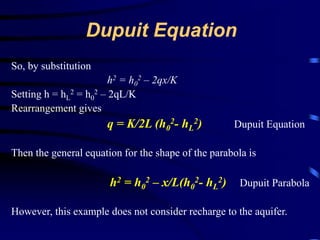
Downloaded 148 times


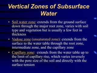


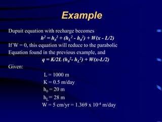
![Example
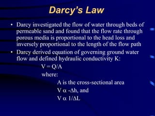
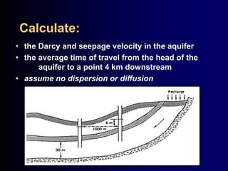
For discharge into River 1, set x = 0 m
q = K/2L (h0
2- hL
2) + W(0-L/2)
= [(0.5 m/day)/(2)(1000 m)] (202 m2 – 18 m2 ) +
(1.369 x 10⁻⁴ m/day)(-1000 m / 2)
q = – 0.05 m2 /day
The negative sign indicates that flow is in the opposite direction
From the x direction. Therefore,
q = 0.05 m2 /day into river 1](https://image.slidesharecdn.com/ch02intro-141107153727-conversion-gate01/85/Ch02intro-47-320.jpg)
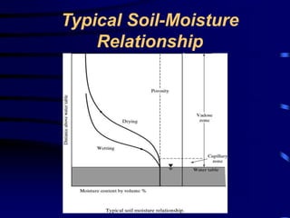
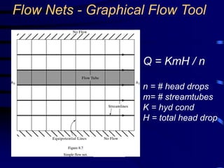
![Example
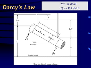
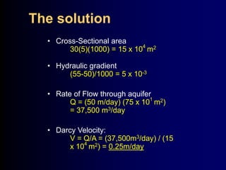
For discharge into River 2, set x = L = 1000 m:
q = K/2L (h0
2- hL
2) + W(L-L/2)
= [(0.5 m/day)/(2)(1000 m)] (202 m2 – 18 m2 ) +
(1.369 x 10⁻⁴ m/day)(1000 m –(1000 m / 2))
q = 0.087 m2/day into River 2
By setting q = 0 at the divide and solving for xd, the
water divide is located 361.2 m from the edge of
River 1 and is 20.9 m high](https://image.slidesharecdn.com/ch02intro-141107153727-conversion-gate01/85/Ch02intro-48-320.jpg)
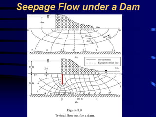

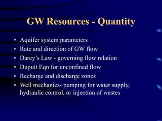
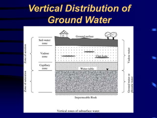
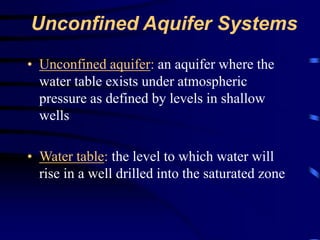
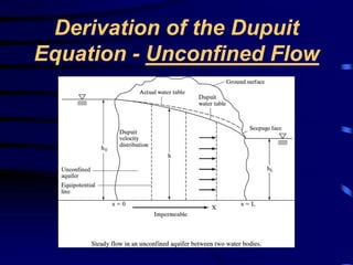
This document provides an overview of groundwater hydrology and aquifer systems. It discusses key topics such as: - Aquifer parameters like porosity, hydraulic conductivity, and storage coefficients. - Governing equations for groundwater flow including Darcy's Law and the Dupuit equation for unconfined flow. - Vertical zones of subsurface water and soil moisture relationships. - Characteristics of confined and unconfined aquifers. - Flow nets as a graphical tool for analyzing groundwater flow patterns. The document serves as an introduction to analyzing groundwater resources and flow using fundamental hydrogeological principles.


![09. Silt Theories [Kennedy's Theory].pdf](https://cdn.slidesharecdn.com/ss_thumbnails/09-230714062702-13879994-thumbnail.jpg?width=640&height=640&fit=bounds)