This is created by Dr.Krishna Achuta Rao, Centre for Atmospheric Sciences, IIT-Delhi, for taking CDAT class. It's under Creative Common License 3.0

1. Introduction to Arrays, Variables

2. Preview
• What is an array and the NumPy package
– Creating arrays
– Array indexing
– Array inquiry
– Array manipulation
– Array operations
• What is (in) CDAT?
– Masked variables, axes
– Brief tour of vcdat

3. What is an array and the NumPy package
• An array is like a list except:
– All elements are of the same type, so operations with
arrays are much faster.
– Multi‐dimensional arrays are more clearly supported.
– Array operations are supported.
• NumPy is the standard array package in Python.
(There are others, but the community has now
converged on NumPy.)
• To utilize NumPy's functions and attributes, you
import the package numpy.

4. Creating arrays
• Use the array function on a list:
import numpy
a = numpy.array([[2, 3, -5],[21, -2, 1]])
• The array function will match the array type to
the contents of the list.
• To force a certain numerical type for the array,
set the dtype keyword to a type code:
a = numpy.array([[2, 3, -5],[21, -2, 1]],
dtype='d')

5. Creating arrays (cont.)
• Some common typecodes:
– 'd': Double precision floating
– 'f': Single precision floating
– 'i': Short integer
– 'l': Long integer
• To create an array of a given shape filled with zeros,
use the zeros function (with dtype being optional):
a = numpy.zeros((3,2), dtype='d')
• To create an array the same as range, use the
arange function (again dtype is optional):
a = numpy.arange(10)

6. Array indexing
• Like lists, element addresses start with zero, so the first
element of 1‐D array a is a[0], the second is a[1], etc.
• Like lists, you can reference elements starting from the end,
e.g., element a[-1] is the last element in a 1‐D array.
• Slicing an array:
– Element addresses in a range are separated by a colon.
– The lower limit is inclusive, and the upper limit is exclusive.
• Type the following in the Python interpreter:
import numpy
a = numpy.array([2, 3.2, 5.5, -6.4, -2.2, 2.4])
• What is a[1] equal to? a[1:4]? Share your answers
with your neighbor.

7. Array indexing (cont.)
• For multi‐dimensional arrays, indexing between different
dimensions is separated by commas.
• The fastest varying dimension is the last index. Thus, a 2‐D array is
indexed [row, col].
• To specify all elements in a dimension, use a colon by itself for the
dimension.
• Type the following in the Python interpreter:
import numpy
a = numpy.array([[2, 3.2, 5.5, -6.4, -2.2, 2.4],
[1, 22, 4, 0.1, 5.3, -9],
[3, 1, 2.1, 21, 1.1, -2]])
• What is a[1,2] equal to? a[1,:]? a[1:4,0]? What is
a[1:4,0:2]? (Why are there no errors?) Share your answers
with your neighbor.

8. Array inquiry
• Some information about arrays comes through functions on
the array, others through attributes attached to the array.
• For this and the next slide, assume a and b are numpy
arrays.
• Shape of the array: numpy.shape(a)
• Rank of the array: numpy.rank(a)
• Number of elements in the array (do not use len):
numpy.size(a)
• Typecode of the array: a.dtype.char
• Try these commands out in your interpreter on an array you
already created and see if you get what you expect.

9. Array manipulation
• Reshape the array: numpy.reshape(a, (2,3))
• Transpose the array: numpy.transpose(a)
• Flatten the array into a 1‐D array: numpy.ravel(a)
• Repeat array elements: numpy.repeat(a,3)
• Convert array a to another type:
b = a.astype('f')
where the argument is the typecode for b.
• Try these commands out in your interpreter on an
array you already created and see if you get what you
expect.

10. Array operations: Method 1 (loops)
• Example: Multiply two arrays together, element‐by‐element:
import numpy
shape_a = numpy.shape(a)
product = numpy.zeros(shape_a, dtype='f')
a = numpy.array([[2, 3.2, 5.5, -6.4],
[3, 1, 2.1, 21]])
b = numpy.array([[4, 1.2, -4, 9.1],
[6, 21, 1.5, -27]])
for i in xrange(shape_a[0]):
for j in xrange(shape_a[1]):
product[i,j] = a[i,j] * b[i,j]
• Note the use of xrange (which is like range, but provides only
one element of the list at a time) to create a list of indices.
• Loops are relatively slow.
• What if the two arrays do not have the same shape?

11. Array operations: Method 2 (array syntax)
• Example: Multiply two arrays together, element‐by‐element:
import numpy
a = numpy.array([[2, 3.2, 5.5, -6.4],
[3, 1, 2.1, 21]])
b = numpy.array([[4, 1.2, -4, 9.1],
[6, 21, 1.5, -27]])
product = a * b
• Arithmetic operators are automatically defined to act element‐wise
when operands are NumPy arrays. (Operators have function
equivalents, e.g., product, add, etc.)
• Output array automatically created.
• Operand shapes are automatically checked for compatibility.
• You do not need to know the rank of the arrays ahead of time.
• Faster than loops.

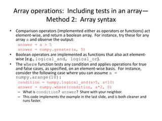
12. Array operations: Including tests in an array—
Method 1: Loops
• Often times, you will want to do calculations on an array that
involves conditionals.
• You could implement this in a loop. Say you have a 2‐D array a and
you want to return an array answer which is double the value
when the element in a is greater than 5 and less than 10, and
output zero when it is not. Here's the code:
answer = numpy.zeros(numpy.shape(a), dtype='f')
for i in xrange(numpy.shape(a)[0]):
for j in xrange(numpy.shape(a)[1]):
if (a[i,j] > 5) and (a[i,j] < 10):
answer[i,j] = a[i,j] * b[i,j]
else:
pass
– The pass command is used when you have an option where you
don't want to do anything.
– Again, loops are slow, and the if statement makes it even slower.

13. Array operations: Including tests in an array—
Method 2: Array syntax
• Comparison operators (implemented either as operators or functions) act
element‐wise, and return a boolean array. For instance, try these for any
array a and observe the output:
answer = a > 5
answer = numpy.greater(a, 5)
• Boolean operators are implemented as functions that also act element‐
wise (e.g., logical_and, logical_or).
• The where function tests any condition and applies operations for true
and false cases, as specified, on an element‐wise basis. For instance,
consider the following case where you can assume a =
numpy.arange(10):
condition = numpy.logical_and(a>5, a<10)
answer = numpy.where(condition, a*2, 0)
– What is condition? answer? Share with your neighbor.
– This code implements the example in the last slide, and is both cleaner and
runs faster.

14. Array operations: Including tests in an array—
Method 2: Array syntax (cont.)
• You can also accomplish what the where function does in the
previous slide by taking advantage of how arithmetic operations on
boolean arrays treat True as 1 and False as 0.
• By using multiplication and addition, the boolean values become
selectors. For instance:
condition = numpy.logical_and(a>5, a<10)
answer = ((a*2)*condition) +
(0*numpy.logical_not(condition))
• This method is also faster than loops.
• Try comparing the relative speeds of these different ways of
applying tests to an array. The time module has a function time
so time.time() returns the current system time relative to the
Epoch. (This is an exercise that is available online.)

15. Array operations: Additional functions
• Basic mathematical functions: sin, exp,
interp, etc.
• Basic statistical functions: correlate,
histogram, hamming, fft, etc.
• NumPy has a lot of stuff! Use
help(numpy), as well as
help(numpy.x), where x is the name of a
function, to get more information.

16. Exercise 1: Reading a multi‐column text
file (simple case)
• For the file two‐col_rad_sine.txt in files, write
code to read the two columns of data into two
arrays, one for angle in radians (column 1) and
the other for the sine of the angle (column 2).
• The two columns are separated by tabs. The
file's newline character is just 'n' (though
this isn't something you'll need to know to do
the exercise).

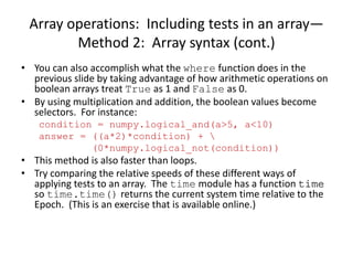
17. Exercise 1: Reading a multi‐column text
file (solution for simple case)
import numpy
DATAPATH = ‘/CAS_OBS/sample_cdat_data/’
fileobj=open(DATAPATH + 'two-col_rad_sine.txt', 'r')
data_str = fileobj.readlines()
fileobj.close()
radians = numpy.array(len(data_str), 'f')
sines = numpy.array(len(data_str), 'f')
for i in xrange(len(data_str)):
split_istr = data_str[i].split('t')
radians[i] = float(split_istr[0])
sines[i] = float(split_istr[1])

18. Exercise 2 (Homework): Reading
formatted data
• In the directory
/CAS_OBS/sample_cdat_data/ you
will see the following files
– REGIONRF.TXT (a data file with rainfall data for
India)
– test_FortranFormat.py
• Look at the python program and try to
understand what it does and do the exercise
given in it.

19. What is CDAT?
• Designed for climate science data, CDAT was first released in 1997
• Based on the object‐oriented Python computer language
• Added Packages that are useful to the climate community and other
geophysical sciences
– Climate Data Management System (CDMS)
– NumPy / Masked Array / Metadata
– Visualization (VCS, IaGraphics, Xmgrace, Matplotlib, VTK, Visus, etc.)
– Graphical User Interface (VCDAT)
– XML representation (CDML/NcML) for data sets
• One environment from start to finish
• Integrated with other packages (i.e., LAS, OPeNDAP, ESG, etc.)
• Community Software (BSD open source license)
• URL: http://www‐pcmdi.llnl.gov/software‐portal (CDAT Plone site)

20. CDMS: cdms2
• Best way to ingest and write NetCDF‐CF, HDF, Grib, PP,
DRS, etc., data!
• Opening a file for reading
import cdms2
f=cdms2.open(file_name)
– It will open an existing file protected against writing
• Opening a new file for writing
f=cdms2.open(file_name,’w’)
– It will create a new file even if it already exists
• Opening an existing file for writing
f=cdms2.open(file_name,’r+’) # or ‘a’
– It will open an existing file ready for writing or reading

21. A NetCDF example and VCDAT
• Change directory to the following directory
cd /CAS_OBS/mo/sst/HadISST/
• Check the contents of the netcdf file
ncdump sst_HadISST_Climatology_1961-1990.nc | more
• Start vcdat
vcdat &
• Note what happens when you click on the “file”
pulldown arrow
• Select variable “sst”
• Press “plot”

22. Exercise 2: Opening a NetCDF file
import cdms2
DATAPATH = ‘/CAS_OBS/mo/sst/HadISST/’
f = cdms2.open(DATAPATH + ‘sst_HadISST_Climatology_1961-1990.nc’)
# You can query the file
f.listvariables()
# You can “access” the data through file variable
x = f[‘sst’]
# or read all of it into memory
y = f(‘sst’)
# You can get some information about the variables by
x.info()
y.info()
# You can also find out what class the object x or y belong to
print x.__class__
# Close the file
f.close()

23. CDMS: cmds2 (cont.)
• Multiple way to retrieve data
– All of it, omitted dimensions are retrieved entirely
s=f(‘var’)
– Specifying dimension type and values
S=f(‘var’, time=(time1,time2))
• Known dimension types: time, level, latitude, longitude (t,z,y,x)
– Dimension names and values
S=f(‘var’,dimname1=(val1,val2))
– Sometimes indices are more useful than actual values
S=f(‘var’,time=slice(index1,index2,step))

24. cdtime module
• Import the cdtime module
import cdtime
• Relative time
r = cdtime.reltime(19, “days since 2011-5-1”)
• Component time
c = cdtime.comptime(2011, 5, 20)
• You can interchange between component and
relative time
c.torel(“days since 2011-1-1”)
r.tocomp()

25. Arrays, Masked Arrays and Masked
Variables
array numpy
array mask
numpy.ma
+
array mask domain metadata MV2
+ + + id,units,…

26. Arrays, Masked Arrays and Masked
Variables
>>> a=numpy.array([[1.,2.],[3,4],[5,6]])
>>> a.shape
(3, 2)
>>> a[0]
array([ 1., 2.])
>>> numpy.ma.masked_greater(a,4)
masked_array(data =
[[1.0 2.0]
[3.0 4.0]
[‐‐ ‐‐]],
mask =
[[False False]
[False False]
[ True True]],
fill_value = 1e+20)
>>>b = MV2.masked_greater(a,4)
>>> b.info()
*** Description of Slab variable_3 ***
id: variable_3
shape: (3, 2)
filename:
missing_value: 1e+20
comments:
grid_name: N/A
grid_type: N/A
time_statistic:
long_name:
units:
No grid present.
** Dimension 1 **
id: axis_0
Length: 3
First: 0.0
Last: 2.0
Python id: 0x2729450
** Dimension 2 **
id: axis_1
Length: 2
First: 0.0
Last: 1.0
Python id: 0x27292f0
*** End of description for variable_3 ***
These values
are now
MASKED
(average
would ignore
them)
Additional info
such as
metadata
and axes

27. Summary
• Take advantage of NumPy's array syntax to
make operations with arrays both faster and
more flexible (i.e., act on arrays of arbitrary
rank).
• Use any one of a number of Python packages
(e.g., CDAT, PyNIO, pysclint, PyTables,
ScientificPython) to handle netCDF, HDF, etc.
files.

28. Acknowledgments
Original presentation by Dr. Johnny Lin (Physics
Department, North Park University, Chicago,
Illinois).
Author email: johnny@johnny‐lin.com. Presented
as part of an American Meteorological Society short
course in Seattle, Wash. on January 22, 2011. This
work is licensed under a Creative Commons
Attribution‐NonCommercial‐ShareAlike 3.0 United
States License.