This document presents a discrete valuation methodology for swing options using a forest model approach. It develops numerical implementations of swing options on one-factor and two-factor mean-reverting underlying processes using binomial trees. It establishes convergence via finite difference methods and considers qualitative properties and sensitivity analysis. The methodology values swing options as a system of coupled European options and allows for various discrete models of the underlying process.

![2 ALI LARI-LAVASSANI, MOHAMADREZA SIMCHI, AND ANTONY WARE
is straightforward but leads to challenging computational problems due to high
dimensionality. One promising avenue would be to investigate numerical imple-
mentation on parallel computer. We do however allow the single underlying asset
to follow a multi-factor stochastic process. A distinctive characterization of the
methodology developed here is its abstract and general nature, which makes it ap-
plicable to any discrete modeling of the underlying asset, in particular binomial or
trinomial trees, or indeed trees with any number of branching jumps. This abstract
setting lends itself to a European style of exercise of the swing rights. We fully
develop numerical implementations of swing options on mean-reverting underlying
processes via binomial trees.
The paper is written in a self contained manner and full arguments are presented
to the extent possible. It is organized as follows: Section 2 discusses some classical
examples of one- and two-factor mean-reverting linear stochastic differential equa-
tions. These model energy price or interest rate processes, and throughout this
work, they will be used to illustrate the methods and results. Section 3 presents a
general abstract look at discrete modeling of stochastic processes. Section 4 inves-
tigates numerical implementations of mean-reverting processes on binomial trees.
Section 5 describes a general swing option contract. Section 6 develops a mathe-
matical model for the swing option via a forest methodology. Section 7 is devoted
to numerical investigation of convergence, hedge parameters and comparison with
a basket of American options. Section 8 proves the convergence of the binomial
tree swing option valuation, showing that the upper bound on the error is inversely
proportional to the number of time steps in the tree.
2. Underlying Processes and Applications to Energy Models
The general setting for swing options developed in Section 6 is quite abstract and
applies to all discrete processes. To make ideas more transparent we first introduce
in this section one- and two-factor models historically used for short term interest
rates, and which are now finding applications in the energy commodity markets
as in [S, 1998], [P, 1997], [HR, 1998], [JRT, 1998]. When using these models to
price options, it is implicitly assumed that they reflect the risk neutralized price
processes, perhaps via the incorporation of a model of the cost-of-carry or the
market-price-of-risk functions, see [H, 1999]. This will be the working assumption
for the remainder of this paper.
A general diffusion one-factor model is:
dSt = µ(St, t)dt + σ(St, t)dZt,(2.1)
where µ and σ are C2
differentiable and satisfy the usual linear growth conditions
to guarantee the existence of solutions of the above stochastic differential equation
(see [KP, 1999] Theorem 4.5.3, p. 131), and dZt is a standard Brownian motion,
E(dZt) = 0, and E((dZt)2
) = dt. We will consider two classical particular cases:
dSt = µSt dt + σSt dZt(2.2)
dSt = α(L − St) dt + σSt dZt,(2.3)
where µ, α, σ and L are constants. The following system of stochastic linear
differential equations is a possible two-factor model for energy and commodity spot](https://image.slidesharecdn.com/2e137caa-c106-45e4-b98c-2c28cf277cf9-170125135748/85/SwingOptions-2-320.jpg)
![A DISCRETE VALUATION OF SWING OPTION 3
price processes:
dSt = α(Lt − St) dt + σSt dZt
dLt = µ Lt dt + ξLt dWt,
(2.4)
where α, µ, σ and ξ are constants and dZt and dWt are uncorrelated standard
Brownian motions.
Ignoring the stochastic parts in the mean-reverting equations (2.3) and (2.4)
yields the deterministic differential equations governing the time evolution of the
mean of each process:
dE(St)
dt
= α(L − E(St))(2.5)
d
dt
E(St)
E(Lt)
=
−α α
0 µ
E(St)
E(Lt)
.(2.6)
We shall establish that the orbits associated with the E(Lt) equations are at-
tracting invariant spaces for the flows of these deterministic stochastic differential
equations. This justifies the use of the terms long-run mean and mean-reverting.
For more on the notions of dynamical systems introduced in the next Proposition
and its proof we refer to [R, 1995] Chapter 5.
Proposition 1. For the process St, given by (2.3), L is the stable equilibrium of
the hyperbolic differential equation governing (2.5) if α > 0. For the process St,
given by (2.4), the orbit of E(Lt) is the unstable or stable manifold of the hyperbolic
differential equation (2.6). This is the unstable manifold when α > 0, and µ > 0,
which is the case for the financial applications we are considering.
Proof. Let S0 be the value of St at t = t0. E(St) = L is the equilibrium of (2.5).
Since the eigenvalue −α < 0, stability follows. Therefore as t −→ ∞, the solution
curves of E(St) decay exponentially to L. Denote the two-by-two matrix of (2.6) by
A, and the value of Lt at t = t0 by L0. This system is hyperbolic since the real part
of the eigenvalues −α and µ of A are nonzero. Furthermore, the equilibrium at the
origin is a saddle since −α < 0, and µ > 0. The stable and unstable manifolds of
this hyperbolic equilibrium are the corresponding eigenspaces and, since the system
is linear, they are global [R, 1995] Theorem 6.1, p. 111. They are respectively the
lines, {(1, 0) e−α (t−t0)
, t ∈ R} and {( α
µ+α , 1) L0 eµ (t−t0)
, t ∈ R} in the phase space
(E(St), E(Lt)). The solution to the above linear system is given by (see [R, 1995]
Proposition 3.1, p. 97)
E(St)
E(Lt)
= e(t−t0)A S0
L0
=
S0e−α(t−t0)
+ α
α+µ L0(eµ(t−t0)
− e−α(t−t0)
)
L0eµ(t−t0)
which can be decomposed in term of the direct sum of the stable and unstable
manifolds as
S0 −
α
α + µ
L0 e−α(t−t0) 1
0
+ L0eµ(t−t0)
α
α+µ
1
.
Dynamically speaking, in the phase space, any trajectory t −→ (E(St), E(Lt)), off
the stable or unstable manifolds, tends in forward time as t −→ ∞, to L0eµ(t−t0) α
µ+α , 1
which is the unstable manifold.](https://image.slidesharecdn.com/2e137caa-c106-45e4-b98c-2c28cf277cf9-170125135748/85/SwingOptions-3-320.jpg)
![4 ALI LARI-LAVASSANI, MOHAMADREZA SIMCHI, AND ANTONY WARE
Note that we used the notation E(St) to denote the conditional expectation
E(St|St0
)|t. We next gather and present results on the first moments of the above
processes:
Proposition 2. a) Consider the process, dSt = (µSt + b)dt + σSt dZt over the
time interval [ti, tk], where µ, b and σ are constants and let Sti = Si. We make the
generic non-degeneracy assumptions:
(H1) σ2
+ µ = 0, 2µ + σ2
= 0 and µ = 0.
Then the first and second moments of St are given by:
E(St|Si)|tk
= −
b
µ
+ (Si +
b
µ
)eµ(tk−ti)
,
E(S2
t |Si)|tk
= c e(2µ+σ2
)(tk−ti)
−
2b(Si + b
µ )
σ2 + µ
eµ(tk−ti)
+
2b2
µ(2µ + σ2)
,
where
c = Si
2
−
2b(Si + b
µ )
σ2 + µ
+
2b2
µ(2µ + σ2)
.
b) Consider the process given by (2.4) over the time interval [ti, tk], and let Sti
= Si,
Lti
= Li. We make the generic non-degeneracy assumptions:
(H2) µ + α − σ2
= 0 = (2µ + ξ2
− σ2
+ 2α) = 0 = (µ + ξ2
+ α) = 0
Then the first and second moments are given by:
E(St|Si)|tk
= Sie−α(tk−ti)
+
α
α + µ
Li(eµ(tk−ti)
− e−α(tk−ti)
),
E(Lt|Li)|tk
= Lieµ(tk−ti)
,
E((St, St)|Si)|tk
= S2
i ϕ1(tk − ti) +
2α
Ψ
SiLi(ϕ1(tk − ti) − ϕ2(tk − ti))
+2α2
L2
i (
−ϕ1(tk − ti)
ΨΓ
+
ϕ2(tk − ti)
ΨΘ
+
ϕ3(tk − ti)
ΘΓ
),
E((St, Lt)|(Si, Li))|tk
= ϕ2(tk − ti)SiLi +
α
Θ
L2
i (ϕ3(tk − ti) − ϕ2(tk − ti))
E((Lt, Lt)|Li)|tk
= L2
i ϕ3(tk − ti),
where ϕ1(t) = e(σ2
−2α)(tk−ti)
, ϕ2(t) = e(µ−α)(tk−ti)
, ϕ3(t) = e(2µ+ξ2
)(tk−ti)
, Ψ =
−µ − α + σ2
, Θ = µ + ξ2
+ α, and Γ = 2µ + ξ2
− σ2
+ 2α.
Remark 2.1. By generic is meant that in the parameter space R{σ, µ} or
R{σ, µ, α}, the set of values satisfying (H1) or (H2) is open and dense. See [HS,
1974] p 154. From a mathematical modeling point of view, it suffices to only study
generic models since any model can be made generic via a small perturbation.
Proof. The differential equations governing time evolution of E(St) and E(S2
t ) are
give in [KP, 1999] p. 113, see also, [G, 1997] p. 113. For the case at hand, they
become,
d
dt
(E(St)) = µE(St) + b
d
dt
(E(S2
t ) = (2µ + σ2
) E(S2
t ) + 2bE(St).
Then a simple integration yields the result. The system of ordinary differential
equations governing the time evolution of the first and second moments of St and](https://image.slidesharecdn.com/2e137caa-c106-45e4-b98c-2c28cf277cf9-170125135748/85/SwingOptions-4-320.jpg)
![A DISCRETE VALUATION OF SWING OPTION 5
Lt are quoted in general in [KP, 1999] p. 152. For the first moments E(St) and
E(Lt), these equations are (2.6), and they were solved in the proof of Proposition
1. The equations for the second moments become:
d
dt
E(St, St)
E(St, Lt)
E(Lt, Lt)
=
(σ2
− 2α) 2α 0
0 (µ − α) α
0 0 (ξ2
+ 2µ)
E(St, St)
E(St, Lt)
E(Lt, Lt)
.
Denoting the above three-by-three matrix by B, the solution to this system is
given by
E(St, St)
E(St, Lt)
E(Lt, Lt)
= e(tk−ti)B
S2
i
SiLi
L2
i
.
The computation of e(tk−ti)B
is routine in an eigenbasis, see [HS, 1974] chapter 7,
or can be carried out in one operation in the symbolic language Maple.
3. An Abstract Approach to Discrete Processes
Traditionally in mathematical finance literature various discrete modeling of sto-
chastic processes under the guise of binomial or trinomial trees (and beyond) have
been introduced. A single abstract unifying framework can be developed for all
these trees. Consider a single or multi-factor stochastic process St modeled dis-
cretely over some time interval. At each time step i, the possible states of the
world are given by finitely many vectors S(i)
= (S
(i)
j ), where j is in a finite index
set J(i)
. Note that we are not restricting ourselves to one-dimensional models by
this notation. The state vector S(i)
can incorporate the values of the underlying
asset as well as secondary factors in the multi-factor case. As time flows from the
time step i to i + 1, the discrete node S
(i)
j can go to any S
(i+1)
j
, j ∈ J(i+1)
. What
determines the discrete process is a transition probability matrix P(i)
= (P
(i)
j,j ),
so that the element P
(i)
j,j represents the probability of S
(i)
j going to S
(i+1)
j
. The
number of rows in P(i)
is the cardinal of J(i)
, and the number of columns is the
cardinal of J(i+1)
; and for all j ∈ J(i)
,
j ∈J(i+1)
P
(i)
j,j = 1.
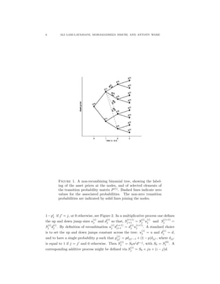
Example 3.1. A one-factor non-recombining binomial discrete stochastic pro-
cess is S(i)
= (S
(i)
j ) with j ∈ J(i)
= 1, . . . , 2i
. The transition probabilities are
given for every i by a vector (pi
j), j ∈ J(i)
, such that P
(i)
j,j is defined to be pi
j
if j = 2j, 1 − pi
j if j = 2j − 1, or 0 otherwise, as depicted in Figure 1. The
dashed lines in that figure represent prohibited connections which are ruled out by
setting their corresponding probabilities equal to zero. In a multiplicative process
one defines the up and down jump sizes u
(i)
j and d
(i)
j such that, S
(i+1)
2j = S
(i)
j u
(i)
j
and S
(i+1)
2j−1 = S
(i)
j d
(i)
j . We note that this tree is not numerically efficient since the
number of nodes grows exponentially with time.
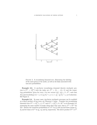
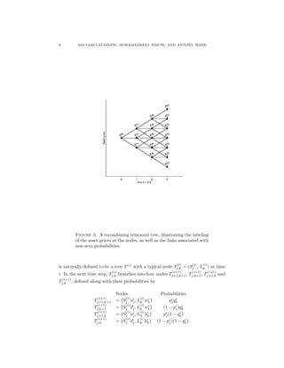
Example 3.2. A one-factor recombining binomial discrete stochastic process is
S(i)
= (S
(i)
j ) with j ∈ J(i)
= {1, . . . , i + 1}. The transition probabilities, are given
for every i by a vector (pi
j), j ∈ J(i)
, such that P
(i)
j,j is defined to be pi
j if j = j +1,](https://image.slidesharecdn.com/2e137caa-c106-45e4-b98c-2c28cf277cf9-170125135748/85/SwingOptions-5-320.jpg)
![A DISCRETE VALUATION OF SWING OPTION 9
4. Numerical Implementations
In this section we derive formulae for numerical implementations of various under-
lying processes discussed in Section 2 in terms of the multiplicative recombining
binomial trees of Section 3. We first discuss the general, equation (2.1) and deduce
the cases of log-normal and one factor mean-reverting processes as an application.
We next show that up to the first order approximation, the two-factor model (2.4)
can be discretized as a direct product of the two one-factor trees above.
Consider the discrete binomial process S(i)
wherein the value of the process at
the time step i, given by S
(i)
j , can undergo an up jump to S
(i+1)
j +1 = S
(i)
j ui
j with
the probability pi
j, or a down jump to S
(i+1)
j = S
(i)
j di
j. Note that this situation
is general enough to encompass both Example 1 and 2 of Section 3, and to also
include the possibilities of multiple jumps. To approximate a continuous process,
we match the first and the second moments of the discontinuous process on the tree
with those of the continuous process over time intervals of length ∆t.
Proposition 3. Consider the continuous process dSt = µ(St, t)dt + σ(St, t)dZt as
in (2.1), and the recombining binomial tree (S
(i)
j ) = S(i)
described above. Assume
that at t = ti, Sti = S
(i)
j . Over the time interval [ti, ti + ∆t], we denote the
conditional expectations of the continuous process by E(St|Sti )|ti+∆t, and that of
the discrete process by Ed(S(i)
|S
(i)
j )|ti+∆t.
Matching the first and second moments of these two processes results in the
binomial tree specified by:
pi
j =
A(Sti , ∆t) − di
j
ui
j − di
j
, ui
j = ecosh−1
(θ)
, di
j = 1/ui
j(4.1)
where,
A(Sti , ∆t) := E(St|Sti )|ti+∆t/S
(i)
j ,
B(Sti
, ∆t) := E(S2
t |Sti
)|ti+∆t/(S
(i)
j )2
,
θ(Sti
, ∆t) :=
1 + B(Sti
, ∆t)
2A(Sti , ∆t)
Remark 2.2. This general result applies to all binomial approximation schemes.
Some classical particular cases are discussed in [K,1998] Chapter 5.1.
Proof. Using the definition of Ed(.|.), the matching equations become
Ed(S(i)
|S
(i)
j )|ti+∆t : = pi
jS
(i+1)
j +1 + (1 − pi
j)S
(i+1)
j = E(St|Sti
)|ti+∆t
Ed((S(i)
)2
|S
(i)
j )|ti+∆t : = pi
j(S
(i+1)
j +1 )2
+ (1 − pi
j)(S
(i+1)
j )2
= E(S2
t |Sti
)|ti+∆t
Since S
(i+1)
j +1 = S
(i)
j ui
j and S
(i+1)
j = S
(i)
j di
j, the above equations reduce to
pi
jui
j + (1 − pi
j)di
j = A(Sti
, ∆t)(4.2)
pi
jui2
j + (1 − pi
j)di2
j = B(Sti
, ∆t)](https://image.slidesharecdn.com/2e137caa-c106-45e4-b98c-2c28cf277cf9-170125135748/85/SwingOptions-9-320.jpg)
![10 ALI LARI-LAVASSANI, MOHAMADREZA SIMCHI, AND ANTONY WARE
where A(Sti
, ∆t) := E(St|Sti
)|ti+∆t/Si
j and B(Sti
, ∆t) := E(S2
t |Sti
)|ti+∆t/Si2
j .
Solving for pi
j results in pi
j =
A(Sti
,∆t)−di
j
ui
j −di
j
. To remove an extra degree of free-
dom in these equations we assume that di
j = 1/ui
j, then substituting pi
j into the
second equation and solving gives ui
j +di
j =
1+B(Sti
,∆t)
A(Sti
,∆t) , which yields the result.
Remark 2.3. One should note1
that 0 ≤ pi
j ≤ 1. Moreover, although the
above values for ui
j and di
j match (4.2) precisely, in general they will not result in
a recombining tree. In practice, for every particular choice of µ(St, t) and σ(St, t)
in Equation (2.1) appropriate approximations must be chosen to ensure numerical
feasibility as in the following theorem.
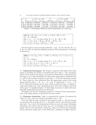
Theorem 1. a) Consider the linear stochastic differential equation
dSt = (µSt + b)dt + σStdZt
with constant coefficients over the time interval [t0, T]. Let S(i)
= (S
(i)
j ) be a
recombining binomial tree as described in Example 3.2, with time step ∆t. Suppose
there exists a lower bound Smin = 0 such that S
(i)
j > Smin for all i, j. Matching
the first and second moments of S(i)
= (S
(i)
j ) with those of St, up to order ∆t and
for Si
j above Smin, results in
pi
j =
1
2
+
µ + b/S
(i)
j − σ2
/2
2σ
√
∆t , ui
j = eσ
√
∆t
, di
j = 1/ui
j.
b) Without assuming a lower bound Smin, the log-normal process dSt = µSt dt+σS
dZt can be discretized by a recombining binomial tree with
pi
j =
1
2
+
µ − σ2
/2
2σ
√
∆t , ui
j = eσ
√
∆t
, di
j = 1/ui
j.
1To see why this is so, note first that the definitions of A(Sti , ∆t) and B(Sti , ∆t) as normalized
expectations of S(t) and (S(t))2 respectively imply (dropping extraneous notation) that
B ≥ A2
.
One immediate consequence of this is that
θ =
1 + B
2A
≥
1 + A2
2A
= 1 +
(A − 1)2
2A
≥ 1.
A second consequence is that
2Aθ = 1 + B ≥ 1 + A2
,
so that
1 + A2
− 2Aθ ≤ 0.
By adding θ2 − 1 to both sides we obtain
(A − θ)2
≤ θ2
− 1.
It follows now that
θ − θ2 − 1 ≤ A ≤ θ + θ2 − 1.
Noting that cosh−1
θ = ln(θ +
√
θ2 − 1) we see that we have
d ≤ A ≤ u.
The required result now follows directly from the definition of p.](https://image.slidesharecdn.com/2e137caa-c106-45e4-b98c-2c28cf277cf9-170125135748/85/SwingOptions-10-320.jpg)
![12 ALI LARI-LAVASSANI, MOHAMADREZA SIMCHI, AND ANTONY WARE
Theorem 2. Consider the system of linear stochastic differential equations (2.4)
over the time interval [t0, T],
dSt = α(Lt − St) dt + σSt dZt
dLt = µLt dt + ξLt dWt,
a) Over any interval [ti, ti + ∆t] ⊂ [t0, T], the processes St and Lt will remain
uncorrelated up to the order O(∆t, Sti , Lti ).
b) Let S(i)
= (S
(i)
j ) and L(i)
= (L
(i)
k ) be recombining binomial trees as described
in Example 3.2, with time step ∆t. Suppose there exist lower and upper bounds
Smin = 0, respectively Lmax < ∞ such that S
(i)
j > Smin and L
(i)
k < Lmax for all
i, j, k. Then, away from Smin and Lmax, matching the first and second moments
of S(i)
, respectively L(i)
with those of St, respectively Lt, and up to order ∆t results
in
L(i)
: qi
k =
1
2
+
µ − ξ2
2ξ
√
∆t , wi
k = eξ
√
∆t
, hi
k = 1/wi
k.
S(i)
: pi
j =
1
2
+ (α
L
(i)
k /S
(i)
j − 1
2σ
−
σ
4
)
√
∆t , ui
j = eσ
√
∆t
, di
j = 1/ui
j.
The above system can be discretized as a direct product of the two trees S(i)
×L(i)
described in Example 3.4.
Proof. a) Assume that at t = ti the value of St is S
(i)
j and that the value of Lt is
L
(i)
k . A first order approximation of the results obtained in Proposition 2 part b)
yields
E(St|S
(i)
j )|ti+∆t = S
(i)
j + α(L
(i)
k − S
(i)
j )∆t + O(∆t2
, Sti , Lti )
E(Lt|L
(i)
k )|ti+∆t = L
(i)
k + µL
(i)
k ∆t + O(∆t2
, Lti
)
and
E((St, St)|S
(i)
j )|ti = (S
(i)
j )2
+ ((σ2
− 2α)(S
(i)
j )2
+ 2αS
(i)
j L
(i)
k )∆t + O(∆t2
, Sti , Lti )
E((St, Lt)|(S
(i)
j , L
(i)
k ))|ti
= S
(i)
j L
(i)
k + ((µ − α)S
(i)
j L
(i)
k + α(L
(i)
k )2
)∆t + O(∆t2
, Sti
, Lti
)
E((Lt, Lt)|L
(i)
k )|ti
= (L
(i)
k )2
+ (ξ2
+ 2µ)∆t + O(∆t2
, Lti
).
Therefore, up to O(∆t, Sti , Lti ),
Cov(St, Lt)|ti
= E((St, Lt)|(S
(i)
j , L
(i)
k ))|ti
− E(St|S
(i)
j )|ti+∆t E(Lt|L
(i)
k )|ti+∆t = 0
and hence at (S
(i)
j , L
(i)
k ) and up to O(∆t, Sti , Lti ) the processes St and Lt will
remain uncorrelated over [ti, ti + ∆t].
b) By part a) at each (S
(i)
j , L
(i)
k ) the two processes St and Lt remain uncorrelated
over [ti, ti + ∆t]. Therefore at such a point and over [ti, ti + ∆t], St and Lt can
be approximated by independent binomial trees, and hence (2.4) can in turn be
approximated by the direct product of these two trees over the same time interval.
Since L is a log-normal process, part b) of Theorem 1 yields the tree L(i)
. Note that,
at (S
(i)
j , L
(i)
k ), St follows a one-factor mean-reverting process (2.3) with L = L
(i)
k .](https://image.slidesharecdn.com/2e137caa-c106-45e4-b98c-2c28cf277cf9-170125135748/85/SwingOptions-12-320.jpg)
![A DISCRETE VALUATION OF SWING OPTION 13
Therefore from Theorem 1 we have
A(Sti
, ∆t) =
L
(i)
k
S
(i)
j
+ (1 −
L
(i)
k
S
(i)
j
) e−α∆t
B(Sti
, ∆t) =
c
(S
(i)
j )2
e(σ2
−2α)∆t
−
2αL
(i)
k (Si
j − L
(i)
k )
(σ2 − α)(S
(i)
j )2
e−α∆t
−
2αL
(i)
k
2
(σ2 − 2α)(S
(i)
j )
2 .
Note that since Smin and Lmax exist
L
(i)
k
S
(i)
j
is bounded. Therefore A and B can be
uniformly expanded in Taylor series, as in Theorem 1. Hence the tree of S follows
from part c) of Theorem 1.
5. A General Swing Contract
We begin by introducing the parameters necessary for modeling a fairly general
swing option contract which accomodates a wide range of applications.
The economy considered has two assets, a risk free interest rate, and a risky asset
S exchanged in units, and two players, a buyer and a seller. Consider three time
values T0 ≤ T1 < T2 where T0 is the time when the swing option is priced, and the
interval [T1, T2] is the swing contract period during which the buyer is assumed to
be purchasing from the seller a determined amount of S, called the base load. Base
loads can be easily priced, we will therefore only focus on modeling and pricing the
swing. Beyond the base load, the swing option contract provides the possibility
of exchanging the asset S in fixed quantities and at determined strike prices. By
definition, an up swing consists in the buyer acquiring Vu units of S immediately
upon request at a strike price of Ku per unit, and a down swing consists in the buyer
delivering Vd units of S to the seller at a strike price of Kd per unit, immediately
after notification of the latter. The cost of a swing is to be settled immediately.
The swing option entitles the buyer to exercise, during the time interval [T1, T2], up
to Nu up swings and Nd down swings. An exercise can only occur at a discrete set
of times {τ1,..., τe} ⊂ [T1, T2], and consists of at most one up or down swing at each
time. A penalty is to be imposed if the net amount of S acquired by the buyer via
swing exercises is not bounded by Vmin and Vmaxat expiry. More precisely let nu
and nd denote respectively the actual number of up and down swing exercises that
occurred during [T1, T2], then to avoid a penalty one must have
Vmin ≤ nuVu − ndVd ≤ Vmax.(5.1)
If not, there are cash penalties of A1 (respectively A2) per unit of the net amount
of units acquired, nuVu −ndVd, short of Vmin, (respectively in excess of Vmax). Then
the resulting penalties are A1(Vmin −nuVu +ndVd) (respectively, A2(nuVu −ndVd −
Vmax)).
6. Discrete Forest Methodology
We now turn to modeling the swing option contract described in the above
section via a forest. It is assumed that the underlying asset S, follows a one- or
multi-factor risk-neutralized stochastic process, expressed in terms of a single or
a system of stochastic differential equations. We use the notation of the previous
section and recall that a swing exercise can only occur at discrete times {τ1, ..., τe} ⊂](https://image.slidesharecdn.com/2e137caa-c106-45e4-b98c-2c28cf277cf9-170125135748/85/SwingOptions-13-320.jpg)
![14 ALI LARI-LAVASSANI, MOHAMADREZA SIMCHI, AND ANTONY WARE
[T1, T2]. We may without loss of generality assume τ1 = T1 and τe = T2. To simplify
the presentation, we assume that the rights to exercise occur at equally spaced time
intervals, or ticks, of length ∆te. We also assume that there are integers N1 and
N2 such that T1 = N1∆te and T2 = N2∆te. To obtain an accurate valuation of the
stochastic process for the underlying asset S we model it on a discrete tree with
a finer time-scale obtained, by dividing each tick into n computational timesteps
∆t = ∆te/n. Therefore S follows a process discretized by a tree S(i)
, P(i)
, with nN2
time grid nodes, that is i ∈ I = {0, . . . , nN2}, whereas option exercise is permitted
at nodes whose indices belong to the set Ie = {N1n, (N1 +1)n, . . . , N2n}. The local
value of the swing option, denoted by V i
nu,nd
(j), depends on the generalized index
set (i, j, nu, nd), where nu and nd denote the number of remaining up and down
swings respectively, i ∈ I and j ∈ J(i)
. The forest terminology finds its origin in this
setting: for each (nu, nd), the tree inhabited by the values Vnu,nd
= {V i
nu,nd
(j), j ∈
J(i)
, i ∈ I} may be viewed as a tree isomorphic to the tree {S(i)
, i ∈ I}; thus we
have not one tree but (Nu + 1) × (Nd + 1) trees.
Define the discounted expected value
Wi
nu,nd
(j) = Ri
j ∈J(i+1)
P
(i)
j,j V i+1
nu,nd
(j ),(6.1)
where Ri = exp(−r∆t) is the present value of 1 unit at a time ∆t in the future.
When not at an exercise node (i ∈ Ie), each tree Vnu,nd
in the forest is back-folded
independently of the others, and V i
nu,nd
(j) = Wi
nu,nd
(j).
At a point on the tree when exercise is permitted (i ∈ Ie), one can still use (6.1)
to calculate a discounted expected value on each tree, but the exercise of a swing
(up or down) will cause a shift from the tree Vnu,nd
to one of the trees Vnu−1,nd
or
Vnu,nd−1. Exercising the swing will result in an immediate cash flow corresponding
to the relevant payoff formula. However, the option now has one fewer exercise
rights, and a jump to a neighboring tree has taken place. Then the option value
V i
nu,nd
(j) is given as the maximum of three possibilities:
Wi
nu,nd
(j) (no swing)
Wi
nu−1,nd
(j) + (Si
j − Ku) (swing up)
Wi
nu,nd−1(j) + (Kd − Si
j) (swing down).
This forest methodology is depicted in Figure 4 for a swing option with just
one up- and one down-swing exercise right using 4 computational timesteps. Each
tree carries the values of an option with a particular combination of up- and down-
swing rights used up, over the course of 4 time steps. The calculation proceeds
by stepping backwards in time down through the trees. At the top time level, the
option values are determined solely by the penalties imposed. Then, at each state
of the world, a decision is made as to whether it is optimal to exercise an up- or
down-swing right. The choices made at the final time are shown in (a), where the
links indicate the transfer of information from tree-to-tree as a result of an exercise
of a swing right. The resulting values are then transfered to the next time level by
a discounted expectation, and a set of decisions made as to whether or not to swing
once more. Those decisions are shown in (b), and also in (c) at the next time level.
The final two time levels are not shown because in this calculation, at no point was
it found to be optimal to exercise the swing rights. The total history of all swing
choices in all states of the world is shown in (d). The final option value is to be](https://image.slidesharecdn.com/2e137caa-c106-45e4-b98c-2c28cf277cf9-170125135748/85/SwingOptions-14-320.jpg)


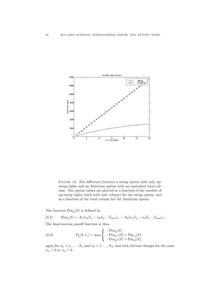
![22 ALI LARI-LAVASSANI, MOHAMADREZA SIMCHI, AND ANTONY WARE
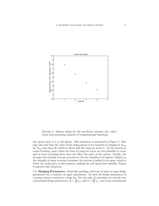
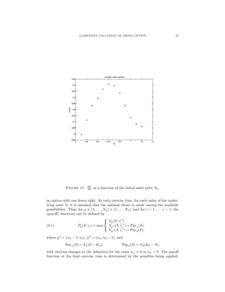
Figure 10. Λ as a function of the initial asset price S0.
We limit the exposition to the proof of convergence for the one-factor mean-
reverting binomial model described in Theorem 1, and note that the result could
be readily adapted to cover other one-factor trees. The proof for the two-factor
case would be similar in structure but rather more involved.
8.1. The Swing Option as a Coupled System of European Options. Con-
sider the option described in Section 5, and write ν = (nu, nd). Let Vν(S, t) be
the value at time t ∈ [0, T2] of an option with nu up-swing rights and nd down-
swing rights remaining, given an asset price of S at time t. Noting that the holder
of such an option may choose to exercise at the exercise times t ∈ {τ1, . . . , τe},
we see that Vν(S, t) may have a jump discontinuity at those times. We write
Vν(S, τ+
i ) = limt→τ+
i
Vν(S, t).
As described in Section 6, the exercise of a swing right brings with it an associ-
ated cash flow, but also means that the option value is exchanged for the value of](https://image.slidesharecdn.com/2e137caa-c106-45e4-b98c-2c28cf277cf9-170125135748/85/SwingOptions-22-320.jpg)
![A DISCRETE VALUATION OF SWING OPTION 25
For t in the interval (τi, τi+1), the option value Vk,l(S, t) is the value of a Euro-
pean contract at time t with expiry at time τi+1 and payoff function Pν(S, τi+1).
The value of this swing option in any given time interval thus depends (via the
payoff function) on the values of related swing options in subsequent time intervals.
In particular, the value of the original swing contract is Vν0 (S0, 0). This is the
value at time 0 and asset price S0 of a European option with expiry time τ1 and
payoff Pν0 (S, τ1), and thus depends on the values of all of the swing options in the
subsequent time intervals.
Obtaining a value for Vν0 (S0, 0) thus involves, for i running backwards from e−1
to 1, first calculating each Pν(S, τi+1) via (8.1) or (8.3), and then evaluating the
European options described above in the interval (τi, τi+1). These values are then
used to calculate the next set of payoff functions. Finally, the European option
with expiry time τ1 and payoff Pν0 (S, τ1) is used to provide the required value at
S = S0 and t = 0.
8.2. A Partial Differential Equation Model. The question remains of how
the European options described above are to be valued. Here we describe a partial
differential equation model based on a generalization of the Black-Scholes equation,
Vt +
σ2
2
S2
VSS + rSVS = rV.
This models, for example, the price V of a stock with volatility σ and risk-free
interest rate r contingent on a stock price S which follows the stochastic process
(2.2). The complete-market assumptions which underlies this model may not apply
in the context we are interested in. Relaxing these assumptions somewhat, we have
the equation
Vt +
σ2
2
S2
VSS + (µ − λσS)VS = rV,
where S is now assumed to follow the stochastic process (2.3), and λ is the market
price of risk function (See [H, 1999], [W, 1998]). We assume for ease of exposition
that λ = 0. The results obtained in this section would hold equally well for other
forms of λ satisfying quite mild continuity assumptions.
We make two concessions to our numerical schemes in the model we describe.
The first is that we impose a lower bound Smin > 0 on the asset price S. The
second is due to the fact that the payoff functions described above are continuous,
but are only piecewise differentiable. This lack of smoothness introduces theoretical
problems for the convergence of numerical schemes such as those described here.
We define a ‘mollified’ maximum function, max , by means of a formula such as
max (a, b) =
a + b + + (a − b)2)
2
,
with
max (a, b, c) = max (a, max (b, c)).
Note that when = 0 this definition agrees with the standard definition of the
maximum. However, defining the payoff functions using max instead of max means
that the payoff functions Pν(S, τi) in (8.1) are just as smooth as the functions
Vν(S, τ+
i ) used to define them. As long as is chosen sensibly, it is easy to verify
that the effect on the option price is negligible.](https://image.slidesharecdn.com/2e137caa-c106-45e4-b98c-2c28cf277cf9-170125135748/85/SwingOptions-25-320.jpg)
![26 ALI LARI-LAVASSANI, MOHAMADREZA SIMCHI, AND ANTONY WARE
We are now ready to describe our partial differential equation model for the value
of a swing option.
Let Smin > 0, σ > 0 and r ≥ 0 be constants. We seek a set of functions Vν(S, t)
satisfying
∂
∂t
Vν(S, t) +
σ2
S2
2
∂2
∂S2
Vν(S, t) + (AS + B)
∂
∂S
Vν(S, t) = rSVν(S, t),
for S > Smin, t ∈ [0, T]{τi}e
i=1, with
Vν(S, T) = max (−Penν(S), −Penνu (S) + Payu(S),(8.4)
− Penνd (S) + Payd(S)),
Vν(S, τi) = max (Vν(S, τ+
i ), Vνu (S, τ+
i ) + Payu(S),(8.5)
Vνd (S, τ+
i ) + Payd(S)), i = 1, . . . , e − 1
∂
∂S
Vν(Smin, t) = 0, t ∈ [0, T].(8.6)
The comparison with the binomial scheme will in fact be more straightforward if
we describe the equivalent log-transformed problem for wν(x, t) = e−r(T −t)
Vν(S, t):
∂
∂t
wν(x, t) +
σ2
2
∂2
∂x2
wν(x, t) + (a + be−x
)
∂
∂x
wν(x, t) = 0,(8.7)
for x > ln Smin, t ∈ [0, T]{τi}e
i=1, with
wν(x, T) = max (−Penν(ex
), −Penνu (ex
) + Payu(ex
),(8.8)
− Penνd (ex
) + Payd(ex
)),
wν(x, τi) = max (wν(x, τ+
i ), wνu (x, τ+
i ) + Payu(ex
),(8.9)
wνd (x, τ+
i ) + Payd(ex
)), i = 1, . . . , e − 1
∂
∂x
wν(ln Smin, t) = 0, t ∈ [0, T],(8.10)
where a = A − σ2
/2 and b = B.
8.3. The One-factor Binomial Scheme. The binomial approximation to the
above partial differential equation model consists in finding vectors Wi
ν(j) satisfy-
ing, for j ≥ jmin,
Wi,∗
ν (j) = pjWi+1
ν (j + 1) + (1 − pj)Wi+1
ν (j − 1), i < T/∆t = N2n,
WN2n,∗
ν (j) = −Penν(exj
),
Wi
ν(j) = Wi,∗
ν (j), i + 1 ∈ Ie
Wi
ν(j) = max Wi,∗
ν (j), Wi,∗
νu (j) + Payu(exj
), Wi,∗
νd (j) + Payd(exj
) , i + 1 ∈ Ie.
Here xj = ln(S0ej∆x
), with ∆x = σ
√
∆t, and jmin is the value of j for which
Sj = exj
= Smin. The above system is completed by setting
Wi+1
ν (jmin − 1) = Wi+1
ν (jmin + 1),
thus approximating the zero-derivative boundary condition at Smin. The required
option value is obtained once W0
ν0 (0) is obtained. Note that not all values of Wi
ν(j)
are required in order to achieve this. For instance, Wi
ν(j) with i+j odd never needs
to be calculated. Moreover, only values with |j| ≤ i can ever affect W0
ν0 (0).](https://image.slidesharecdn.com/2e137caa-c106-45e4-b98c-2c28cf277cf9-170125135748/85/SwingOptions-26-320.jpg)
![A DISCRETE VALUATION OF SWING OPTION 27
8.4. Convergence of the Value of the Swing Option. Here we write wi
ν(j) =
wν(Sj, t+
i ), with ti = i∆t, and denote the difference between the result of the
binomial calculation and the true solution of the partial differential equation model
by ei
ν(j) = Wi
ν(j) − wi
ν(j). Then we have the following global convergence result
for the binomial forest method.
Theorem 3 (Convergence). Suppose that for each x ∈ [xmin, ∞), wν(x, t) is con-
tinuous on (τi, τi+1] for i = 1, . . . , e and on [0, τ1], and that ∂2
∂t2 wν(x, t) exists and
is bounded on each of these intervals. Suppose also that for each t ∈ [0, T2], wν(x, t)
is three times continuously differentiable, with bounded derivatives up to order four
on (xmin, ∞). Then there exists a constant C such that for each ν,
max
i
max
j
ei
ν(j) ≤ C∆t.
The remainder of this section will be taken up with the proof of Theorem 3.
Substituting the vectors ei
ν(j) into the binomial scheme yields, for j > jmin,
ei,∗
ν (j) = pjei+1
ν (j + 1) + (1 − pj)ei+1
ν (j − 1) + Ti
ν(j), i < N2n(8.11)
ei,∗
ν (j) = 0, i = N2n
ei
ν(j) = ei,∗
ν (j), i + 1 ∈ Ie,(8.12)
ei
ν(j) = max Wi,∗
ν (j), Wi,∗
νu (j) + Payu(exj
), Wi,∗
νd (j) + Payd(exj
) −(8.13)
max wi,∗
ν (j) + Ti
ν(j), wi,∗
νu (j) + Ti
νu (j) + Payu(exj
),
wi,∗
νd (j) + Ti
νd (j) + Payd(exj
) i + 1 ∈ Ie,
where the truncation error Ti
ν(j), which will be the amount by which wi
ν(j) fails
to satisfy the equations defining the binomial approximation, is given by
Ti
ν(j) = wi,∗
ν (j) − wi
ν(j),(8.14)
and
wi,∗
ν (j) = pjwi+1
ν (j + 1) + (1 − pj)wi+1
ν (j − 1) = Wi,∗
ν (j) − ei,∗
ν (j)
for j > jmin. To completely specify the error, we need the boundary equation
ei
ν(jmin) = ei+1
ν (jmin + 1) + Ti
ν(jmin),(8.15)
where
Ti
ν(jmin) = wi+1
ν (jmin + 1) − wi
ν(jmin).(8.16)
We shall restrict our attention to relevant values of j: for each i we only consider
j ∈ Ji with
Ji = {j : j + i even, j ≥ jmin, |j| ≤ i}.
It will be shown inductively that the maximum error ei
= maxν,j∈Ji
ei
ν(j) is
O(∆t). In order to do this, is it necessary to get a handle on the truncation error
terms.](https://image.slidesharecdn.com/2e137caa-c106-45e4-b98c-2c28cf277cf9-170125135748/85/SwingOptions-27-320.jpg)
![A DISCRETE VALUATION OF SWING OPTION 29
for all a, b, c, a , b , c ∈ R. Then it follows from (8.13) that, when i + 1 ∈ Ie and
j > jmin,
ei
ν(j) ≤ C3 max ei+1
ν (j) + Ti
ν(j) , ei+1
νu (j) + Ti
νu (j) , ei+1
νd (j) + Ti
νd (j) ,
with obvious changes for the cases nu = 0 and nd = 0, so that
ei
≤ C3 max ei+1
+ C2∆t2
, C1∆t) .(8.20)
Comparing (8.19) and (8.20), we find that they differ only by the extra factor of
C3 when i+1 ∈ Ie. For each i, define k(i) to be the size of the set {i ≥ k : i+1 ∈ Ie}.
Then we make the inductive claim
ei
≤ C
k(i)
3 C1∆t + C2∆t2
(nN2 − i) .
Since eN2n
= 0, the inductive hypothesis holds for i = N2n. Suppose that it holds
for i = i + 1. Then if i + 1 ∈ Ie,
ei
≤ C3 max ei +1
+ C2∆t2
, C1∆t)
≤ C3C
k(i +1)
3 C1∆t + C2∆t2
(nN2 − i − 1) + C2∆t2
= C
k(i )
3 C1∆t + C2∆t2
(nN2 − i )
so that the inductive step is complete in this case. The proof in the case i + 1 ∈ Ie
is exactly similar, and so the theorem is proved, with
C = C
k(0)
3 (C1 + C2T2).
REFERENCES
[BG, 1996] Berbieri, Angelo and Garman, Mark B. October 1996. Putting a Price on
Swings. Energy & Power Risk Management.
[G, 1997] Gardiner, Crispin W. 1997. Handbook of Stochastic Methods. Springer.
[JRT, 1998] Jaillet Patrick, Ronn Ehud I. and Tompaidis Stathis. 1998. Modeling Energy
Prices and Pricing and Hedging Energy Derivatives. Preprint.
[H, 1999] Hull, John. 1999. Options, Futures and Other Derivative Securities. Prentice
Hall.
[HR, 1998] Hilliard Jimmy E and Reis Jorge. 1998. Valuation of Commodity Futures
and Options under Stochastic Convenience Yields, Interest Rates, and Jump
Diffusions in the Spot. J. of Financial and Quantitative Analysis, Vol. 33,
No. 1, pp. 61-86.
[HS, 1974] Hirsch Morris and Smale Stephen. 1974. Differential Equations, Dynamical
Systems and Linear Algebra. Academic Press.
[KP, 1999] Kloeden Peter E. and Platen Eckhard. 1995. Numerical Solution of Stochas-
tic Differential Equations. Springer-Verlag.](https://image.slidesharecdn.com/2e137caa-c106-45e4-b98c-2c28cf277cf9-170125135748/85/SwingOptions-29-320.jpg)
![30 ALI LARI-LAVASSANI, MOHAMADREZA SIMCHI, AND ANTONY WARE
[K, 1998] Kwok Yue-Kuen. 1998. Mathematical Models of Financial Derivatives. Springer-
Verlag.
[P, 1997] Pilipovic Dragana. 1997. Valuing and Managing Energy Derivatives. McGraw-
Hill.
[R, 1995] Robinson Clark. 1995. Dynamical Systems. CRC Press.
[S, 1998] Schwartz Eduardo S. 1998.Valuing Long-Term Commodity Assets. Financial
Management, Vol. 27, No. 1, pp. 57-66.
[W, 1998] Wilmott, Paul. 1998. Derivatives: The Theory and Practice of Financial
Engineering. John Wiley & Sons.
The Mathematical and Computational Finance Laboratory. Department of Mathe-
matics and Statistics. University of Calgary. Calgary, Alberta N1G 4Z4 Canada
E-mail address: lavassan@math.ucalgary.ca
simchi@math.ucalgary.ca
ware@math.ucalgary.ca](https://image.slidesharecdn.com/2e137caa-c106-45e4-b98c-2c28cf277cf9-170125135748/85/SwingOptions-30-320.jpg)