
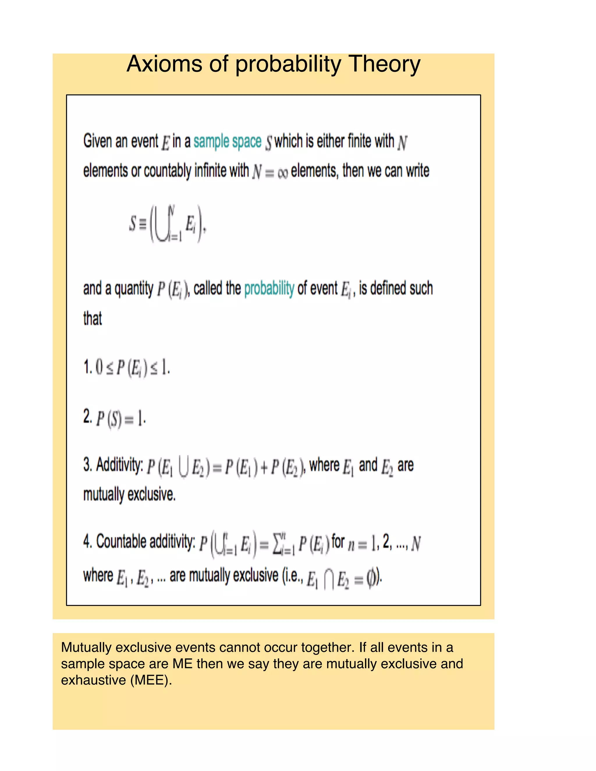
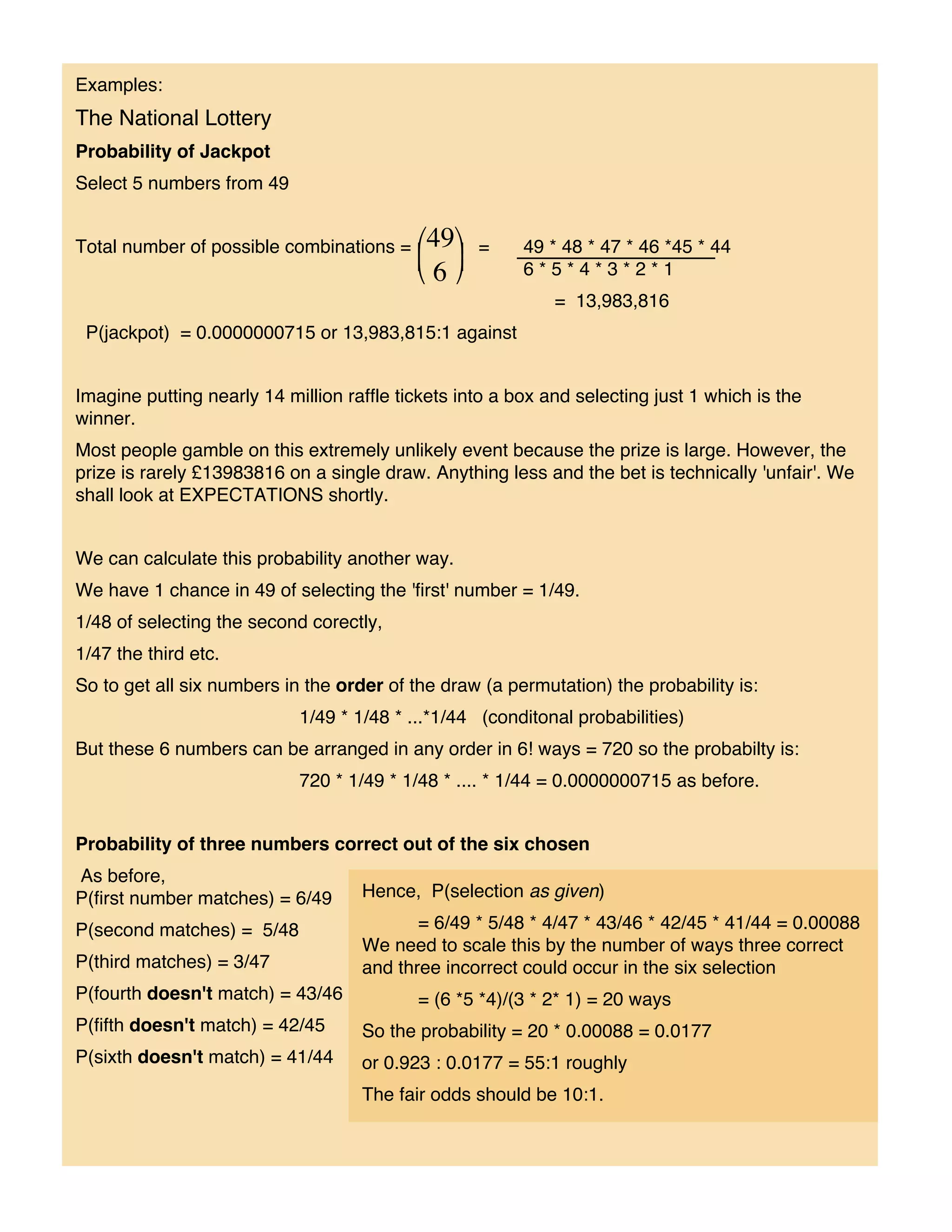
![NOTE: The probabilty that E does NOT occur is:
If P(E) = 1 => E certain to occur
If P(E) = 0 => E certain not to occur
Outcome spaces (sets)
This is a description of the outcomes of interest in the calculation of
probabilities.
For gambling situation this could be simply:
S = { win, lose} and P(win) = 0.4 and P(lose) = 0.6
The events 'win' and 'lose' would be associated with the outcome of the gamble
(or trial).
Thus, if we were to toss two (fair) coins and gamble on the occurrence of two
heads occuring, then:
S = {[H,H], [H,T], [T,H], [T,T]} assuming equally likely outcomes.
P(win) = p([H,H]) = 1/4 and P(lose) = 3/4
If we bet on the faces being different i.e. the COMBINATION {H,T} occurs
then P({H,T})
=
or put simply 2 cases out of four
[ Note:In this trial we could toss a single coin twice instead of tossing two coins
and we assume P(coin lands on edge) = 0]](https://image.slidesharecdn.com/brianprior-probabilityandgambling-110603074332-phpapp02/75/Brian-Prior-Probability-and-gambling-6-2048.jpg)
![Poker
The probabilities of getting the various hands at poker (e.g. four of a kind, pair,
two pair etc) can be found using the theoretical results we have already looked
at. However, calculating these probabilites can be quite tricky!
Hand Probability Distribution
No pair 1,303,560 in 2,598,960 50 .16%
One pair 1,098,240 in 2,598,960 42 .26%
Two pair 123,552 in 2,598,960 4 .75%
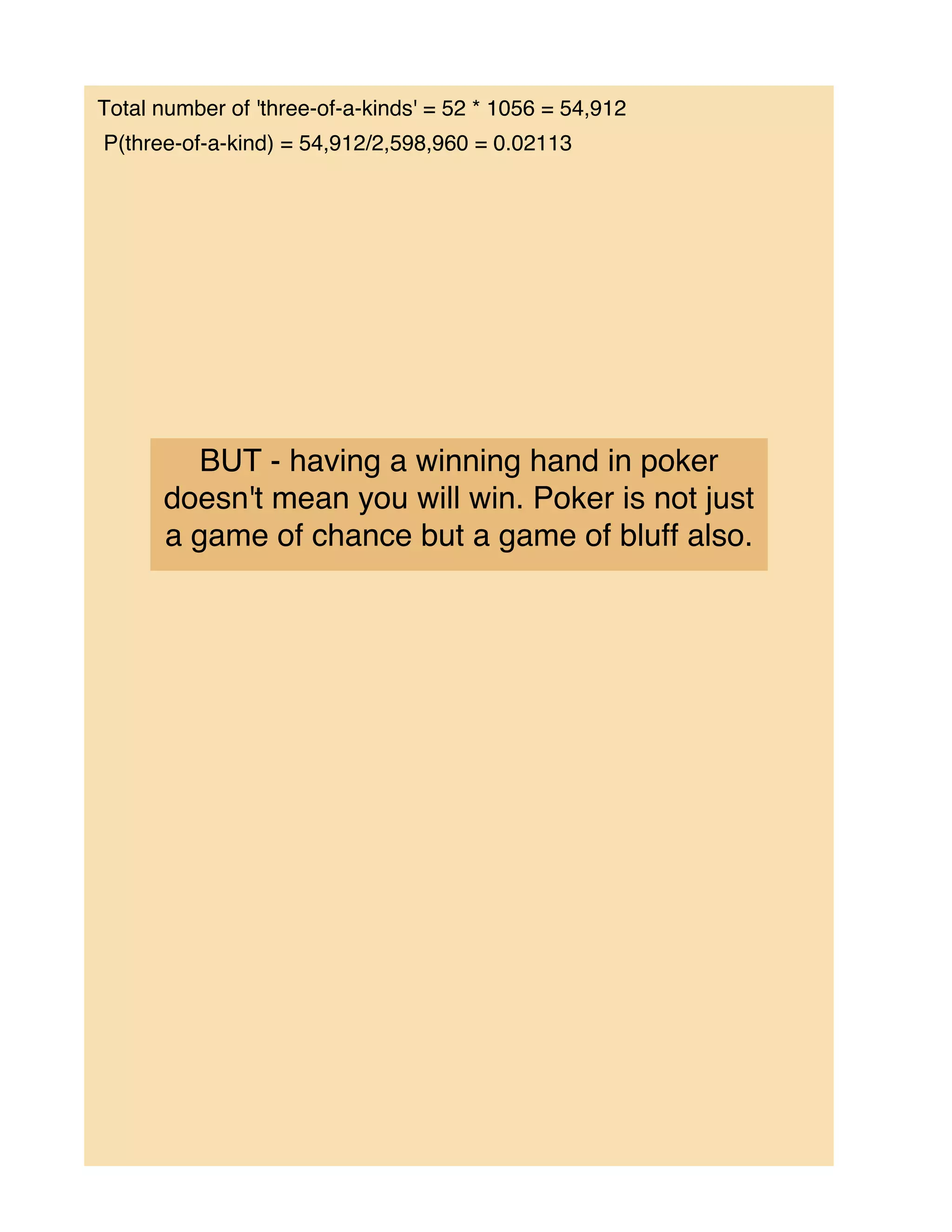
Three of a kind 54,912 in 2,598,960 2 .11%
Straight 9,180 in 2,598,960 0 .353%
Flush 5,112 in 2,598,960 0 .197%
Full house 3,744 in 2,598,960 0 .144%
Four of a kind 624 in 2,598,960 0 .0240%
Straight flush (excluding Royal flush) 32 in 2,598,960 0 .00123%
Royal straight flush 4 in 2,598,960 0 .000154%
TOTAL 2,598,960 in 2,598,960 100
The total number of five card hands = 52C5 = 2,598,960 different hands
Example calculation:
Probability of three of a kind (e.g. three kings and any two others [not pairs])
For convenience let
For a given rank of four cards (e.g. Kh,Kd,Ks,Kc) we can select any three in 4C3
= 4 ways.
We have 13 ranks so we can create 13 * 4 = 52 different triples ('three-of-a-
kinds'.)
Now consider those cards not in the rank of the triple. We have 12 ranks in the
four suits and and we can select any pair that are not the same rank. We have
12 ranks to choose from. Ignoring suits for the present we can select 12C2 pairs
among any rank (so no pairs) and each number in the pair could come from four
suits, so the total number of different pairs is 12C2 x 42 = 1056](https://image.slidesharecdn.com/brianprior-probabilityandgambling-110603074332-phpapp02/75/Brian-Prior-Probability-and-gambling-16-2048.jpg)

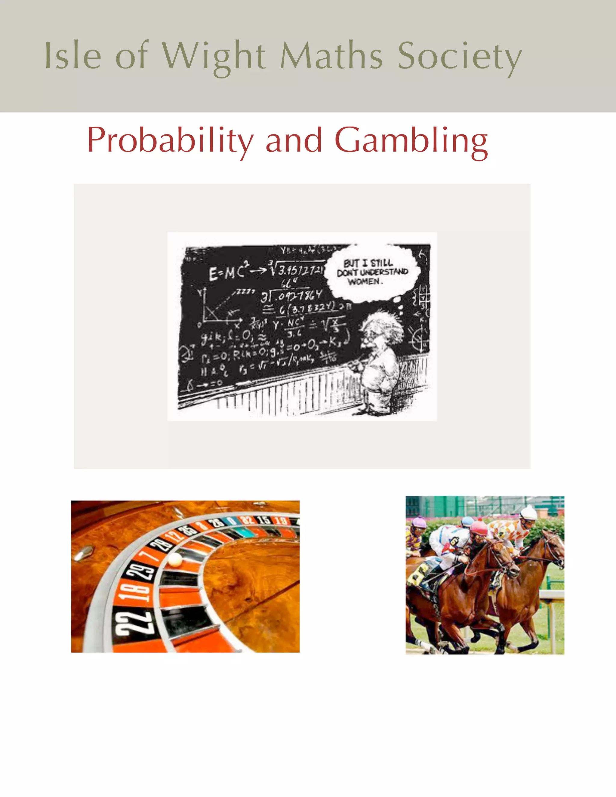
This document discusses probability theory and its applications to gambling. It begins with a brief history of probability theory and its development from Pascal and Fermat's work on gambling disputes. It then covers key concepts like defining probability, outcome spaces, the axioms of probability, and examples of counting combinations and permutations. The document also discusses important probability distributions like the binomial distribution and conditional probability. It provides gambling examples to illustrate concepts like expected value, fairness of bets, and how casinos ensure a house edge through payout odds.


![Probability[1]](https://cdn.slidesharecdn.com/ss_thumbnails/probability1-110816105858-phpapp02-thumbnail.jpg?width=640&height=640&fit=bounds)


