
More Related Content
Similar to chap2p.pdf
Similar to chap2p.pdf (20)
Recently uploaded
Recently uploaded (20)
chap2p.pdf
- 1. Chapter 2 Probability From Probability, For the Enthusiastic Beginner (Draft version, March 2016) David Morin, morin@physics.harvard.edu Having learned in Chapter 1 how to count things, we can now talk about probability. We will find that in many situations it is a trivial matter to generate probabilities from our counting results. So we will be justly rewarded for the time and effort we spent in Chapter 1. The outline of this chapter is as follows. In Section 2.1 we give the definition of probability. Although this definition is fairly easy to apply in most cases, there are a number of subtleties that come up. These are discussed in Appendix A. In Section 2.2 we present the various rules of probability. We show how these can be applied in a few simple examples, and then we work through a number of more substantial examples in Section 2.3. In Section 2.4 we present four classic prob- ability problems that many people find counterintuitive. Section 2.5 is devoted to Bayes’ theorem, which is a relation between certain conditional probabilities. Fi- nally, in Section 2.6 we discuss Stirling’s formula, which gives an approximation to the ubiquitous factorial, n!. 2.1 Definition of probability Probability gives a measure of how likely it is for something to happen. It can be defined as follows: Definition of probability: Consider a very large number of identical trials of a certain process; for example, flipping a coin, rolling a die, picking a ball from a box (with replacement), etc. If the probability of a particular event occurring (for example, getting a Heads, rolling a 5, or picking a blue ball) is p, then the event will occur in a fraction p of the trials, on average. Some examples are: • The probability of getting a Heads on a coin flip is 1/2 (or equivalently 50%). This is true because the probabilities of getting a Heads or a Tails are equal, which means that these two outcomes must each occur half of the time, on average. 57
- 2. 58 Chapter 2. Probability • The probability of rolling a 5 on a standard 6-sided die is 1/6. This is true because the probabilities of rolling a 1, 2, 3, 4, 5, or 6 are all equal, which means that these six outcomes must each happen one sixth of the time, on average. • If there are three red balls and seven blue balls in a box, then the probabilities of picking a red ball or a blue ball are, respectively, 3/10 and 7/10. This follows from the fact that the probabilities of picking each of the ten balls are all equal (or at least let’s assume they are), which means that each ball will be picked one tenth of the time, on average. Since there are three red balls, a red ball will therefore be picked 3/10 of the time, on average. And since there are seven blue balls, a blue ball will be picked 7/10 of the time, on average. Note the inclusion of the words “on average” in the above definition and examples. We’ll discuss this in detail in the subsection below. Many probabilistic situations have the property that they involve a number of different possible outcomes, all of which are equally likely. For example, Heads and Tails on a coin are equally likely to be tossed, the numbers 1 through 6 on a die are equally likely to be rolled, and the ten balls in the above box are all equally likely to be picked. In such a situation, the probability of a certain scenario happening is given by p = number of desired outcomes total number of possible outcomes (for equally likely outcomes) (2.1) Calculating a probability then simply reduces to a matter of counting the number of desired outcomes, along with the total number of outcomes. For example, the probability of rolling an even number on a die is 1/2, because there are three desired outcomes (2, 4, and 6) and six total possible outcomes (the six numbers). And the probability of picking a red ball in the above example is 3/10, as we already noted, because there are three desired outcomes (picking any of the three red balls) and ten total possible outcomes (the ten balls). These two examples involved trivial counting, but we’ll encounter many examples where it is more involved. This is why we did all of that counting in Chapter 1! It should be stressed that Eq. (2.1) holds only under the assumption that all of the possible outcomes are equally likely. But this usually isn’t much of a restriction, because this assumption will generally be valid in the setups we’ll be dealing with in this book. In particular, it holds in setups dealing with permutations and subgroups, both of which we studied in detail in Chapter 1. Our ability to count these sorts of things will allow us to easily calculate probabilities via Eq. (2.1). Many examples are given in Section 2.3 below. There are three words that people often use interchangeably: “probability,” “chance,” and “odds.” The first two of these mean the same thing. That is, the statement, “There is a 40% chance that the bus will be late,” is equivalent to the statement, “There is a 40% probability that the bus will be late.” However, the word “odds” has a different meaning; see Problem 2.1 for a discussion of this.
- 3. 2.2. The rules of probability 59 The importance of the words “on average” The above definition of probability includes the words “on average.” These words are critical, because the definition wouldn’t make any sense if we omitted them and instead went with something like: “If the probability of a particular event occurring is p, then the event will occur in exactly a fraction p of the trials.” This can’t be a valid definition of probability, for the following reason. Consider the roll of one die, for which the probability of each number occurring is 1/6. This definition would imply that on one roll of a die, we will get 1/6 of a 1, and 1/6 of a 2, and so on. But this is nonsense; you can’t roll 1/6 of a 1. The number of times a 1 appears on one roll must of course be either zero or one. And in general for many rolls, the number must be an integer, 0, 1, 2, 3, .... There is a second problem with this definition, in addition to the problem of non integers. What if we roll a die six times? This definition would imply that we will get exactly (1/6) · 6 = 1 of each number. This prediction is a little better, in that at least the proposed numbers are integers. But it still can’t be correct, because if you actually do the experiment and roll a die six times, you will find that you are certainly not guaranteed to get each of the six numbers exactly once. This scenario might happen (we’ll calculate the probability in Section 2.3.4 below), but it is more likely that some numbers will appear more than once, while other numbers won’t appear at all. Basically, for a small number of trials (such as six), the fractions of the time that the various events occur will most likely not look much like the various probabili- ties. This is where the words “very large number” in our original definition come in. The point is that if you roll a die a huge number of times, then the fractions of the time that each of the six numbers appears will be approximately equal to 1/6. And the larger the number of rolls, the closer the fractions will generally be to 1/6. In Chapter 5 we’ll explain why the fractions are expected to get closer and closer to the actual probabilities, as the number of trials gets larger and larger. For now, just take it on faith that if you flip a coin 100 times, the probability of obtaining either 49, 50, or 51 Heads isn’t so large. It happens to be about 24%, which tells you that there is a decent chance that the fraction of Heads will deviate moderately from 1/2. However, if you flip a coin 100,000 times, the probability of obtaining Heads between 49% and 51% of the time is 99.999999975%, which tells you that there is virtually no chance that the fraction of Heads will deviate much from 1/2. If you increase the number of flips to 109 (a billion), this result is even more pronounced; the probability of obtaining Heads in the narrow range between 49.99% and 50.01% of the time is 99.999999975% (the same percentage as above). We’ll discuss such matters in detail in Section 5.2. For more commentary on the words “on average,” see the last section in Appendix A. 2.2 The rules of probability So far we’ve talked only about the probabilities of single events, for example, rolling an even number on a die, getting a Heads on a coin toss, or picking a blue ball from a box. We’ll now consider two (or more) events. Reasonable questions we
- 4. 60 Chapter 2. Probability can ask are: What is the probability that both of the events occur? What is the probability that either of the events occurs? The rules presented below will answer these questions. We’ll provide a few simple examples for each rule, and then we’ll work through some longer examples in Section 2.3. 2.2.1 AND: The “intersection” probability, P(A and B) Let A and B be two events. For example, if we roll two dice, we can let A = {rolling a 2 on the left die} and B = {rolling a 5 on the right die}. Or we might have A = {picking a red ball from a box} and B = {picking a blue ball without replacement after the first pick}. What is the probability that A and B both occur? In answering this question, we must consider two cases: (1) A and B are independent events, or (2) A and B are dependent events. Let’s look at each of these in turn. In each case, the probability that A and B both occur is known as the joint probability. Independent events Two events are said to be independent if they don’t affect each other, or more pre- cisely, if the occurrence of one doesn’t affect the probability that the other occurs. An example is the first setup mentioned above – rolling two dice, with A = {rolling a 2 on the left die} and B = {rolling a 5 on the right die}. The probability of ob- taining a 5 on the right die is 1/6, independent of what happens with the left die. And similarly the probability of obtaining a 2 on the left die is 1/6, independent of what happens with the right die. Independence requires that neither event affects the other. The events in the second setup mentioned above with the balls in the box are not independent; we’ll talk about this below. Another example of independent events is picking one card from a deck, with A = {the card is a king} and B = {the (same) card is a heart}. The probability of the card being a heart is 1/4, independent of whether or not it is a king. And the probability of the card being a king is 1/13, independent of whether or not it is a heart. Note that it is possible to have two different events even if we have only one card. This card has two qualities (its suit and its value), and we can associate an event with each of these qualities. Remark: A note on terminology: The words “event” and “outcome” sometimes mean the same thing in practice, but there is technically a difference. An outcome is the result of an experiment. If we draw a card from a deck, then there are 52 possible outcomes; for example, the 4 of clubs, the jack of diamonds, etc. An event is a set of outcomes. For example, an event might be “drawing a heart.” This event contains 13 outcomes, namely the 13 cards that are hearts. A given card may belong to many events. For example, in addition to belonging to the A and B events in the preceding paragraph, the king of hearts belongs to the events C = {the card is red}, D = {the card’s value is higher than 8}, E = {the card is the king of hearts}, and so on. As indicated by the event E, an event may consist of a single outcome. An event may also be the empty set (which occurs with probability 0), or the entire set of all possible outcomes (which occurs with probability 1), which is known as the sample space. ♣
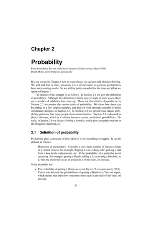
- 5. 2.2. The rules of probability 61 The “And” rule for independent events is: • If events A and B are independent, then the probability that they both occur equals the product of their individual probabilities: P(A and B) = P(A) · P(B) (2.2) We can quickly apply this rule to the two examples mentioned above. The prob- ability of rolling a 2 on the left die and a 5 on the right die is P(2 and 5) = P(2) · P(5) = 1 6 · 1 6 = 1 36 . (2.3) This agrees with the fact that one out of the 36 pairs of (ordered) numbers in Table 1.5 is “2, 5.” Similarly, the probability that a card is both a king and a heart is P(king and heart) = P(king) · P(heart) = 1 13 · 1 4 = 1 52 . (2.4) This makes sense, because one of the 52 cards in a deck is the king of hearts. The logic behind Eq. (2.2) is the following. Consider N trials of a given process, where N is very large. In the case of the two dice, a trial consists of rolling both dice. The outcome of such a trial takes the form of an ordered pair of numbers. The first number is the result of the left roll, and the second number is the result of the right roll. On average, the fraction of the outcomes that have a 2 as the first number is (1/6) · N. Let’s now consider only this “2-first” group of outcomes and ignore the rest. Then on average, a fraction 1/6 of these outcomes have a 5 as the second number. This is where we are invoking the independence of the events. As far as the second roll is concerned, the set of (1/6)· N trials that have a 2 as the first roll is no different from any other set of (1/6)·N trials, so the probability of obtaining a 5 on the second roll is simply 1/6. Putting it all together, the average number of trials that have both a 2 as the first number and a 5 as the second number is 1/6 of (1/6) · N, which equals (1/6) · (1/6) · N. In the case of general probabilities P(A) and P(B), it is easy to see that the two (1/6)’s in the above result get replaced by P(A) and P(B). So the average number of outcomes where A and B both occur is P(A)·P(B)·N. And since we performed N trials, the fraction of outcomes where A and B both occur is P(A)·P(B), on average. From the definition of probability in Section 2.1, this fraction is the probability that A and B both occur, in agreement with Eq. (2.2). If you want to think about the rule in Eq. (2.2) in terms of a picture, then consider Fig. 2.1. Without worrying about specifics, let’s assume that different points within the overall square represent different outcomes. And let’s assume that they’re all equally likely, which means that the area of a region gives the probability that an outcome located in that region occurs (assuming that the area of the whole region is 1). The figure corresponds to P(A) = 0.2 and P(B) = 0.4. Outcomes to the left of the vertical line are ones where A occurs, and outcomes to the right of the vertical line are ones where A doesn’t occur. Likewise for B and outcomes above and below the horizontal line.
- 6. 62 Chapter 2. Probability A B not A 20% of the width 40% of the height not B A and B B and not A A and not B not A and not B Figure 2.1: A probability square for independent events. From the figure, we see that not only is 40% of the entire square above the vertical line, but also that 40% of the left vertical strip (where A occurs) is above the vertical line, and likewise for the right vertical strip (where A doesn’t occur). In other words, B occurs 40% of the time, independent of whether or not A occurs. Basically, B couldn’t care less what happens with A. Similar statements hold with A and B interchanged. So this type of figure, with a square divided by horizontal and vertical lines, does indeed represent independent events. The darkly shaded “A and B” region is the intersection of the region to the left of the vertical line (where A occurs) and the region above the horizontal line (where B occurs). Hence the word “intersection” in the title of this section. The area of the darkly shaded region is 20% of 40% (or 40% of 20%) of the total area, that is, (0.2)(0.4) = 0.08 of the total area. The total area corresponds to a probability of 1, so the darkly shaded region corresponds to a probability of 0.08. Since we obtained this probability by multiplying P(A) by P(B), we have therefore given a pictorial proof of Eq. (2.2). Dependent events Two events are said to be dependent if they do affect each other, or more precisely, if the occurrence of one does affect the probability that the other occurs. An example is picking two balls in succession from a box containing two red balls and three blue balls (see Fig. 2.2), with A = {choosing a red ball on the first pick} and B = {choosing a blue ball on the second pick, without replacement after the first pick}. If you pick a red ball first, then the probability of picking a blue ball second is 3/4, because there are three blue balls and one red ball left. On the other hand, if you don’t pick a red ball first (that is, if you pick a blue ball first), then the probability of picking a blue ball second is 2/4, because there are two red balls and two blue balls left. So the occurrence of A certainly affects the probability of B. Another example might be something like: A = {it rains at 6:00} and B = {you walk to the store at 6:00}. People are generally less likely to go for a walk when it’s raining outside, so (at least for most people) the occurrence of A affects the probability of B.
- 7. 2.2. The rules of probability 63 Red Red Blue Blue Blue Figure 2.2: A box with two red balls and three blue balls. The “And” rule for dependent events is: • If events A and B are dependent, then the probability that they both occur equals P(A and B) = P(A) · P(B|A) (2.5) where P(B|A) stands for the probability that B occurs, given that A occurs. It is called a “conditional probability,” because we are assuming a given condition, namely that A occurs. It is read as “the probability of B, given A.” There is actually no need for the “dependent” qualifier in the first line of this rule, as we’ll see in the second remark near the end of this section. The logic behind Eq. (2.5) is the following. Consider N trials of a given process, where N is very large. In the above setup with the balls in a box, a “trial” consists of picking two balls in succession, without replacement. On average, the fraction of the outcomes in which a red ball is drawn on the first pick is P(A) · N. Let’s now consider only these outcomes and ignore the rest. Then a fraction P(B|A) of these outcomes have a blue ball drawn second, by the definition of P(B|A). So the number of outcomes where A and B both occur is P(B|A) · P(A) · N. And since we performed N trials, the fraction of outcomes where A and B both occur is P(A) · P(B|A), on average. This fraction is the probability that A and B both occur, in agreement with the rule in Eq. (2.5). The reasoning in the previous paragraph is equivalent to the mathematical iden- tity, nA and B N = nA N · nA and B nA , (2.6) where nA is the number of trials where A occurs, etc. By definition, the lefthand side of this equation equals P(A and B), the first term on the righthand side equals P(A), and the second term on the righthand side equals P(B|A). So Eq. (2.6) is equivalent to the relation, P(A and B) = P(A) · P(B|A), (2.7) which is Eq. (2.5). In terms of the Venn-diagram type of picture in Fig. 2.3, Eq. (2.6) is the statement that the darkly shaded area (which represents P(A and B)) equals the area of the A region (which represents P(A)) multiplied by the fraction of the A region that is taken up by the darkly shaded region. This fraction is P(B|A), by definition.
- 8. 64 Chapter 2. Probability A B A and B Figure 2.3: Venn diagram for probabilities of dependent events. As in Fig. 2.1, we’re assuming in Fig. 2.3 that different points within the over- all boundary represent different outcomes, and that they’re all equally likely. This means that the area of a region gives the probability that an outcome located in that region occurs (assuming that the area of the whole region is 1). We’re using Fig. 2.3 for its qualitative features only, so we’re drawing the various regions as general blobs, as opposed to the specific rectangles in Fig. 2.1, which we used for a quantitative calculation. Because the “A and B” region in Fig. 2.3 is the intersection of the A and B regions, and because the intersection of two sets is usually denoted by A ∩ B, you will often see the P(A and B) probability written as P(A ∩ B). That is, P(A ∩ B) ≡ P(A and B). (2.8) But we’ll stick with the P(A and B) notation in this book. There is nothing special about the order of A and B in Eq. (2.5). We could just as well interchange the letters and write P(B and A) = P(B)·P(A|B). However, we know that P(B and A) = P(A and B), because it doesn’t matter which event you say first when you say that two events both occur. So we can also write P(A and B) = P(B) · P(A|B). Combining this with Eq. (2.5), we see that we can write P(A and B) in two different ways: P(A and B) = P(A) · P(B|A) = P(B) · P(A|B). (2.9) The fact that P(A and B) can be written in these two ways will be critical when we discuss Bayes’ theorem in Section 2.5. Example (Balls in a box): Let’s apply Eq. (2.5) to the setup with the balls in the box in Fig. 2.2 above. Let A = {choosing a red ball on the first pick} and B = {choosing a blue ball on the second pick, without replacement after the first pick}. For shorthand, we’ll denote these events by Red1 and Blue2, where the subscript refers to the first or second pick. We noted above that P(Blue2|Red1) = 3/4. And we also know that P(Red1) is simply 2/5, because there are initially two red balls and three blue balls. So Eq. (2.5) gives the probability of picking a red ball first and a blue ball second (without replacement after the first pick) as P(Red1 and Blue2) = P(Red1) · P(Blue2|Red1) = 2 5 · 3 4 = 3 10 . (2.10)
- 9. 2.2. The rules of probability 65 We can verify that this is correct by listing out all of the possible pairs of balls that can be picked. If we label the balls as 1, 2, 3, 4, 5, and if we let 1, 2 be the red balls, and 3, 4, 5 be the blue balls, then the possible outcomes are shown in Table 2.1. The first number stands for the first ball picked, and the second number stands for the second ball picked. Red first Blue first Red second — 2 1 3 1 4 1 5 1 1 2 — 3 2 4 2 5 2 Blue second 1 3 2 3 — 4 3 5 3 1 4 2 4 3 4 — 5 4 1 5 2 5 3 5 4 5 — Table 2.1: Ways to pick two balls from the box in Fig. 2.2, without replacement. The “—” entries stand for the outcomes that aren’t allowed; we can’t pick two of the same ball, because we’re not replacing the ball after the first pick. The dividing lines are drawn for clarity. The internal vertical line separates the outcomes where a red or blue ball is drawn on the first pick, and the internal horizontal line separates the outcomes where a red or blue ball is drawn on the second pick. The six pairs in the lower left corner are the outcomes where a red ball (numbered 1 and 2) is drawn first and a blue ball (numbered 3, 4, and 5) is drawn second. Since there are 20 possible outcomes in all, the desired probability is 6/20 = 3/10, in agreement with Eq. (2.10). Table 2.1 also gives a verification of the P(Red1) and P(Blue2|Red1) probabilities we wrote down in Eq. (2.10). P(Red1) equals 2/5 because eight of the 20 entries are to the left of the vertical line. And P(Blue2|Red1) equals 3/4 because six of these eight entries are below the horizontal line. The task of Problem 2.4 is to verify that the second expression in Eq. (2.9) also gives the correct result for P(Red1 and Blue2) in this setup. We can think about the rule in Eq. (2.5) in terms of a picture analogous to Fig. 2.1. If we consider the above example with the red and blue balls, then the first thing we need to do is recast Table 2.1 in a form where equal areas yield equal probabilities. If we get rid of the “—” entries in Table 2.1, then all entries have equal probabilities, and we end up with Table 2.2. 1 2 2 1 3 1 4 1 5 1 1 3 2 3 3 2 4 2 5 2 1 4 2 4 3 4 4 3 5 3 1 5 2 5 3 5 4 5 5 4 Table 2.2: Rewriting Table 2.1. In the spirit of Fig. 2.1, this table becomes the square shown in Fig. 2.4. The upper left region corresponds to red balls on both picks. The lower left region
- 10. 66 Chapter 2. Probability corresponds to a red ball and then a blue ball. The upper right region corresponds to a blue ball and then a red ball. And the lower right region corresponds to blue balls on both picks. This figure makes it clear why we formed the product (2/5) · (3/4) in Eq. (2.10). The 2/5 gives the fraction of the outcomes that lie to the left of the vertical line (these are the ones that have a red ball first), and the 3/4 gives the fraction of these outcomes that lie below the horizontal line (these are the ones that have a blue ball second). The product of these fractions gives the overall fraction (namely 3/10) of the outcomes that lie in the lower left region. R1 and R2 R1 and B2 B1 and R2 B1 and B2 B1 R1 B2 R2 R2 B2 40% of the width 25% of the height 50% of the height Figure 2.4: Pictorial representation of Table 2.2. The main difference between Fig. 2.4 and Fig. 2.1 is that the one horizontal line in Fig. 2.1 is now two different horizontal lines in Fig. 2.4. The heights of the horizontal lines in Fig. 2.4 depend on which vertical strip we’re dealing with. This is the visual manifestation of the fact that the red/blue probabilities on the second pick depend on what happens on the first pick. Remarks: 1. The method of explicitly counting the possible outcomes in Table 2.1 shows that you don’t have to use the rule in Eq. (2.5), or similarly the rule in Eq. (2.2), to calculate probabilities. You can often instead just count up the various outcomes and solve the problem from scratch. However, the rules in Eqs. (2.2) and (2.5) allow you to take a shortcut that avoids listing out all the outcomes, which might be rather difficult if you’re dealing with large numbers. 2. The rule in Eq. (2.2) for independent events is a special case of the rule in Eq. (2.5) for dependent events. This is true because if A and B are independent, then P(B|A) is simply equal to P(B), because the probability of B occurring is just P(B), independent of whether or not A occurs. Eq. (2.5) then reduces to Eq. (2.2) when P(B|A) = P(B). Therefore, there was technically no need to introduce Eq. (2.2) first. We could have started with Eq. (2.5), which covers all possible scenarios, and then showed that it reduces to Eq. (2.2) when the events are independent. But pedagogically, it is often better to start with a special case and then work up to the more general case. 3. In the above “balls in a box” example, we encountered the conditional probabil- ity P(Blue2|Red1). We can also talk about the “reversed” conditional probability, P(Red1|Blue2). However, since the second pick happens after the first pick, you might wonder how much sense it makes to talk about the probability of the Red1
- 11. 2.2. The rules of probability 67 event, given the Blue2 event. Does the second pick somehow influence the first pick, even though the second pick hasn’t happened yet? When you make the first pick, are you being affected by a mysterious influence that travels backward in time? No, and no. When we talk about P(Red1|Blue2), or about any other conditional probability in the example, everything we might want to know can be read off from Table 2.1. Once the table has been created, we can forget about the temporal or- der of the events. By looking at the Blue2 pairs (below the horizontal line), we see that P(Red1|Blue2) = 6/12 = 1/2. This should be contrasted with P(Red1|Red2), which is obtained by looking at the Red2 pairs (above the horizontal line); we find that P(Red1|Red2) = 2/8 = 1/4. Therefore, the probability that your first pick is red does depend on whether your second pick is blue or red. But this doesn’t mean that there is a backward influence in time. All it says is that if you perform a large number of trials of the given process (drawing two balls, without replacement), and if you look at all of the cases where your second pick is blue (or conversely, red), then you will find that your first pick is red in 1/2 (or conversely, 1/4) of these cases, on average. In short, the second pick has no causal influence on the first pick, but the after-the-fact knowledge of the second pick affects the probability of what the first pick was. 4. A trivial yet extreme example of dependent events is the two events: A, and “not A.” The occurrence of A highly affects the probability of “not A” occurring. If A occurs, then “not A” occurs with probability zero. And if A doesn’t occur, then “not A” occurs with probability 1. ♣ In the second remark above, we noted that if A and B are independent (that is, if the occurrence of one doesn’t affect the probability that the other occurs), then P(B|A) = P(B). Similarly, we also have P(A|B) = P(A). Let’s prove that one of these relations implies the other. Assume that P(B|A) = P(B). Then if we equate the two righthand sides of Eq. (2.9) and use P(B|A) = P(B) to replace P(B|A) with P(B), we obtain P(A) · P(B|A) = P(B) · P(A|B) =⇒ P(A) · P(B) = P(B) · P(A|B) =⇒ P(A) = P(A|B). (2.11) So P(B|A) = P(B) implies P(A|B) = P(A), as desired. In other words, if B is independent of A, then A is also independent of B. We can therefore talk about two events being independent, without worrying about the direction of the indepen- dence. The condition for independence is therefore either of the relations, P(B|A) = P(B) or P(A|B) = P(A) (independence) (2.12) Alternatively, the condition for independence may be expressed by Eq. (2.2), P(A and B) = P(A) · P(B) (independence) (2.13) because this equation implies (by comparing it with Eq. (2.5), which is valid in any case) that P(B|A) = P(B).
- 12. 68 Chapter 2. Probability 2.2.2 OR: The “union” probability, P(A or B) Let A and B be two events. For example, let A = {rolling a 2 on a die} and B = {rolling a 5 on the same die}. Or we might have A = {rolling an even number (that is, 2, 4, or 6) on a die} and B = {rolling a multiple of 3 (that is, 3 or 6) on the same die}. A third example is A = {rolling a 1 on one die} and B = {rolling a 6 on another die}. What is the probability that either A or B (or both) occurs? In answering this question, we must consider two cases: (1) A and B are exclusive events, or (2) A and B are nonexclusive events. Let’s look at each of these in turn. Exclusive events Two events are said to be exclusive if one precludes the other. That is, they can’t both happen. An example is rolling one die, with A = {rolling a 2 on the die} and B = {rolling a 5 on the same die}. These events are exclusive because it is impossible for one number to be both a 2 and a 5. (The events in the second and third scenarios mentioned above are not exclusive; we’ll talk about this below.) Another example is picking one card from a deck, with A = {the card is a diamond} and B = {the card is a heart}. These events are exclusive because it is impossible for one card to be both a diamond and a heart. The “Or” rule for exclusive events is: • If events A and B are exclusive, then the probability that either of them occurs equals the sum of their individual probabilities: P(A or B) = P(A) + P(B) (2.14) The logic behind this rule boils down to Fig. 2.5. The key feature of this figure is that there is no overlap between the two regions, because we are assuming that A and B are exclusive. If there were a region that was contained in both A and B, then the outcomes in that region would be ones for which A and B both occur, which would violate the assumption that A and B are exclusive. The rule in Eq. (2.14) is simply the statement that the area of the union (hence the word “union” in the title of this section) of regions A and B equals the sum of their areas. There is nothing fancy going on here. This statement is no deeper than the statement that if you have two separate bowls, the total number of apples in the two bowls equals the number of apples in one bowl plus the number of apples in the other bowl. We can quickly apply this rule to the two examples mentioned above. In the example with the die, the probability of rolling a 2 or a 5 on one die is P(2 or 5) = P(2) + P(5) = 1 6 + 1 6 = 1 3 . (2.15) This makes sense, because two of the six numbers on a die are the 2 and the 5. In the card example, the probability of a card being either a diamond or a heart is P(diamond or heart) = P(diamond) + P(heart) = 1 4 + 1 4 = 1 2 . (2.16)
- 13. 2.2. The rules of probability 69 A B Figure 2.5: Venn diagram for the probabilities of exclusive events. This makes sense, because half of the 52 cards in a deck are diamonds or hearts. A special case of Eq. (2.14) is the “Not” rule, which follows from letting B = “not A.” P(A or (not A)) = P(A) + P(not A) =⇒ 1 = P(A) + P(not A) =⇒ P(not A) = 1 − P(A). (2.17) The first equality here follows from Eq. (2.14), because A and “not A” are certainly exclusive events; you can’t both have something and not have it. To obtain the second line in Eq. (2.17), we have used P(A or (not A)) = 1, which holds because every possible outcome belongs to either A or “not A.” Nonexclusive events Two events are said to be nonexclusive if it is possible for both to happen. An example is rolling one die, with A = {rolling an even number (that is, 2, 4, or 6)} and B = {rolling a multiple of 3 (that is, 3 or 6) on the same die}. If you roll a 6, then A and B both occur. Another example is picking one card from a deck, with A = {the card is a king} and B = {the card is a heart}. If you pick the king of hearts, then A and B both occur. The “Or” rule for nonexclusive events is: • If events A and B are nonexclusive, then the probability that either (or both) of them occurs equals P(A or B) = P(A) + P(B) − P(A and B) (2.18) The “or” here is the so-called “inclusive or,” in the sense that we say “A or B occurs” if either or both of the events occur. As with the “dependent” qualifier in the “And” rule in Eq. (2.5), there is actually no need for the “nonexclusive” qualifier in the “Or” rule here, as we’ll see in the third remark below. The logic behind Eq. (2.18) boils down to Fig. 2.6. The rule in Eq. (2.18) is the statement that the area of the union of regions A and B equals the sum of their areas minus the area of the overlap. This subtraction is necessary so that we don’t double
- 14. 70 Chapter 2. Probability count the region that belongs to both A and B. This region isn’t “doubly good” just because it belongs to both A and B. As far as the “A or B” condition goes, the overlap region is just the same as any other part of the union of A and B. A B A and B Figure 2.6: Venn diagram for the probabilities of nonexclusive events. In terms of a physical example, the rule in Eq. (2.18) is equivalent to the state- ment that if you have two bird cages that have a region of overlap, then the total number of birds in the cages equals the number of birds in one cage, plus the num- ber in the other cage, minus the number in the overlap region. In the situation shown in Fig. 2.7, we have 7 + 5 − 2 = 10 birds (which oddly all happen to be flying at the given moment). Figure 2.7: Birds in overlapping cages. Things get more complicated if you have three or more events and you want to calculate probabilities like P(A or B or C). But in the end, the main task is to keep track of the overlaps of the various regions; see Problem 2.2. Because the “A or B” region in Fig. 2.6 is the union of the A and B regions, and because the union of two sets is usually denoted by A ∪ B, you will often see the P(A or B) probability written as P(A ∪ B). That is, P(A ∪ B) ≡ P(A or B). (2.19) But we’ll stick with the P(A or B) notation in this book. We can quickly apply Eq. (2.18) to the two examples mentioned above. In the example with the die, the only way to roll an even number and a multiple of 3 on a single die is to roll a 6, which happens with probability 1/6. So Eq. (2.18) gives the probability of rolling an even number or a multiple of 3 as P(even or mult of 3) = P(even) + P(mult of 3) − P(even and mult of 3) = 1 2 + 1 3 − 1 6 = 4 6 = 2 3 . (2.20)
- 15. 2.2. The rules of probability 71 This makes sense, because four of the six numbers on a die are even numbers or multiples of 3, namely 2, 3, 4, and 6. (Remember that whenever we use “or,” it means the “inclusive or.”) We subtracted off the 1/6 in Eq. (2.20) so that we didn’t double count the roll of a 6. In the card example, the only way to pick a king and a heart with a single card is to pick the king of hearts, which happens with probability 1/52. So Eq. (2.18) gives the probability that a card is a king or a heart as P(king or heart) = P(king) + P(heart) − P(king and heart) = 1 13 + 1 4 − 1 52 = 16 52 = 4 13 . (2.21) This makes sense, because 16 of the 52 cards in a deck are kings or hearts, namely the 13 hearts, plus the kings of diamonds, spades, and clubs; we already counted the king of hearts. As in the previous example with the die, we subtracted off the 1/52 here so that we didn’t double count the king of hearts. Remarks: 1. If you want, you can think of the area of the union of A and B in Fig. 2.6 as the area of only A, plus the area of only B, plus the area of “A and B.” (Equivalently, the number of birds in the cages in Fig. 2.7 is 5 + 3 + 2 = 10.) This is easily visualizable, because these three areas are the ones you see in the figure. However, the probabilities of only A and of only B are often a pain to deal with, so it’s generally easier to think of the area of the union of A and B as the area of A, plus the area of B, minus the area of the overlap. This way of thinking corresponds to Eq. (2.18). 2. As we mentioned in the first remark on page 66, you don’t have to use the above rules of probability to calculate things. You can often instead just count up the various outcomes and solve the problem from scratch. In many cases you’re doing basically the same thing with the two methods, as we saw in the above examples with the die and the cards. 3. As with Eqs. (2.2) and (2.5), the rule in Eq. (2.14) for exclusive events is a special case of the rule in Eq. (2.18) for nonexclusive events. This is true because if A and B are exclusive, then P(A and B) = 0, by definition. Eq. (2.18) then reduces to Eq. (2.14) when P(A and B) = 0. Likewise, Fig. 2.5 is a special case of Fig. 2.6 when the regions have zero overlap. There was therefore technically no need to introduce Eq. (2.14) first. We could have started with Eq. (2.18), which covers all possible scenarios, and then showed that it reduces to Eq. (2.14) when the events are exclusive. But as in Section 2.2.1, it is often better to start with a special case and then work up to the more general case. ♣ 2.2.3 (In)dependence and (non)exclusiveness Two events are either independent or dependent, and they are also either exclusive or nonexclusive. There are therefore 2 · 2 = 4 combinations of these characteris- tics. Let’s see which combinations are possible. You’ll need to read this section very slowly if you want to keep everything straight. This discussion is given for curiosity’s sake only, in case you were wondering how the dependent/independent characteristic relates to the exclusive/nonexclusive characteristic. There is no need
- 16. 72 Chapter 2. Probability to memorize the results below. Instead, you should think about each situation indi- vidually and determine its properties from scratch. • Exclusive and Independent: This combination isn’t possible. If two events are independent, then their probabilities are independent of each other, which means that there is a nonzero probability (namely, the product of the individ- ual probabilities) that both events happens. Therefore, they cannot be exclu- sive. Said in another way, if two events A and B are exclusive, then the probability of B given A is zero. But if they are also independent, then the probability of B is independent of what happens with A. So the probability of B must be zero, period. Such a B is a very uninteresting event, because it never happens. • Exclusive and Dependent: This combination is possible. An example con- sists of the events A = {rolling a 2 on a die}, B = {rolling a 5 on the same die}. (2.22) Another example consists of A as one event and B = {not A} as the other. In both of these examples the events are exclusive, because they can’t both happen. Furthermore, the occurrence of one event certainly affects the proba- bility of the other occurring, in that the probability P(B|A) takes the extreme value of zero, due to the exclusive nature of the events. The events are there- fore quite dependent (in a negative sort of way). In short, if two events are exclusive, then they are necessarily also dependent. • Nonexclusive and Independent: This combination is possible. An example consists of the events A = {rolling a 2 on a die}, B = {rolling a 5 on another die}. (2.23) Another example consists of the events A = {getting a Heads on a coin flip} and B = {getting a Heads on another coin flip}. In both of these examples the events are clearly independent, because they involve different dice or coins. And the events can both happen (a fact that is guaranteed by their indepen- dence, as mentioned in the “Exclusive and Independent” case above), so they are nonexclusive. In short, if two events are independent, then they are neces- sarily also nonexclusive. This statement is the logical “contrapositive” of the corresponding statement in the “Exclusive and Dependent” case above. • Nonexclusive and Dependent: This combination is possible. An example consists of the events A = {rolling a 2 on a die}, B = {rolling an even number on the same die}. (2.24)
- 17. 2.2. The rules of probability 73 Another example consists of picking balls without replacement from a box with two red balls and three blue balls, with the events being A = {picking a red ball on the first pick} and B = {picking a blue ball on the second pick}. In both of these examples the events are dependent, because the occurrence of A affects the probability of B. (In the die example, P(B|A) takes on the extreme value of 1, which isn’t equal to P(B) = 1/2. Also, P(A|B) = 1/3, which isn’t equal to P(A) = 1/6. Likewise for the box example.) And the events can both happen, so they are nonexclusive. To sum up, we see that all exclusive events must be dependent, but nonexclusive events can be either independent or dependent. Similarly, all independent events must be nonexclusive, but dependent events can be either exclusive or nonexclusive. These facts are summarized in Table 2.3, which indicates which combinations are possible. Independent Dependent Exclusive Nonexclusive YES YES YES NO Table 2.3: Relations between (in)dependence and (non)exclusiveness. 2.2.4 Conditional probability In Eq. (2.5) we introduced the concept of conditional probability, with P(B|A) de- noting the probability that B occurs, given that A occurs. In this section we’ll talk more about conditional probabilities. In particular, we’ll show that two probabilities that you might naively think are equal are in fact not equal. Consider the following example. Fig. 2.8 gives a pictorial representation of the probability that a random person’s height is greater than 6′3′′ (6 feet, 3 inches) or less than 6′3′′, along with the prob- ability that a random person’s last name begins with Z or not Z. We haven’t tried to mimic the exact numbers, but we have indicated that the vast majority of people are under 6′3′′ (this case takes up most of the vertical span of the square), and also that the vast majority of people have a last name that doesn’t begin with Z (this case takes up most of the horizontal span of the square). We’ll assume that the proba- bilities involving heights and last-name letters are independent. This independence manifests itself in the fact that the horizontal and vertical dividers of the square are straight lines (as opposed to, for example, the shifted lines in Fig. 2.4). This inde- pendence makes things a little easier to visualize, but it isn’t critical in the following discussion.
- 18. 74 Chapter 2. Probability under 6’3’’ over 6’3’’ not Z Z a b c d Figure 2.8: Probability square for independent events (height, and first letter of last name). Let’s now look at some conditional probabilities. Let the areas of the four rect- angles in Fig. 2.8 be a,b,c,d, as indicated. The area of a region represents the probability that a given person is in that region. Let Z stand for “having a last name that begins with Z,” and let U stand for “being under 6′3′′ in height.” Consider the conditional probabilities P(Z|U) and P(U|Z). P(Z|U) deals with the subset of cases where we know that U occurs. These cases are associated with the area below the horizontal dividing line in the figure. So P(Z|U) equals the fraction of the area below the horizontal line (which is a + b) that is also to the right of the vertical line (which is b). This fraction b/(b + a) is very small. In contrast, P(U|Z) deals with the subset of cases where we know that Z occurs. These cases are associated with the area to the right of the vertical dividing line in the figure. So P(U|Z) equals the fraction of the area to the right of the vertical line (which is b + c) that is also below the horizontal line (which is b). This fraction b/(b + c) is very close to 1. To sum up, we have P(Z|U) = b b + a ≈ 0, P(U|Z) = b b + c ≈ 1. (2.25) We see that P(Z|U) is not equal to P(U|Z). If we were dealing with a situation where a = c, then these conditional probabilities would be equal. But that is an exception. In general, the two probabilities are not equal. If you’re too hasty in your thinking, you might say something like, “Since U and Z are independent, one doesn’t affect the other, so the conditional probabili- ties should be the same.” This conclusion is incorrect. The correct statement is, “Since U and Z are independent, one doesn’t affect the other, so the conditional probabilities are equal to the corresponding unconditional probabilities.” That is, P(Z|U) = P(Z) and P(U|Z) = P(U). But P(Z) and P(U) are vastly different, with the former being approximately zero, and the latter being approximately 1. In order to make it obvious that the two conditional probabilities P(A|B) and P(B|A) aren’t equal in general, we picked an example where the various probabil- ities were all either close to zero or close to 1. We did this solely for pedagogical purposes; the non-equality of the conditional probabilities holds in general (except in the a = c case). Another extreme example that makes it clear that the two con- ditional probabilities are different is: The probability that a living thing is human,
- 19. 2.3. Examples 75 given that it has a brain, is very small; but the probability that a living thing has a brain, given that it is human, is 1. The takeaway lesson here is that when thinking about the conditional probability P(A|B), the order of A and B is critical. Great confusion can arise if one forgets this fact. The classic example of this confusion is the “Prosecutor’s fallacy,” discussed below in Section 2.4.3. That example should convince you that a lack of basic knowledge of probability can have significant and possibly tragic consequences in real life. 2.3 Examples Let’s now do some examples. Introductory probability problems generally fall into a few main categories, so we’ve divided the examples into the various subsections below. There is no better way to learn how to solve probability problems (or any kind of problem, for that matter) than to just sit down and do a bunch of them, so we’ve presented quite a few. If the statement of a given problem lists out the specific probabilities of the possible outcomes, then the rules in Section 2.2 are often called for. However, in many problems you encounter, you’ll be calculating probabilities from scratch (by counting things), so the rules in Section 2.2 generally don’t come into play. You simply have to do lots of counting. This will become clear in the examples below. For all of these, be sure to try the problem for a few minutes on your own before looking at the solution. In virtually all of these examples, we’ll be dealing with situations in which the various possible outcomes are equally likely. For example, we’ll be tossing coins, picking cards, forming committees, forming permutations, etc. We will therefore be making copious use of Eq. (2.1), p = number of desired outcomes total number of possible outcomes (for equally likely outcomes) (2.26) We won’t, however, bother to specifically state each time that the different outcomes are all equally likely. Just remember that they are, and that this fact is necessary for Eq. (2.1) to be valid. Before getting into the examples, let’s start off with a problem-solving strategy that comes in very handy in certain situations. 2.3.1 The art of “not” There are many setups in which the easiest way to calculate the probability of a given event A is not to calculate it directly, but rather to calculate the probability of “not A” and then subtract the result from 1. This yields P(A) because we know from Eq. (2.17) that P(A) = 1 − P(not A). The event “not A” is called the complement of the event A. The most common situation of this type involves a question along the lines of, “What is the probability of obtaining at least one of such-and-such?” The “at least” part appears to make things difficult, because it could mean one, or two, or three, etc.
- 20. 76 Chapter 2. Probability It would be at best rather messy, and at worst completely intractable, to calculate the individual probabilities of all the different numbers and then add them up to obtain the answer. The “at least one” question is very different from the “exactly one” question. The key point that simplifies things is that the only way to not get at least one of something is to get exactly zero of it. This means that we can just calculate the probability of getting zero, and then subtract the result from 1. We therefore need to calculate only one probability, instead of a potentially large number of probabilities. Example (At least one 6): Three dice are rolled. What is the probability of obtaining at least one 6? Solution: We’ll find the probability of obtaining zero 6’s and then subtract the result from 1. In order to obtain zero 6’s, we must obtain something other than a 6 on the first die (which happens with 5/6 probability), and likewise on the second die (5/6 probability again), and likewise on the third die (5/6 probability again). These are independent events, so the probability of obtaining zero 6’s equals (5/6)3 = 125/216. The probability of obtaining at least one 6 is therefore 1 − (5/6)3 = 91/216, which is about 42%. If you want to solve this problem the long way, you can add up the probabilities of obtaining exactly one, two, or three 6’s. This is the task of Problem 2.11. Remark: Beware of the following incorrect reasoning for this problem: There is a 1/6 chance of obtaining a 6 on each of the three rolls. The total probability of obtaining at least one 6 therefore seems like it should be 3 · (1/6) = 1/2. This is incorrect because we’re trying to find the probability of “a 6 on the first roll” or “a 6 on the second roll” or “a 6 on the third roll.” (This “or” combination is equivalent to obtaining at least one 6. Remember that when we write “or,” we mean the “inclusive or.”) But from Eq. (2.14) (or its simple extension to three events) it is appropriate to add up the individual probabilities only if the events are exclusive. For nonexclusive events, we must subtract off the “overlap” probabilities, as we did in Eq. (2.18); see Problem 2.2(d) for the case of three events. The above three events (rolling 6’s) are clearly nonexclusive, because it is possible to obtain a 6 on, say, both the first roll and the second roll. We have therefore double (or triple) counted many of the outcomes, and this is why the incorrect answer of 1/2 is larger than the correct answer of 91/216. The task of Problem 2.12 is to solve this problem by using the result in Problem 2.2(d) to keep track of all the double (and triple) counting. Another way of seeing why the “3 · (1/6) = 1/2” reasoning can’t be correct is that it would imply that if we had, say, 12 dice, then the probability of obtaining at least one 6 would be 12 · (1/6) = 2. But probabilities larger than 1 are nonsensical. ♣ 2.3.2 Picking seats Situations often come up where we need to assign various things to various spots. We’ll generally talk about assigning people to seats. There are two common ways to solve problems of this sort: (1) You can count up the number of desired outcomes,
- 21. 2.3. Examples 77 along with the total number of outcomes, and then take their ratio via Eq. (2.1), or (2) you can imagine assigning the seats one at a time, finding the probability of success at each stage, and using the rules in Section 2.2, or their extensions to more than two events. It’s personal preference which method you use. But it never hurts to solve a problem both ways, of course, because that allows you to double check your answer. Example 1 (Middle in the middle): Three chairs are arranged in a line, and three people randomly take seats. What is the probability that the person with the middle height ends up in the middle seat? First solution: Let the people be labeled from tallest to shortest as 1, 2, and 3. Then the 3! = 6 possible orderings are 1 2 3 1 3 2 2 1 3 2 3 1 3 1 2 3 2 1 (2.27) We see that two of these (1 2 3 and 3 2 1) have the middle-height person in the middle seat. So the probability is 2/6 = 1/3. Second solution: Imagine assigning the people randomly to the seats, and let’s assign the middle-height person first, which we are free to do. There is a 1/3 chance that this person ends up in the middle seat (or any other seat, for that matter). So 1/3 is the desired answer. Nothing fancy going on here. Third solution: If you want to assign the tallest person first, then there is a 1/3 chance that she ends up in the middle seat, in which case there is zero chance that the middle- height person ends up there. There is a 2/3 chance that the tallest person doesn’t end up in the middle seat, in which case there is a 1/2 chance that the middle-height person ends up there (because there are two seats remaining, and one yields success). So the total probability that the middle-height person ends up in the middle seat is 1 3 · 0 + 2 3 · 1 2 = 1 3 . (2.28) Remark: The preceding equation technically comes from one application of Eq. (2.14) and two applications of Eq. (2.5). If we let T stand for tallest and M stand for middle- height, and if we use the notation Tmid to mean that the tallest person is in the middle seat, etc., then we can write P(Mmid) = P(Tmid and Mmid) + P(Tnot mid and Mmid) = P(Tmid) · P(Mmid|Tmid) + P(Tnot mid) · P(Mmid|Tnot mid) = 1 3 · 0 + 2 3 · 1 2 = 1 3 . (2.29) Eq. (2.14) is relevant in the first line because the two events “Tmid and Mmid” and “Tnot mid and Mmid” are exclusive events, since T can’t be both in the middle seat and not in the middle seat. However, when solving problems of this kind, although it is sometimes helpful to explicitly write down the application of Eqs. (2.14) and (2.5) as we just did, this often isn’t necessary. It is usually quicker to imagine a large number of trials and then calculate the number of these trials that yield success. For example, if we do 600 trials
- 22. 78 Chapter 2. Probability of the present setup, then (1/3) · 600 = 200 of them (on average) have T in the middle seat, in which case failure is guaranteed. Of the other (2/3) · 600 = 400 trials where T isn’t in the middle seat, half of them (which is (1/2)·400 = 200) have M in the middle seat. So the desired probability is 200/600 = 1/3. In addition to being more intuitive, this method is safer than just plugging things into formulas (although it’s really the same reasoning in the end). ♣ Example 2 (Order of height in a line): Five chairs are arranged in a line, and five peo- ple randomly take seats. What is the probability that they end up in order of decreasing height, from left to right? First solution: There are 5! = 120 possible arrangements of the five people in the seats. But there is only one arrangement where they end up in order of decreasing height. So the probability is 1/120. Second solution: If we randomly assign the tallest person to a seat, there is a 1/5 chance that she ends up in the leftmost seat. Assuming that she ends up there, there is a 1/4 chance that the second tallest person ends up in the second leftmost seat (because there are only four seats left). Likewise, the chances that the other people end up where we want them are 1/3, then 1/2, and then 1/1. (If the first four people end up in the desired seats, then the shortest person is guaranteed to end up in the rightmost seat.) So the probability is 1/5 · 1/4 · 1/3 · 1/2 · 1/1 = 1/120. The product of these five probabilities comes from the extension of Eq. (2.5) to five events (see Problem 2.2(b) for the three-event case), which takes the form, P(A and B and C and D and E) = P(A) · P(B|A) · P(C|A and B) · P(D|A and B and C) (2.30) · P(E|A and B and C and D). We will use similar extensions repeatedly in the examples below. Alternatively, instead of assigning people to seats, we can assign seats to people. That is, we can assign the first seat to one of the five people, and then the second seat to one of the remaining four people, and so on. Multiplying the probabilities of success at each stage gives the same product as above, 1/5 · 1/4 · 1/3 · 1/2 · 1/1 = 1/120. Example 3 (Order of height in a circle): Five chairs are arranged in a circle, and five people randomly take seats. What is the probability that they end up in order of decreasing height, going clockwise? The decreasing sequence of people can start anywhere in the circle. That is, it doesn’t matter which seat has the tallest person. First solution: As in the previous example, there are 5! = 120 possible arrangements of the five people in the seats. But now there are five arrangements where they end up in order of decreasing height. This is true because the tallest person can take five pos- sible seats, and once her seat is picked, the positions of the other people are uniquely determined if they are to end up in order of decreasing height. The probability is therefore 5/120 = 1/24.
- 23. 2.3. Examples 79 Second solution: If we randomly assign the tallest person to a seat, it doesn’t matter where she ends up, because all five seats in the circle are equivalent. But given that she ends up in a certain seat, the second tallest person needs to end up in the seat next to her in the clockwise direction. This happens with probability 1/4. Likewise, the third tallest person has a 1/3 chance of ending up in the next seat in the clockwise direction. And then 1/2 for the fourth tallest person, and 1/1 for the shortest person. The probability is therefore 1/4 · 1/3 · 1/2 · 1/1 = 1/24. If you want, you can preface this product with a “5/5” for the tallest person, because there are five possible seats she can take (this is the denominator), and there are also five successful seats she can take (this is the numerator) because it doesn’t matter where she ends up. Example 4 (Three girls and three boys): Six chairs are arranged in a line, and three girls and three boys randomly pick seats. What is the probability that the three girls end up in the three leftmost seats? First solution: The total number of possible seat arrangements is 6! = 720. There are 3! = 6 different ways that the three girls can be arranged in the three leftmost seats, and 3! = 6 different ways that the three boys can be arranged in the other three (the rightmost) seats. So the total number of successful arrangements is 3! · 3! = 36. The desired probability is therefore 3!3!/6! = 36/720 = 1/20. Second solution: Let’s assume that the girls pick their seats first, one at a time. The first girl has a 3/6 chance of picking one of the three leftmost seats. Then, given that she is successful, the second girl has a 2/5 chance of success, because only two of the remaining five seats are among the left three. And finally, given that she too is successful, the third girl has a 1/4 chance of success, because only one of the remain- ing four seats is among the left three. If all three girls are successful, then all three boys are guaranteed to end up in the three rightmost seats. The desired probability is therefore 3/6 · 2/5 · 1/4 = 1/20. Third solution: The 3!3!/6! result in the first solution looks suspiciously like the inverse of the binomial coefficient (6 3 ) = 6!/3!3!. This suggests that there is another way to solve the problem. And indeed, imagine randomly choosing three of the six seats for the girls. There are (6 3 ) ways to do this, all equally likely. Only one of these is the successful choice of the three leftmost seats, so the desired probability is 1/ (6 3 ) = 3!3!/6! = 1/20. 2.3.3 Socks in a drawer Picking colored socks from a drawer is a classic probabilistic setup. As usual, if you want to deal with such setups by counting things, then subgroups and binomial coefficients will come into play. If, however, you want to imagine picking the socks in succession, then you’ll end up multiplying various probabilities and using the rules in Section 2.2.
- 24. 80 Chapter 2. Probability Example 1 (Two blue and two red): A drawer contains two blue socks and two red socks. If you randomly pick two socks, what is the probability that you obtain a matching pair? First solution: There are (4 2 ) = 6 possible pairs you can pick. Of these, two are matching pairs (one blue pair, one red pair). So the probability is 2/6 = 1/3. If you want to list out all the pairs, they are (with 1 and 2 being the blue socks, and 3 and 4 being the red socks): 1, 2 1, 3 1, 4 2, 3 2, 4 3, 4 (2.31) The pairs in bold are the matching pairs. Second solution: After you pick the first sock, there is one sock of that color (what- ever it may be) left in the drawer, and two of the other color. So of the three socks left, one gives you a matching pair, and two don’t. The desired probability is therefore 1/3. See Problem 2.9 for a generalization of this example. Example 2 (Four blue and two red): A drawer contains four blue socks and two red socks, as shown in Fig. 2.9. If you randomly pick two socks, what is the probability that you obtain a matching pair? Red Red Blue Blue Blue Blue Figure 2.9: A box with four blue socks and two red socks. First solution: There are (6 2 ) = 15 possible pairs you can pick. Of these, there are (4 2 ) = 6 blue pairs and (2 2 ) = 1 red pair. The desired probability is therefore (4 2 ) + (2 2 ) (6 2 ) = 7 15 . (2.32) Second solution: There is a 4/6 chance that the first sock you pick is blue. If this happens, there is a 3/5 chance that the second sock you pick is also blue (because there are three blue and two red socks left in the drawer). Similarly, there is a 2/6 chance that the first sock you pick is red. If this happens, there is a 1/5 chance that the second sock you pick is also red (because there are one red and four blue socks left in the drawer). The probability that the socks match is therefore 4 6 · 3 5 + 2 6 · 1 5 = 14 30 = 7 15 . (2.33)
- 25. 2.3. Examples 81 If you want to explicitly justify the sum on the lefthand side here, it comes from the sum on the righthand side of the following relation (with B1 standing for a blue sock on the first pick, etc.): P(B1 and B2) + P(R1 and R2) = P(B1)·P(B2|B1) + P(R1)·P(R2|R1). (2.34) However, equations like this can be a bit intimidating, so it’s often better to think in terms of a large set of trials, as mentioned in the remark in the first example in Section 2.3.2. 2.3.4 Coins and dice There is never a shortage of probability examples involving dice rolls or coin flips. Example 1 (One of each number): Six dice are rolled. What is the probability of obtaining exactly one of each of the numbers 1 through 6? First solution: The total number of possible (ordered) outcomes for what all six dice show is 66, because there are six possibilities for each die. How many outcomes are there that have each number appearing once? This is simply the question of how many permutations there are of six numbers, because we need all six numbers to appear, but it doesn’t matter in what order. There are 6! permutations, so the desired probability is 6! 66 = 5 324 ≈ 1.5%. (2.35) Second solution: Let’s imagine rolling six dice in succession, with the goal of having each number appear once. On the first roll, we get what we get, and there’s no way to fail. So the probability of success on the first roll is 1. However, on the second roll, we don’t want to get a repeat of the number that appeared on the first roll (whatever that number happened to be). Since there are five “good” options left, the probability of success on the second roll is 5/6. On the third roll, we don’t want to get a repeat of either of the numbers that appeared on the first and second rolls, so the probability of success on the third roll (given success on the first two rolls) is 4/6. Likewise, the fourth roll has a 3/6 chance of success, the fifth has 2/6, and the sixth has 1/6. The probability of complete success all the way through is therefore 1 · 5 6 · 4 6 · 3 6 · 2 6 · 1 6 = 5 324 , (2.36) in agreement with the first solution. Note that if we write the initial 1 here as 6/6, then this expression becomes 6!/66, which is the fraction that appears in Eq. (2.35). Example 2 (Three pairs): Six dice are rolled. What is the probability of getting three pairs, that is, three different numbers that each appear twice?
- 26. 82 Chapter 2. Probability Solution: We’ll count the total number of (ordered) ways to get three pairs, and then we’ll divide that by the total number of possible (ordered) outcomes for the six rolls, which is 66. There are two steps in the counting. First, how many different ways can we pick the three different numbers that show up? We need to pick three numbers from six, so the number of ways is (6 3 ) = 20. Second, given the three numbers that show up, how many different (ordered) ways can two of each appear on the dice? Let’s says the numbers are 1, 2, and 3. We can imagine plopping two of each of these numbers down on six blank spots (which represent the six dice) on a piece of paper. There are (6 2 ) = 15 ways to pick where the two 1’s go. And then there are (4 2 ) = 6 ways to pick where the two 2’s go in the four remaining spots. And then finally there is (2 2 ) = 1 way to pick where the two 3’s go in the two remaining spots. The total number of ways to get three pairs is therefore (6 3 ) · (6 2 ) · (4 2 ) · (2 2 ) . So the probability of getting three pairs is p = (6 3 ) · (6 2 ) · (4 2 ) · (2 2 ) 66 = 20 · 15 · 6 · 1 66 = 25 648 ≈ 3.9%. (2.37) If you try to solve this problem in a manner analogous to the second solution in the previous example (that is, by multiplying probabilities for the successive rolls), then things get a bit messy because there are many different scenarios that lead to three pairs. Example 3 (Five coin flips): A coin is flipped five times. Calculate the probabilities of getting the various possible numbers of Heads (0 through 5). Solution: We’ll count the number of (ordered) ways to get the different numbers of Heads, and then we’ll divide that by the total number of possible (ordered) outcomes for the five flips, which is 25. There is only (5 0 ) = 1 way to get zero Heads, namely TTTTT. There are (5 1 ) = 5 ways to get one Heads (such as HTTTT), because there are (5 1 ) ways to choose the one coin that shows Heads. There are (5 2 ) = 10 ways to get two Heads, because there are (5 2 ) ways to choose the two coins that show Heads. And so on. The various probabilities are therefore P(0) = (5 0 ) 25 , P(1) = (5 1 ) 25 , P(2) = (5 2 ) 25 , P(3) = (5 3 ) 25 , P(4) = (5 4 ) 25 , P(5) = (5 5 ) 25 . (2.38) Plugging in the values of the binomial coefficients gives P(0) = 1 32 , P(1) = 5 32 , P(2) = 10 32 , P(3) = 10 32 , P(4) = 5 32 , P(5) = 1 32 . (2.39) The sum of all these probabilities correctly equals 1. The physical reason for this is that the number of Heads must be something, which means that the sum of all the
- 27. 2.3. Examples 83 probabilities must be 1. (This holds for any number of flips, of course, not just 5.) The mathematical reason is that the sum of the binomial coefficients (the numerators in the above fractions) equals 25 (which is the denominator). See Section 1.8.3 for the explanation of this. 2.3.5 Cards We already did a lot of card counting in Chapter 1 (particularly in Problem 1.10), and some of those results will be applicable here. As we have mentioned a number of times, exercises in probability are often just exercises in counting. There is ef- fectively an endless number of probability questions we can ask about cards. In the following examples, we will always assume a standard 52-card deck. Example 1 (Royal flush from seven cards): A few variations of poker involve being dealt seven cards (in one way or another) and forming the best five-card hand that can be made from these seven cards. What is the probability of being able to form a Royal flush in this setup? A Royal flush consists of 10, J, Q, K, A, all from the same suit. Solution: The total number of possible seven-card hands is (52 7 ) = 133,784,560. The number of seven-card hands that contain a Royal flush is 4 · (47 2 ) = 4,324, because there are four ways to choose the five Royal flush cards (the four suits), and then (47 2 ) ways to choose the other two cards from the remaining 52 − 5 = 47 cards in the deck. The probability is therefore 4 · (47 2 ) (52 7 ) = 4,324 133,784,560 ≈ 0.0032%. (2.40) This is larger than the result for five-card hands. In that case, only four of the (52 5 ) = 2,598,960 hands are Royal flushes, so the probability is 4/2,598,960 ≈ 0.00015%, which is about 20 times smaller than 0.0032%. As an exercise, you can show that the ratio happens to be exactly 21. Example 2 (Suit full house): In a five-card poker hand, what is the probability of getting a “full house” of suits, that is, three cards of one suit and two of another? (This isn’t an actual poker hand worth anything, but that won’t stop us from calculating the probability!) How does your answer compare with the probability of getting an actual full house, that is, three cards of one value and two of another? Feel free to use the result from part (a) of Problem 1.10. Solution: There are four ways to choose the suit that appears three times, and (13 3 ) = 286 ways to choose the specific three cards from the 13 of this suit. And then there are three ways to choose the suit that appears twice from the remaining three suits, and (13 2 ) = 78 ways to choose the specific two cards from the 13 of this suit. The total
- 28. 84 Chapter 2. Probability number of suit-full-house hands is therefore 4 · (13 3 ) · 3 · (13 2 ) = 267,696. Since there is a total of (52 5 ) possible hands, the desired probability is 4 · (13 3 ) · 3 · (13 2 ) (52 5 ) = 267,696 2,598,960 ≈ 10.3%. (2.41) From part (a) of Problem 1.10, the total number of actual full-house hands is 3,744, which yields a probability of 3,744/2,598,960 ≈ 0.14%. It is therefore much more likely (by a factor of about 70) to get a full house of suits than an actual full house of values. (You can show that the exact ratio is 71.5.) This makes intuitive sense; there are more values than suits (13 compared with four), so it is harder to have all five cards involve only two values as opposed to only two suits. Example 3 (Only two suits): In a five-card poker hand, what is the probability of having all of the cards be members of at most two suits? (A single suit falls into this category.) The suit full house in the previous example is a special case of “at most two suits.” This problem is a little tricky, at least if you solve it a certain way; be careful about double counting some of the hands! First solution: If two suits appear, then there are (4 2 ) = 6 ways to pick them. For a given choice of two suits, there are (26 5 ) ways to pick the five cards from the 2·13 = 26 cards of these two suits. It therefore seems like there should be (4 2 ) · (26 5 ) = 394,680 different hands that consist of cards from at most two suits. However, this isn’t correct, because we double (or actually triple) counted the hands that involve only one suit (the flushes). For example, if all five cards are hearts, then we counted such a hand in the heart/diamond set of (26 5 ) hands, and also in the heart/spade set, and also in the heart/club set. We counted it three times when we should have counted it only once. Since there are (13 5 ) hands that are heart flushes, we have in- cluded an extra 2 · (13 5 ) hands, so we need to subtract these from our total. Likewise for the diamond, spade, and club flushes. The total number of hands that involve at most two suits is therefore ( 4 2 ) ( 26 5 ) − 4 · 2 · ( 13 5 ) = 394,680 − 10,296 = 384,384. (2.42) The desired probability is then (4 2 ) (26 5 ) − 8 · (13 5 ) (52 5 ) = 384,384 2,598,960 ≈ 14.8%. (2.43) This is larger than the result in Eq. (2.41), as it should be, because suit full houses are a subset of the hands that involve at most two suits. Second solution: There are three general ways that we can have at most two suits: (1) all five cards can be of the same suit (a flush), (2) four cards can be of one suit, and one card of another, or (3) three cards can be of one suit, and two cards of another; this is the suit full house from the previous example. We will denote these types of hands by (5,0), (4,1), and (3,2), respectively. How many hands of each type are there?
- 29. 2.4. Four classic problems 85 There are 4· (13 5 ) = 5,148 hands of the (5,0) type, because there are (13 5 ) ways to pick five cards from the 13 cards of a given suit, and there are four suits. From the previous example, there are 4 · (13 3 ) · 3 · (13 2 ) = 267,696 hands of the (3,2) type. To figure out the number of hands of the (4,1) type, we can use exactly the same kind of reasoning as in the previous example. This gives 4 · (13 4 ) · 3 · (13 1 ) = 111,540 hands. Adding up these three results gives the total number of “at most two suits” hands as 4· ( 13 5 ) + 4· ( 13 4 ) ·3· ( 13 1 ) + 4· ( 13 3 ) ·3· ( 13 2 ) = 5,148 + 111,540 + 267,696 = 384,384, (2.44) in agreement with the first solution. (The repetition of the “384” here is due in part to the factors of 13 and 11 in all of the terms in the first line of Eq. (2.44). These numbers are factors of 1001.) The hands of the (3,2) type account for about 2/3 of the total, consistent with the fact that the 10.3% result in Eq. (2.41) is about 2/3 of the 14.8% result in Eq. (2.43). 2.4 Four classic problems Let’s now look at four classic probability problems. No book on probability would be complete without a discussion of the “Birthday Problem” and the “Game-Shown Problem.” Additionally, the “Prosecutor’s Fallacy” and the “Boy/Girl Problem” are two other classics that are instructive to study in detail. All four of these problems have answers that might seem counterintuitive at first, but they eventually make sense if you think about them long enough! After reading the statement of each problem, be sure to try solving it on your own before looking at the solution. If you can’t solve it on your first try, set it aside and come back to it later. There’s no hurry; the problem will still be there. There are only so many classic problems like these, so don’t waste them. If you look at a solution too soon, the opportunity to solve it is gone, and it’s never coming back. If you do eventually need to look at the solution, cover it up with a piece of paper and read one line at a time, to get a hint. That way, you can still (mostly) solve it on your own. 2.4.1 The Birthday Problem We’ll present the Birthday Problem first. Aside from being a very interesting prob- lem, its unexpected result allows you to take advantage of unsuspecting people and win money on bets at parties (as long as they’re large enough parties, as we’ll see!). Problem: How many people need to be in a room in order for there to be a greater than 1/2 probability that at least two of them have the same birthday? By “same birthday” we mean the same day of the year; the year may differ. Ignore leap years.
- 30. 86 Chapter 2. Probability (At this point, as with all of the problems in this section, don’t read any further until you’ve either solved the problem or thought hard about it for a long time.) Solution: If there was ever a problem that called for the “art of not” strategy in Section 2.3.1, this is it. There are many different ways for there to be at least one common birthday (one pair, two pairs, one triple, etc.), and it is completely intractable to add up all of these individual probabilities. It is much easier (and even with the italics, this is a vast understatement) to calculate the probability that there isn’t a common birthday, and then subtract this from 1 to obtain the probability that there is at least one common birthday. The calculation of the probability that there isn’t a common birthday proceeds as follows. Let there be n people in the room. We can imagine taking them one at a time and randomly plopping their names down on a calendar, with the (present) goal being that there are no common birthdays. The first name can go anywhere. But when we plop down the second name, there are only 364 “good” days left, because we don’t want the day to coincide with the first name’s day. The probability of suc- cess for the second name is therefore 364/365. Then, when we plop down the third name, there are only 363 “good” days left (assuming that the first two people have different birthdays), because we don’t want the day to coincide with either of the other two days. The probability of success for the third name is therefore 363/365. Similarly, when we plop down the fourth name, there are only 362 “good” days left (assuming that the first three people have different birthdays). The probability of success for the fourth name is therefore 362/365. And so on. If there are n people in the room, the probability that all n birthdays are dis- tinct (that is, there isn’t a common birthday among any of the people; hence the superscript “no” below) therefore equals Pno n = 1 · 364 365 · 363 365 · 362 365 · 361 365 · · · · · 365 − (n − 1) 365 . (2.45) If you want, you can write the initial 1 here as 365/365, to make things look nicer. Note that the last term involves (n − 1) and not n, because (n − 1) is the number of names that have already been plopped down. As a double check that this (n − 1) is correct, it works for small numbers like n = 2 and 3. You should always perform a simple check like this whenever you write down any expression involving a parameter such as n. We now just have to multiply out the product in Eq. (2.45) to the point where it becomes smaller than 1/2, so that the probability that there is a common birthday is larger than 1/2. With a calculator, this is tedious, but not horribly painful. We find that Pno 22 = 0.524 and Pno 23 = 0.493. If P yes n is the probability that there is a common birthday among n people, then P yes n = 1 − Pno n , so P yes 22 = 0.476 and P yes 23 = 0.507. Since our original goal was to have P yes n > 1/2 (or equivalently Pno n < 1/2), we see that there must be at least 23 people in a room in order for there to be a greater than 50% chance that at least two of them have the same birthday. The probability in the n = 23 case is 50.7%. The task of Problem 2.14 is to calculate the probability that among 23 people, exactly two of them have a common birthday. That is, there aren’t two different pairs with common birthdays, or a triple with the same birthday, etc.
- 31. 2.4. Four classic problems 87 Remark: The n = 23 answer to our problem is much smaller than most people would expect. As mentioned above, it therefore provides a nice betting opportunity. For n = 30, the probability of a common birthday increases to 70.6%, and most people would still find it hard to believe that among 30 people, there are probably two who have the same birthday. Table 2.4 lists various values of n and the probabilities, P yes n = 1 − Pno n , that at least two people have a common birthday. n 10 20 23 30 50 60 70 100 P yes n 11.7% 41.1% 50.7% 70.6% 97.0% 99.4% 99.92% 99.99997% Table 2.4: Probability of a common birthday among n people. Even for n = 50, most people would probably be happy to bet, at even odds, that no two people have the same birthday. But you’ll win the bet 97% of the time. One reason why many people can’t believe the n = 23 result is that they’re asking them- selves a different question, namely, “How many people (in addition to me) need to be present in order for there to be at least a 1/2 chance that someone else has my birthday?” The answer to this question is indeed much larger than 23. The probability that no one out of n people has a birthday on a given day is simply (364/365)n, because each person has a 364/365 chance of not having that particular birthday. For n = 252, this is just over 1/2. And for n = 253, it is just under 1/2; it equals 0.4995. Therefore, you need to come across 253 other people in order for the probability to be greater than 1/2 that at least one of them does have your birthday (or any other particular birthday). See Problem 2.16 for further discussion of this. ♣ 2.4.2 The Game-Show Problem We’ll now discuss the Game-Show Problem. In addition to having a variety of common incorrect solutions, this problem also also a long history of people arguing vehemently in favor of those incorrect solutions. Problem: A game-show host offers you the choice of three doors. Behind one of these doors is the grand prize, and behind the other two are goats. The host (who knows what is behind each of the doors) announces that after you select a door (without opening it), he will open one of the other two doors and purposefully reveal a goat. You select a door. The host then opens one of the other doors and reveals the promised goat. He then offers you the chance to switch your choice to the remaining door. To maximize the probability of winning the grand prize, should you switch or not? Or does it not matter? Solution: We’ll present three solutions, one right and two wrong. You should decide which one you think is correct before reading beyond the third solution. Cover up the page after the third solution with a piece of paper, so that you don’t inadvertently see which one is correct. • Reasoning 1: Once the host reveals a goat, the prize must be behind one of the two remaining doors. Since the prize was randomly located to begin with, there must be equal chances that the prize is behind each of the two remaining doors. The probabilities are therefore both 1/2, so it doesn’t matter if you switch.
- 32. 88 Chapter 2. Probability If you want, you can imagine a friend (who is aware of the whole procedure of the host announcing that he will open a door and reveal a goat) entering the room after the host opens the door. This person sees two identical unopened doors (he doesn’t know which one you initially picked) and a goat. So for him there must be a 1/2 chance that the prize is behind each unopened door. The probabilities for you and your friend can’t be any different, so you also say that each unopened door has a 1/2 chance of containing the prize. It therefore doesn’t matter if you switch. • Reasoning 2: There is initially a 1/3 chance that the prize is behind any of the three doors. So if you don’t switch, your probability of winning is 1/3. No actions taken by the host can change the fact that if you play a large number n of these games, then (roughly) n/3 of them will have the prize behind the door you initially pick. Likewise, if you switch to the other unopened door, there is a 1/3 chance that the prize is behind that door. (There is obviously a goat behind at least one of the other two doors, so the fact that the host reveals a goat doesn’t tell you anything new.) Therefore, since the probability is 1/3 whether or not you switch, it doesn’t matter if you switch. • Reasoning 3: As in the first paragraph of Reasoning 2, if you don’t switch, your probability of winning is 1/3. However, if you switch, your probability of winning is greater than 1/3. It increases to 2/3. This can be seen as follows. Without loss of generality, assume that you pick the first door. (You can repeat the following reasoning for the other doors if you wish. It gives the same result.) There are three equally likely possibilities for what is behind the three doors: PGG, GPG, and GGP, where P denotes the prize and G denotes a goat. If you don’t switch, then in only the first of these three cases do you win, so your odds of winning are 1/3 (consistent with the first paragraph of Reasoning 2). But if you do switch from the first door to the second or third, then in the first case PGG you lose, but in the other two cases you win, because the door not opened by the host has the prize. (The host has no choice but to reveal the G and leave the P unopened.) Therefore, since two out of the three equally likely cases yield success if you switch, your probability of winning if you switch is 2/3. So you do in fact want to switch. Which of these three solutions is correct? Don’t read any further until you’ve firmly decided which one you think is right. The third solution is correct. The error in the first solution is the statement, “there must be equal chances that the prize is behind each of the two remaining doors.” This is simply not true. The act of revealing a goat breaks the symmetry between the two remaining doors, as explained in the third solution. One door is the one you initially picked, while the other door is one of the two that you didn’t pick. The fact that there are two possibilities doesn’t mean that their probabilities have to be equal, of course!
- 33. 2.4. Four classic problems 89 The error in the supporting reasoning with your friend (who enters the room after the host opens the door) is the following. While it is true that both probabilities are 1/2 for your friend, they aren’t both 1/2 for you. The statement, “the probabilities for you and your friend can’t be any different,” is false. You have information that your friend doesn’t have; you know which of the two unopened doors is the one you initially picked and which is the door that the host chose to leave unopened. (And as seen in the third solution, this information yields probabilities of 1/3 and 2/3.) Your friend doesn’t have this critical information. Both doors look the same to him. Probabilities can certainly be different for different people. If I flip a coin and peek and see a Heads, but I don’t show you, then the probability of a Heads is 1/2 for you, but 1 for me. The error in the second solution is that the act of revealing a goat does give you new information, as we just noted. This information tells you that the prize isn’t behind that door, and it also distinguishes between the two remaining unopened doors. One is the door you initially picked, while the other is one of the two doors that you didn’t initially pick. As seen in the third solution, this information has the effect of increasing the probability that the goat is behind the other door. Note that another reason why the second solution can’t be correct is that the two probabilities of 1/3 don’t add up to 1. To sum up, it should be no surprise that the probabilities are different for the switching and non-switching strategies after the host opens a door (the probabilities are obviously the same, equal to 1/3, whether or not a switch is made before the host opens a door), because the host gave you some of the information he had about the locations of things. Remarks: 1. If you still doubt the validity of the third solution, imagine a situation with 1000 doors containing one prize and 999 goats. After you pick a door, the host opens 998 other doors and reveals 998 goats (and he said beforehand that he was going to do this). In this setup, if you don’t switch, your chances of winning are 1/1000. But if you do switch, your chances of winning are 999/1000, which can be seen by listing out (or imagining listing out) the 1000 cases, as we did with the three PGG, GPG, and GGP cases in the third solution. It is clear that the switch should be made, because the only case where you lose after you switch is the case where you had initially picked the prize, and this happens only 1/1000 of the time. In short, a huge amount of information is gained by the revealing of 998 goats. There is initially a 999/1000 chance that the prize is somewhere behind the other 999 doors, and the host is kindly giving you the information of exactly which door it is (in the highly likely event that it is in fact one of the other 999). 2. The clause in the statement of the problem, “The host announces that after you select a door (without opening it), he will open one of the other two doors and purposefully reveal a goat,” is crucial. If it is omitted, and it is simply stated that, “The host then opens one of the other doors and reveals a goat,” then it is impossible to state a pre- ferred strategy. If the host doesn’t announce his actions beforehand, then for all you know, he always reveals a goat (in which case you should switch, as we saw above). Or he randomly opens a door and just happened to pick a goat (in which case it doesn’t matter if you switch, as you can show in Problem 2.18). Or he opens a door and reveals a goat if and only if your initial door has the prize (in which case you definitely should
- 34. 90 Chapter 2. Probability not switch). Or he could have one procedure on Tuesdays and another on Fridays, each of which depends on the color of the socks he’s wearing. And so on. 3. As mentioned above, this problem is infamous for the intense arguments it lends itself to. There’s nothing terrible about getting the wrong answer, nor is there anything terrible about not believing the correct answer for a while. But concerning arguments that drag on and on, it doesn’t make any sense to argue about this problem for more than, say, 20 minutes, because at that point everyone should stop and just play the game! You can play a number of times with the switching strategy, and then a number of times with the non-switching strategy. Three coins with a dot on the bottom of one of them are all you need.1 Not only will the actual game yield the correct answer (if you play enough times so that things average out), but the patterns that form will undoubtedly convince you of the correct reasoning (or reinforce it, if you’re already comfortable with it). Arguing endlessly about an experiment, when you can actually do the experiment, is as silly as arguing endlessly about what’s behind a door, when you can simply open the door. 4. For completeness, there is one subtlety we should mention here. In the second so- lution, we stated, “No actions taken by the host can change the fact that if you play a large number n of these games, then (roughly) n/3 of them will have the prize be- hind the door you initially pick.” This part of the reasoning was correct; it was the “switching” part of the second solution that was incorrect. After doing Problem 2.18 (where the host randomly opens a door), you might disagree with the above statement, because it will turn out in that problem that the actions taken by the host do affect this n/3 result. However, the above statement is still correct for “these games” (the ones governed by the original statement of this problem). See the second remark in the solution to Problem 2.18 for further discussion. ♣ 2.4.3 The Prosecutor’s Fallacy We now present one of the most classic problems/paradoxes in the subject of proba- bility. This classic nature is due in no small part to the problem’s critical relevance to the real world. After reading the statement of the problem below, you should think carefully and settle on an answer before looking at the solution. The discussion of conditional probability in Section 2.2.4 gives a hint at the answer. Problem: Consider the following scenario. Detectives in a city, say, Boston (whose population we will assume to be one million), are working on a crime and have put together a description of the perpetrator, based on things such as height, a tattoo, a limp, an earing, etc. Let’s assume that only one person in 10,000 fits the description. On a routine patrol the next day, police officers see a person fitting the description. This person is arrested and brought to trial based solely on the fact that he fits the description. During the trial, the prosecutor tells the jury that since only one person in 10,000 fits the description (a true statement), it is highly unlikely (far beyond a reasonable doubt) that an innocent person fits the description (again a true statement); it is 1You actually don’t need three objects. It’s hard to find three exactly identical coins anyway. The “host” can simply roll a die, without showing the “contestant” the result. Rolling a 1 or 2 can mean that the prize is located behind the first door, a 3 or 4 the second, and a 5 or 6 the third. The game then basically involves calling out door numbers.
- 35. 2.4. Four classic problems 91 therefore highly unlikely that the defendant is innocent. If you were a member of the jury, would you cast a “guilty” vote? If yes, what is your level of confidence? If no, what is wrong with the prosecutor’s reasoning? Solution: We’ll assume that we are concerned only with people living in Boston. There are one million such people, so if one person in 10,000 fits the description, this means that there are 100 people in Boston who fit it (one of whom is the perpe- trator). When the police officers pick up someone fitting the description, this person could be any one of these 100 people. So the probability that the defendant in the courtroom is the actual perpetrator is only 1/100. In other words, there is a 99% chance that the person is innocent. A guilty verdict (based on the given evidence) would therefore be a horrible and tragic vote. The above (correct) reasoning is fairly cut and dry, but it contradicts the prose- cutor’s reasoning. The prosecutor’s reasoning must therefore be incorrect. But what exactly is wrong with it? It seems quite plausible at every stage. To isolate the flaw in the logic, let’s list out the three separate statements the prosecutor made in his argument: 1. Only one person in 10,000 fits the description. 2. It is highly unlikely (far beyond a reasonable doubt) that an innocent person fits the description. 3. It is therefore highly unlikely that the defendant is innocent. As we noted above when we posed the problem, the first two of these statements are true. Statement 1 is true by assumption, and Statement 2 is true basically because 1/10,000 is a small number. Let’s be precise about this and work out the exact probability that an innocent person fits the description. Of the one million people in Boston, the number who fit the description is (1/10,000)(106) = 100. Of these 100 people, only one is guilty, so 99 are innocent. And the total number of inno- cent people is 106 − 1 = 999,999. The probability that an innocent person fits the description is therefore innocent and fitting description innocent = 99 999,999 ≈ 9.9 · 10−5 ≈ 1 10,000 . (2.46) As expected, the probability is essentially equal to 1/10,000. Now let’s look at the third statement above. This is where the error is. This statement is false, because Statement 2 simply does not imply Statement 3. We know this because we have already calculated the probability that the defendant is innocent, namely 99%. This correct probability of 99% is vastly different from the incorrect probability of 1/10,000 that the prosecutor is trying to mislead you with. However, even though the correct result of 99% tells us that Statement 3 must be false, where exactly is the error? After all, at first glance Statement 3 seems to follow from Statement 2. The error is the confusion of conditional probabilities. In detail:
- 36. 92 Chapter 2. Probability • Statement 2 deals with the probability of fitting the description, given inno- cence. The (true) statement is equivalent to, “If a person is innocent, then there is a very small probability that he fits the description.” This probability is the conditional probability P(D|I), with D for description and I for inno- cence. • Statement 3 deals with the probability of innocence, given that the descrip- tion is fit. The (false) statement is equivalent to, “If a person (such as the defendant) fits the description, then there is a very small probability that he is innocent.” This probability is the conditional probability P(I|D). These two conditional probabilities are not the same. The error is the assump- tion (or implication, on the prosecutor’s part) that they are. As we saw above, P(D|I) = 99/999,999 ≈ 0.0001, whereas P(I|D) = 0.99. These two probabili- ties are markedly different. Intuitively, P(D|I) is very small because a very small fraction of the population (in particular, a very small fraction of the innocent people) fit the description. And P(I|D) is very close to 1 because nearly everyone (in particular, nearly everyone who fits the description) is innocent. This state of affairs is indicated in Fig. 2.10. (This a just a rough figure; the areas aren’t actually in the proper proportions.) The large oval represents the 999,999 innocent people, and the small oval represents the 100 people who fit the description. A B C (999,900) (999,999) (99) (1) innocent (100) fit description Figure 2.10: The different types of people in the prosecutor’s fallacy. There are three basic types of people in the figure: There are A = 999,900 innocent people who don’t fit the description, B = 99 innocent people who do fit the description, and C = 1 guilty person who fits the description. (The fourth possibility – a guilty person who doesn’t fit the description – doesn’t exist.) The two conditional probabilities that are relevant in the above discussion are then P(D|I) = B innocent = B B + A = 99 999,999 , P(I|D) = B fit description = B B + C = 99 100 . (2.47) Both of these probabilities have B in numerator, because B represents the people who are innocent and fit the description. But the A in the first denominator is much larger than the C in second denominator. Or said in another way, B is a very small fraction of the innocent people (the large oval in Fig. 2.10), whereas it is a very large fraction of the people who fit the description (the small oval in Fig. 2.10).