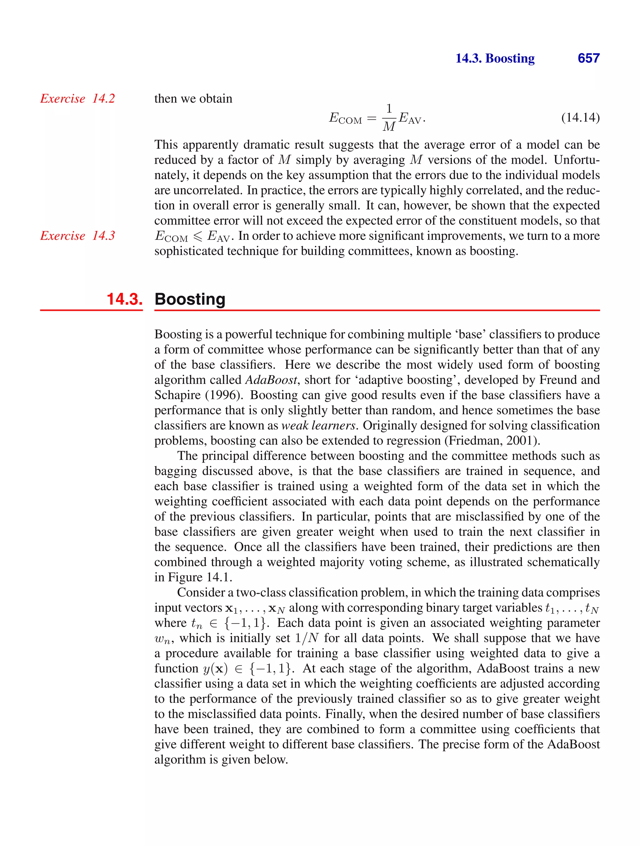
This document provides a list of books published in the Information Science and Statistics series edited by Michael Jordan, Jon Kleinberg, and Bernhard Schölkopf. The list includes books on topics such as time series analysis, pattern recognition, probabilistic networks, Monte Carlo methods, neural networks, quality improvement charts, Bayesian networks, computer intrusion detection, combinatorial optimization, and statistical learning theory. It also provides biographical information about Christopher Bishop, the author of the book "Pattern Recognition and Machine Learning", which is part of this series.


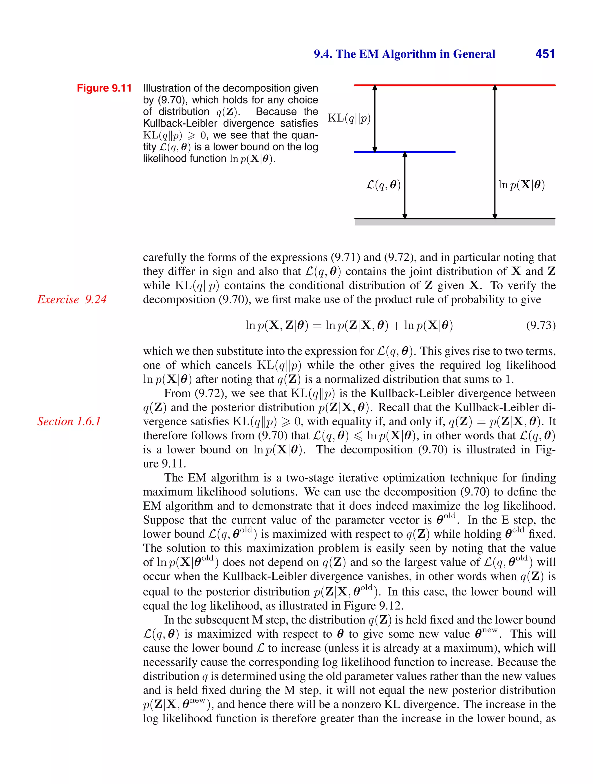
![Mathematical notation
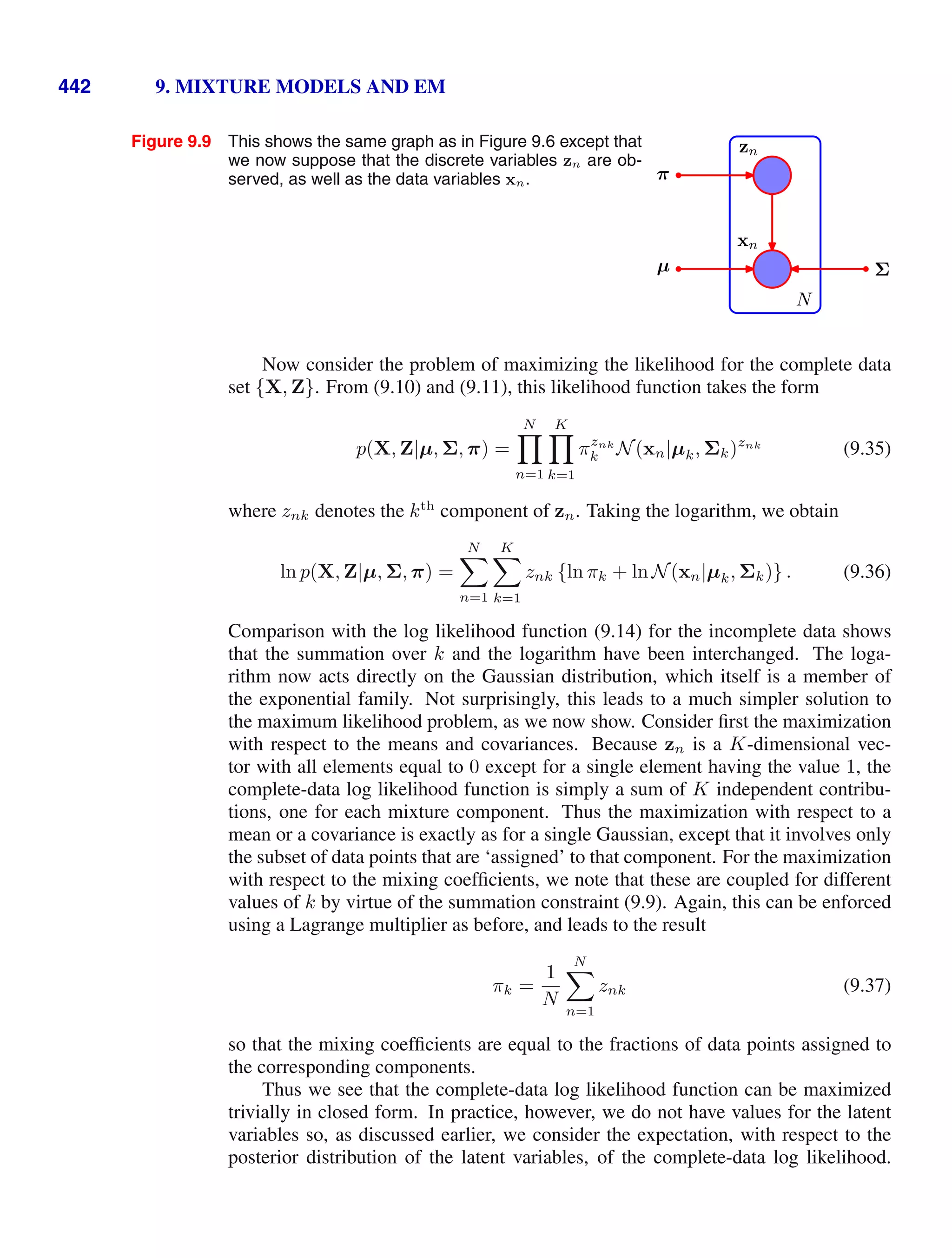
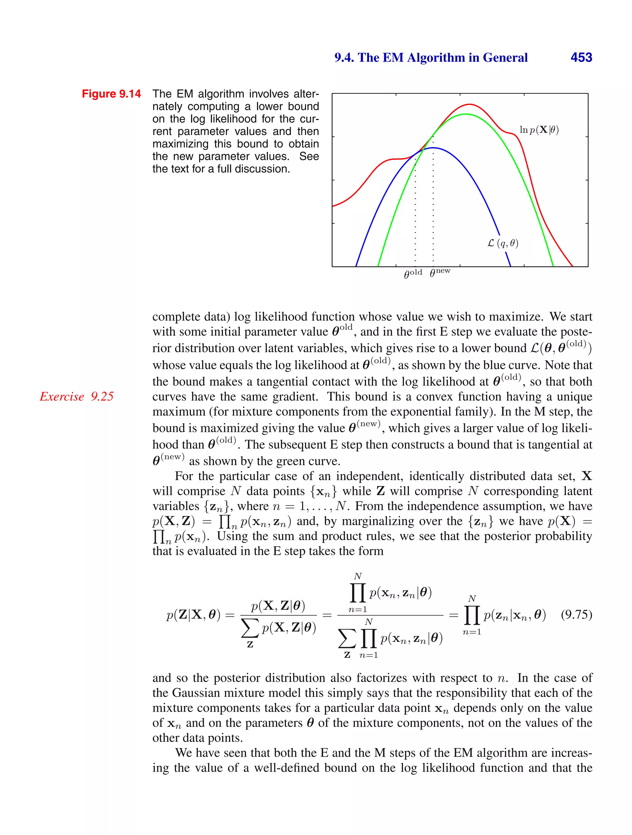
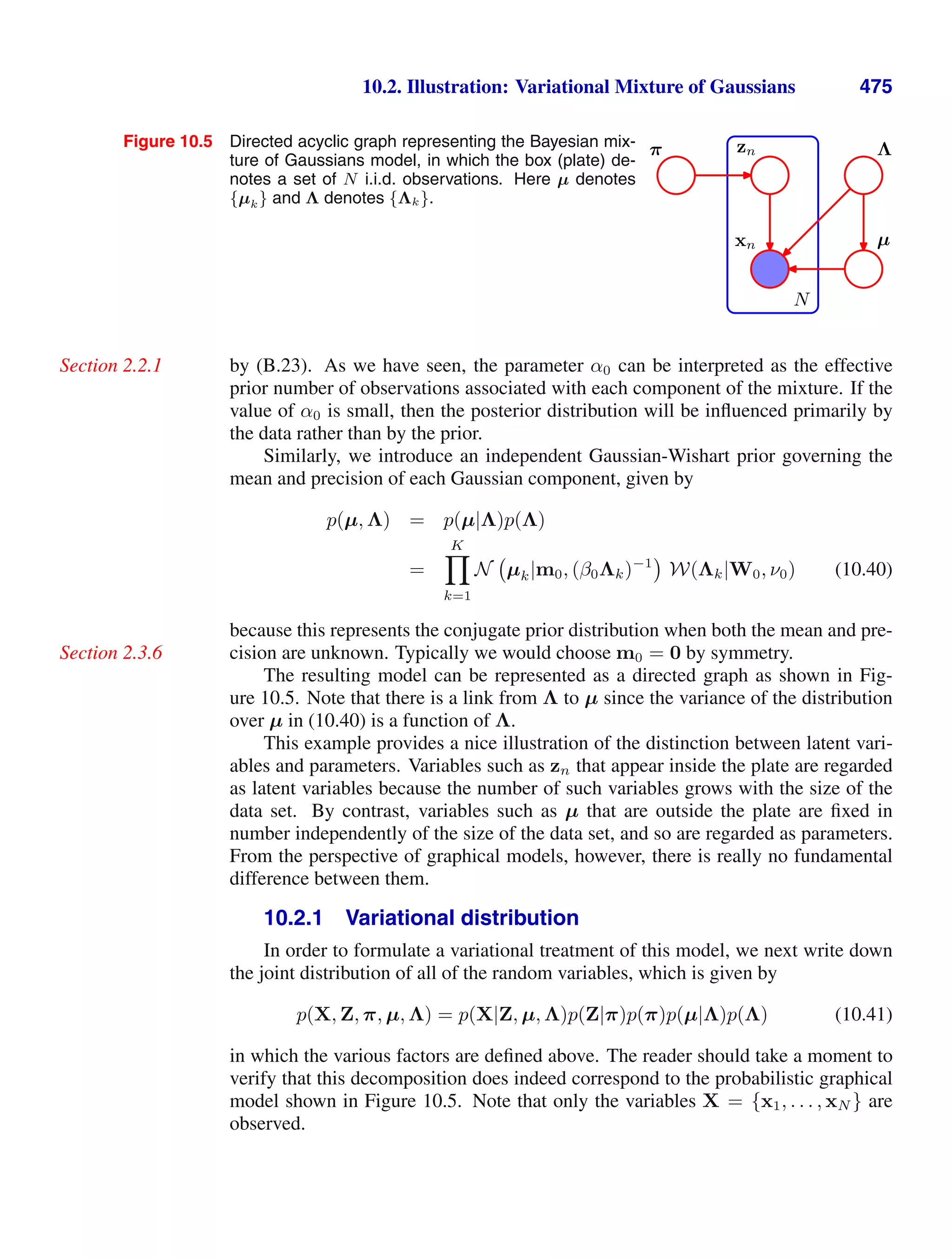
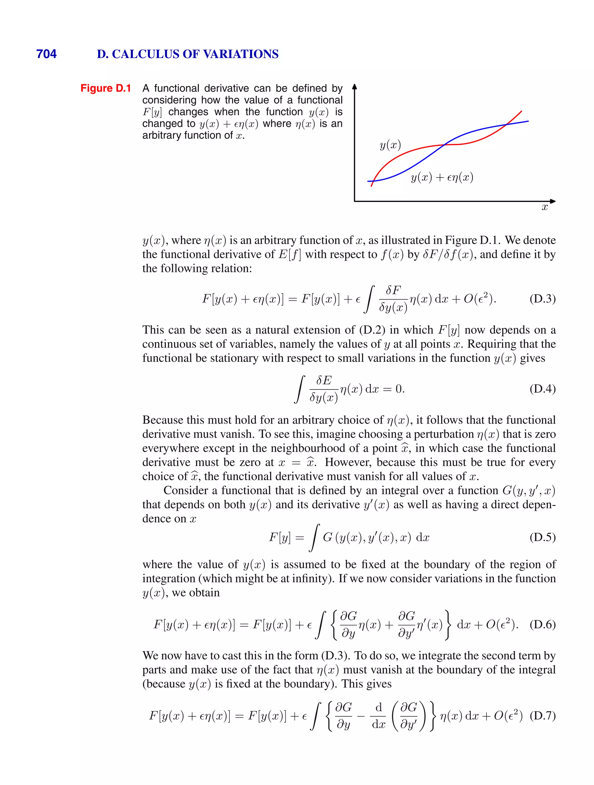
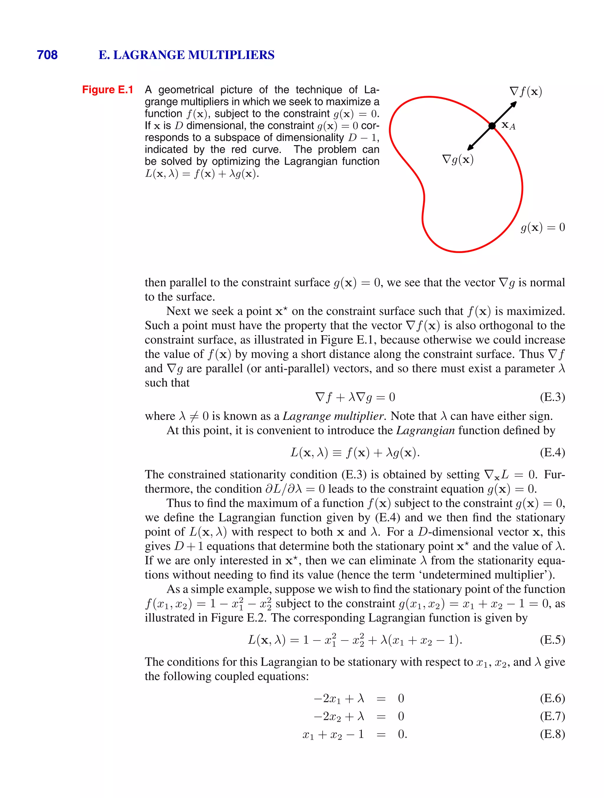
I have tried to keep the mathematical content of the book to the minimum neces-
sary to achieve a proper understanding of the field. However, this minimum level is
nonzero, and it should be emphasized that a good grasp of calculus, linear algebra,
and probability theory is essential for a clear understanding of modern pattern recog-
nition and machine learning techniques. Nevertheless, the emphasis in this book is
on conveying the underlying concepts rather than on mathematical rigour.
I have tried to use a consistent notation throughout the book, although at times
this means departing from some of the conventions used in the corresponding re-
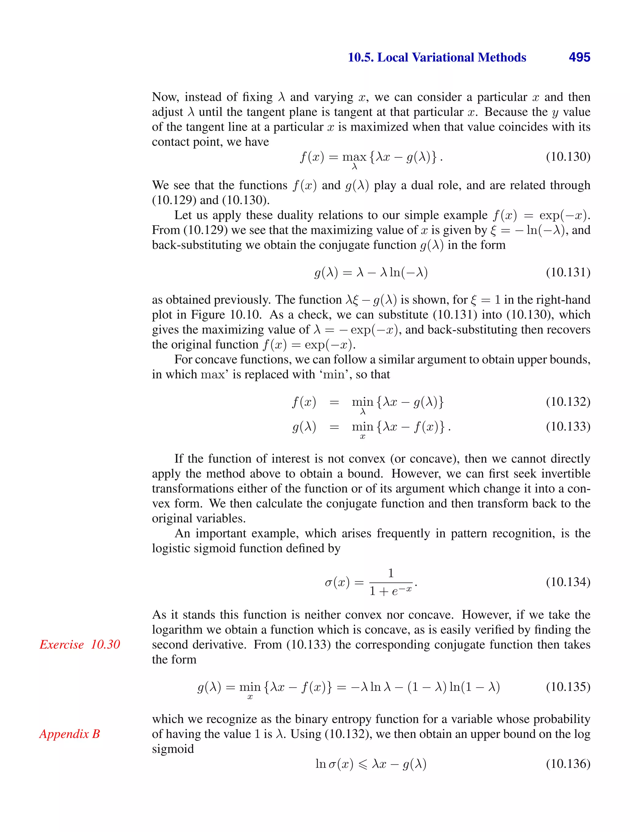
search literature. Vectors are denoted by lower case bold Roman letters such as
x, and all vectors are assumed to be column vectors. A superscript T denotes the
transpose of a matrix or vector, so that xT
will be a row vector. Uppercase bold
roman letters, such as M, denote matrices. The notation (w1, . . . , wM ) denotes a
row vector with M elements, while the corresponding column vector is written as
w = (w1, . . . , wM )T
.
The notation [a, b] is used to denote the closed interval from a to b, that is the
interval including the values a and b themselves, while (a, b) denotes the correspond-
ing open interval, that is the interval excluding a and b. Similarly, [a, b) denotes an
interval that includes a but excludes b. For the most part, however, there will be
little need to dwell on such refinements as whether the end points of an interval are
included or not.
The M × M identity matrix (also known as the unit matrix) is denoted IM ,
which will be abbreviated to I where there is no ambiguity about it dimensionality.
It has elements Iij that equal 1 if i = j and 0 if i = j.
A functional is denoted f[y] where y(x) is some function. The concept of a
functional is discussed in Appendix D.
The notation g(x) = O(f(x)) denotes that |f(x)/g(x)| is bounded as x → ∞.
For instance if g(x) = 3x2
+ 2, then g(x) = O(x2
).
The expectation of a function f(x, y) with respect to a random variable x is de-
noted by Ex[f(x, y)]. In situations where there is no ambiguity as to which variable
is being averaged over, this will be simplified by omitting the suffix, for instance
xi](https://image.slidesharecdn.com/bishop-patternrecognitionandmachinelearning-230316082240-9af1cdaa/75/Bishop-Pattern-Recognition-and-Machine-Learning-pdf-9-2048.jpg)
![xii MATHEMATICAL NOTATION
E[x]. If the distribution of x is conditioned on another variable z, then the corre-
sponding conditional expectation will be written Ex[f(x)|z]. Similarly, the variance
is denoted var[f(x)], and for vector variables the covariance is written cov[x, y]. We
shall also use cov[x] as a shorthand notation for cov[x, x]. The concepts of expecta-
tions and covariances are introduced in Section 1.2.2.
If we have N values x1, . . . , xN of a D-dimensional vector x = (x1, . . . , xD)T
,
we can combine the observations into a data matrix X in which the nth
row of X
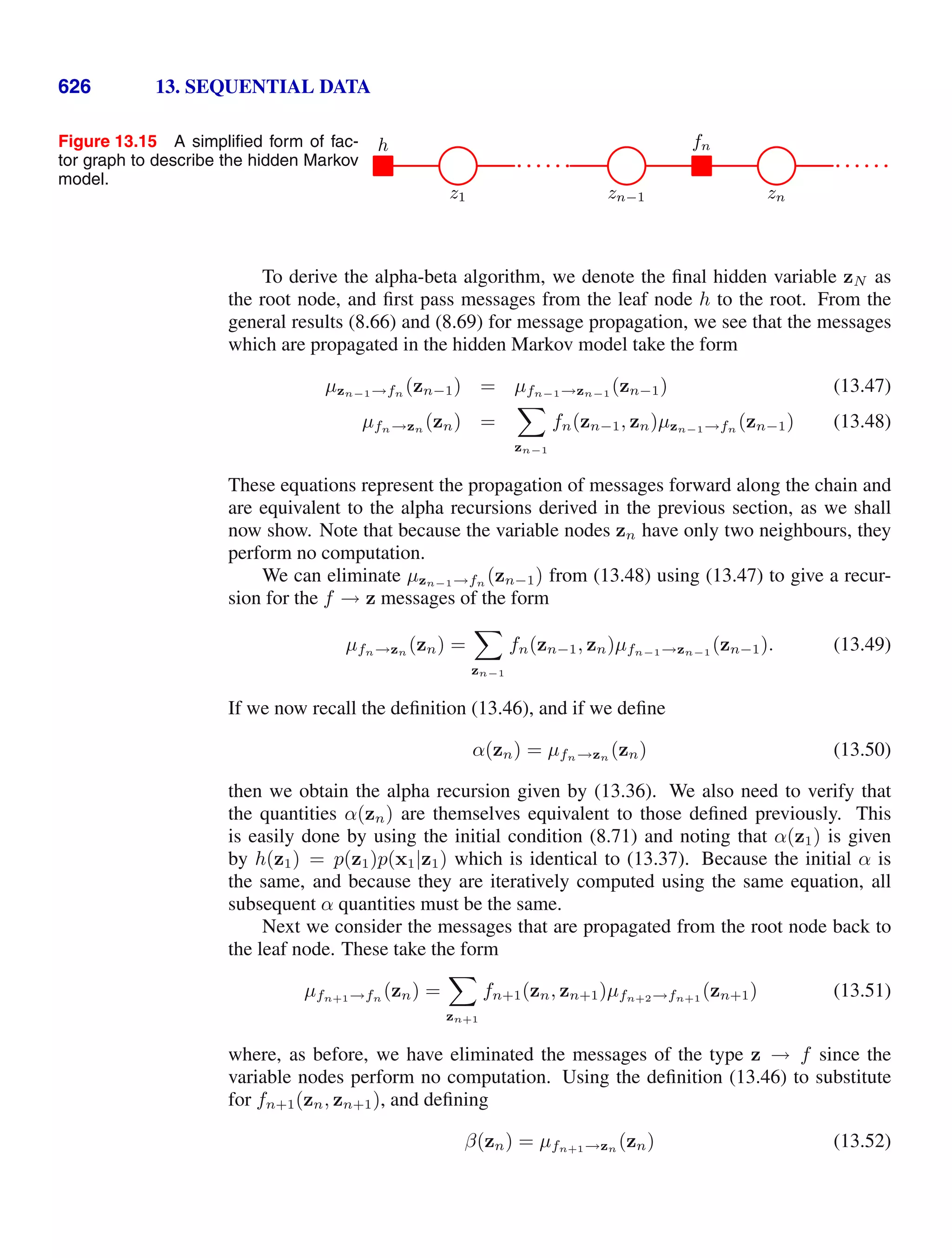
corresponds to the row vector xT
n. Thus the n, i element of X corresponds to the
ith
element of the nth
observation xn. For the case of one-dimensional variables we
shall denote such a matrix by x, which is a column vector whose nth
element is xn.
Note that x (which has dimensionality N) uses a different typeface to distinguish it
from x (which has dimensionality D).](https://image.slidesharecdn.com/bishop-patternrecognitionandmachinelearning-230316082240-9af1cdaa/75/Bishop-Pattern-Recognition-and-Machine-Learning-pdf-10-2048.jpg)


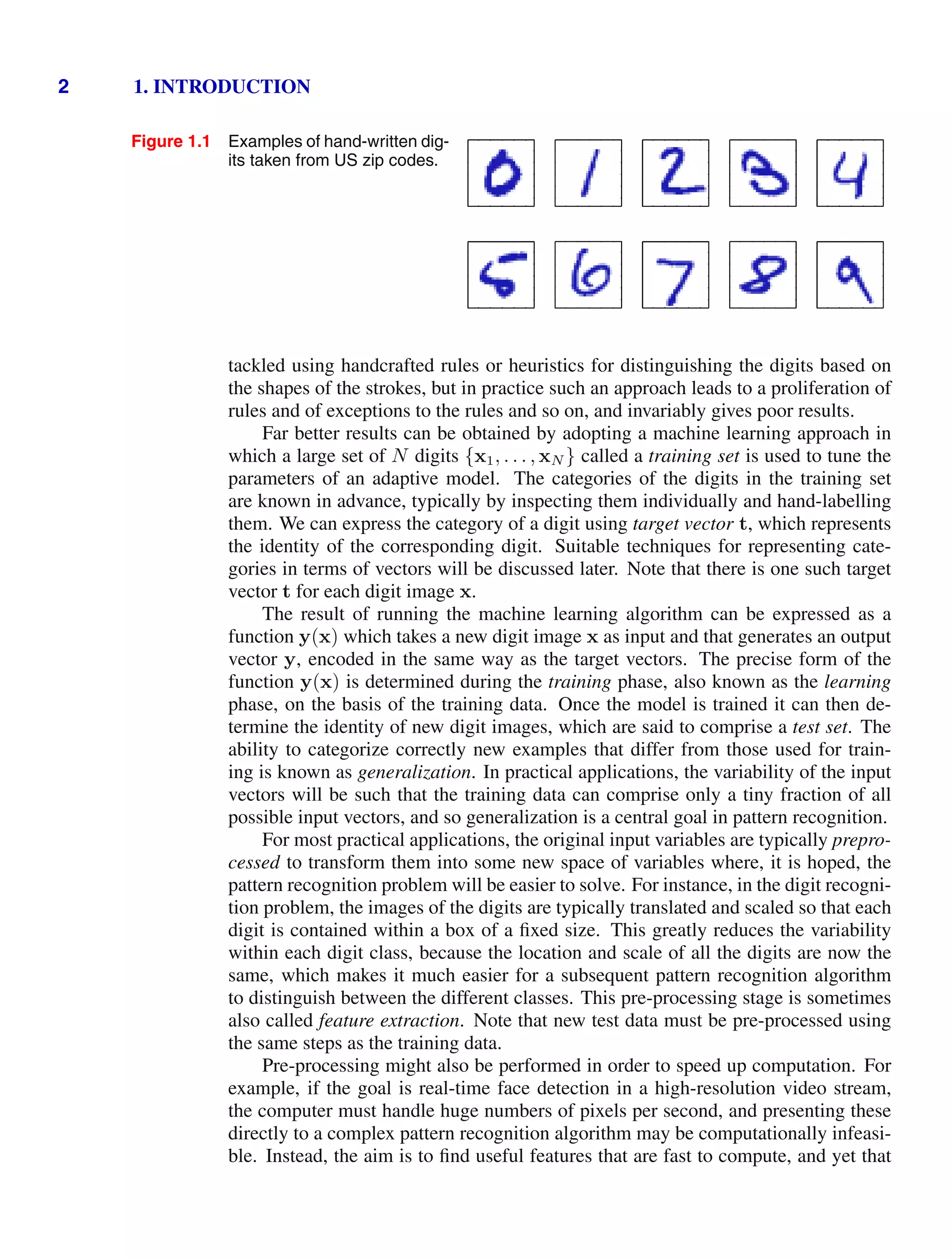
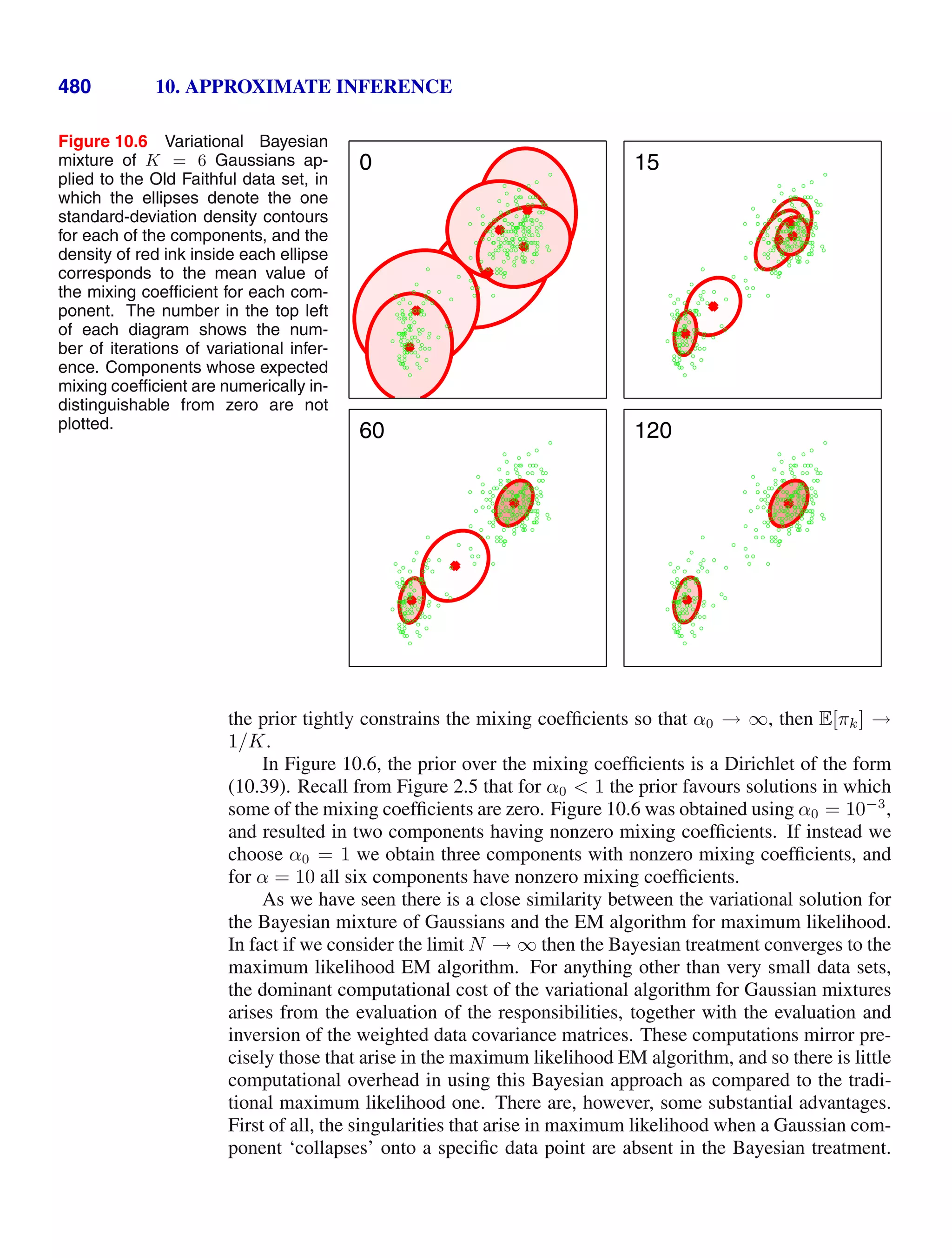
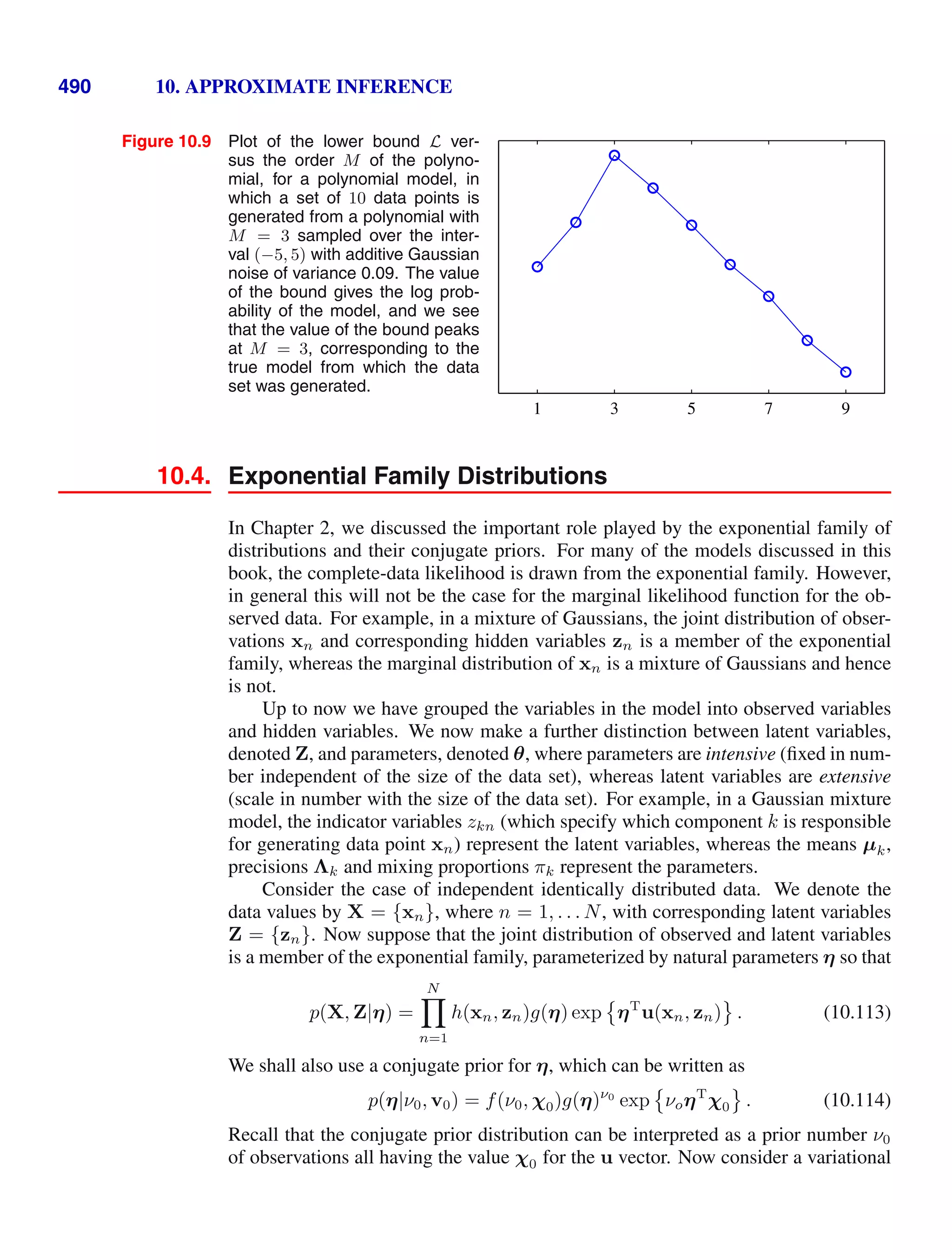
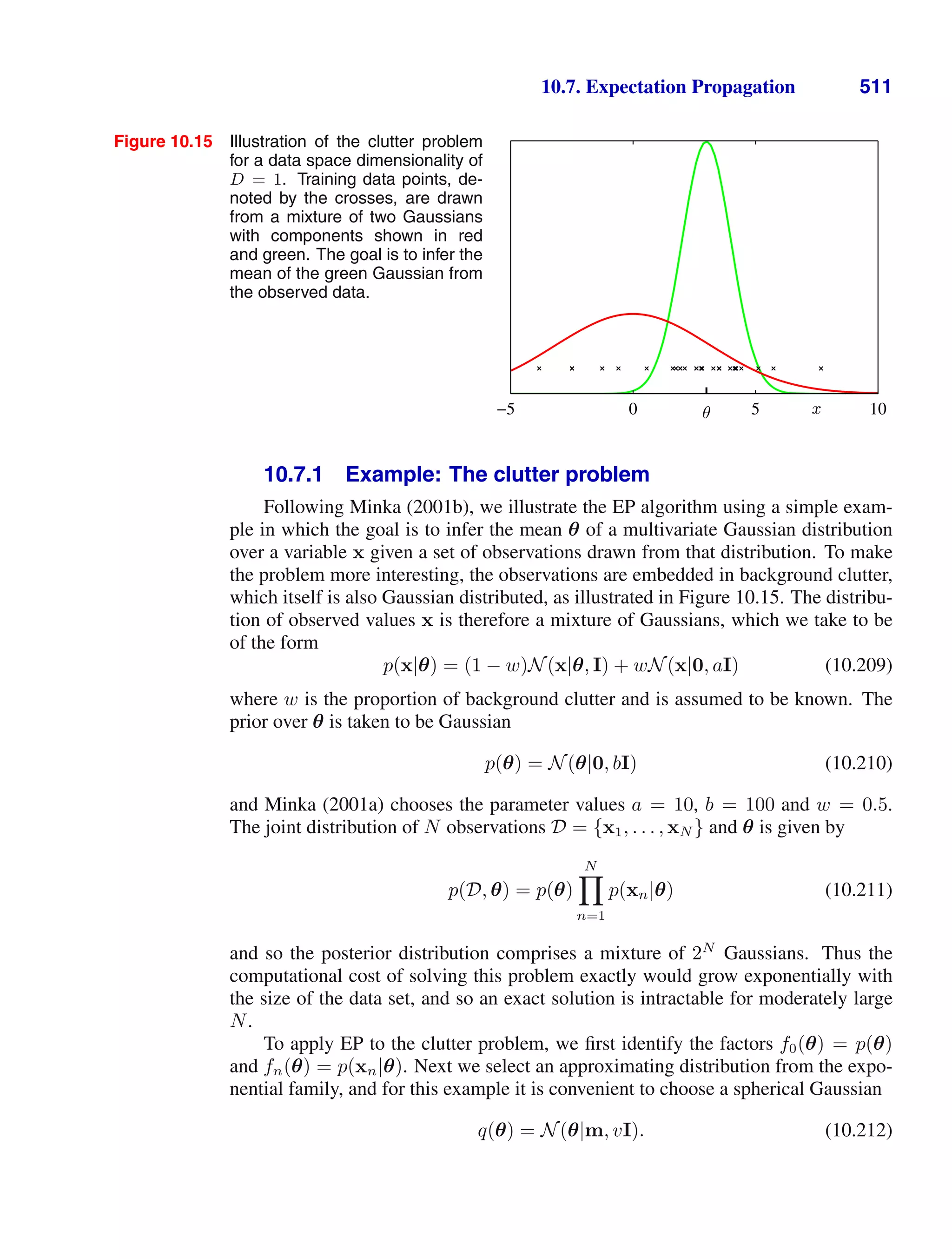
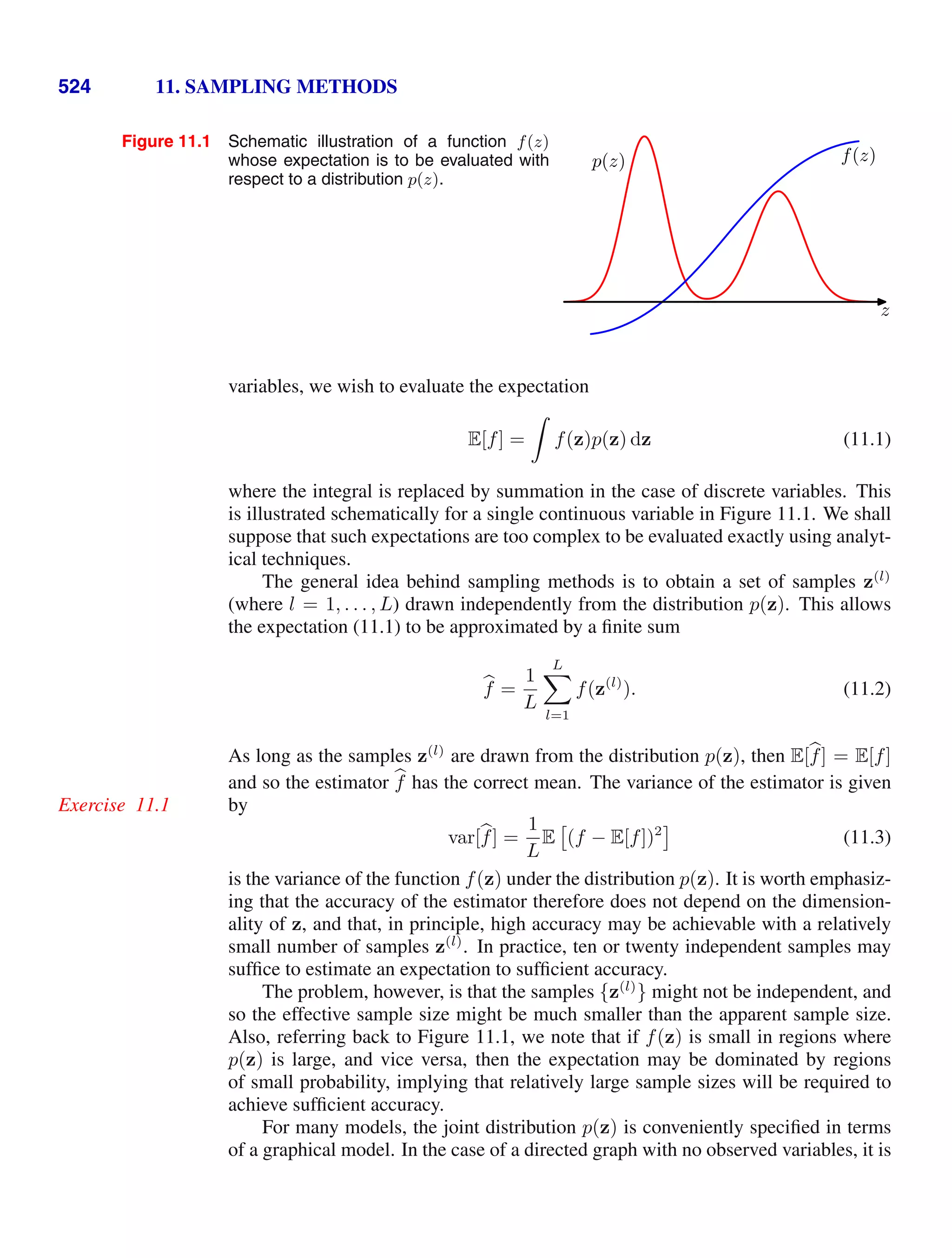
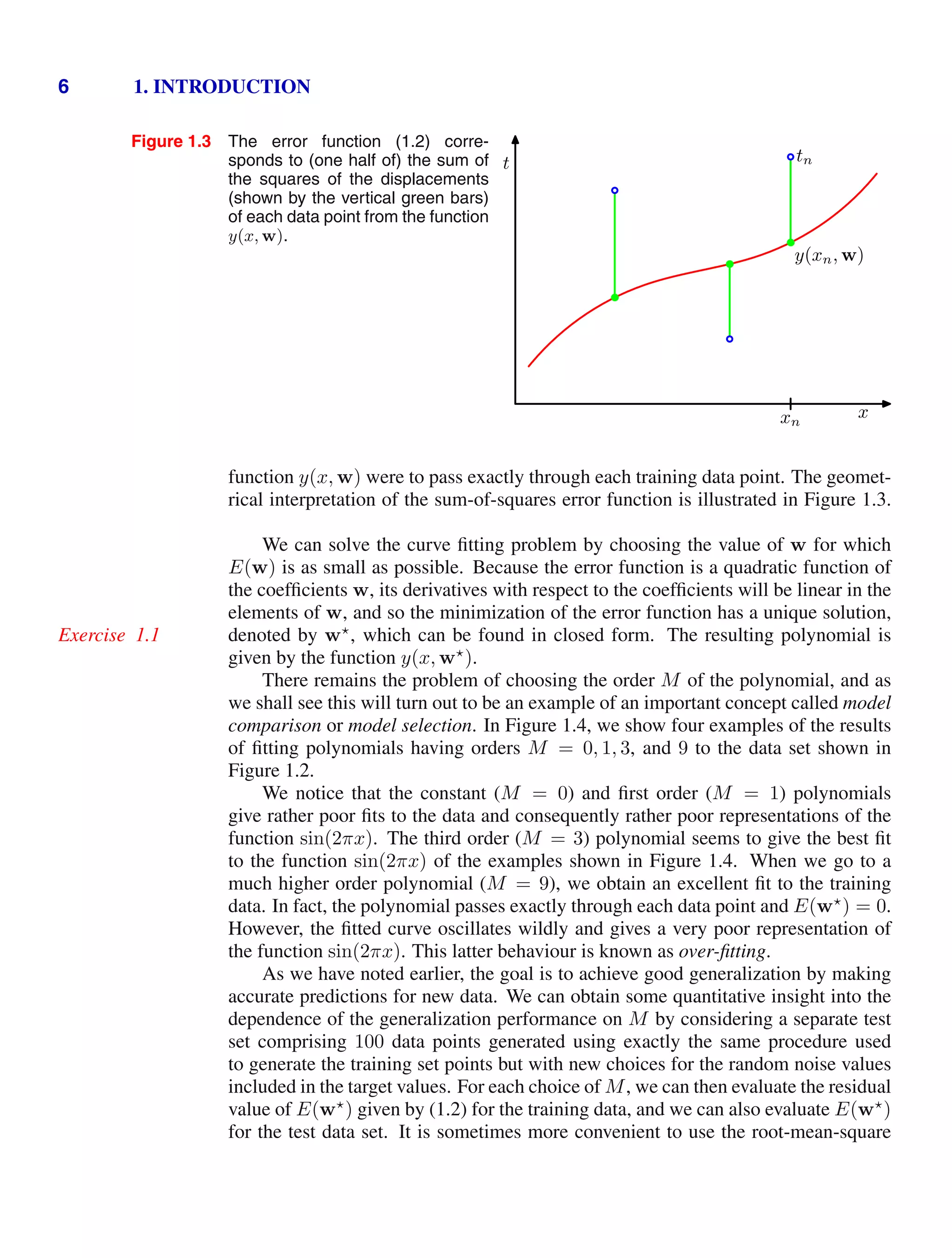
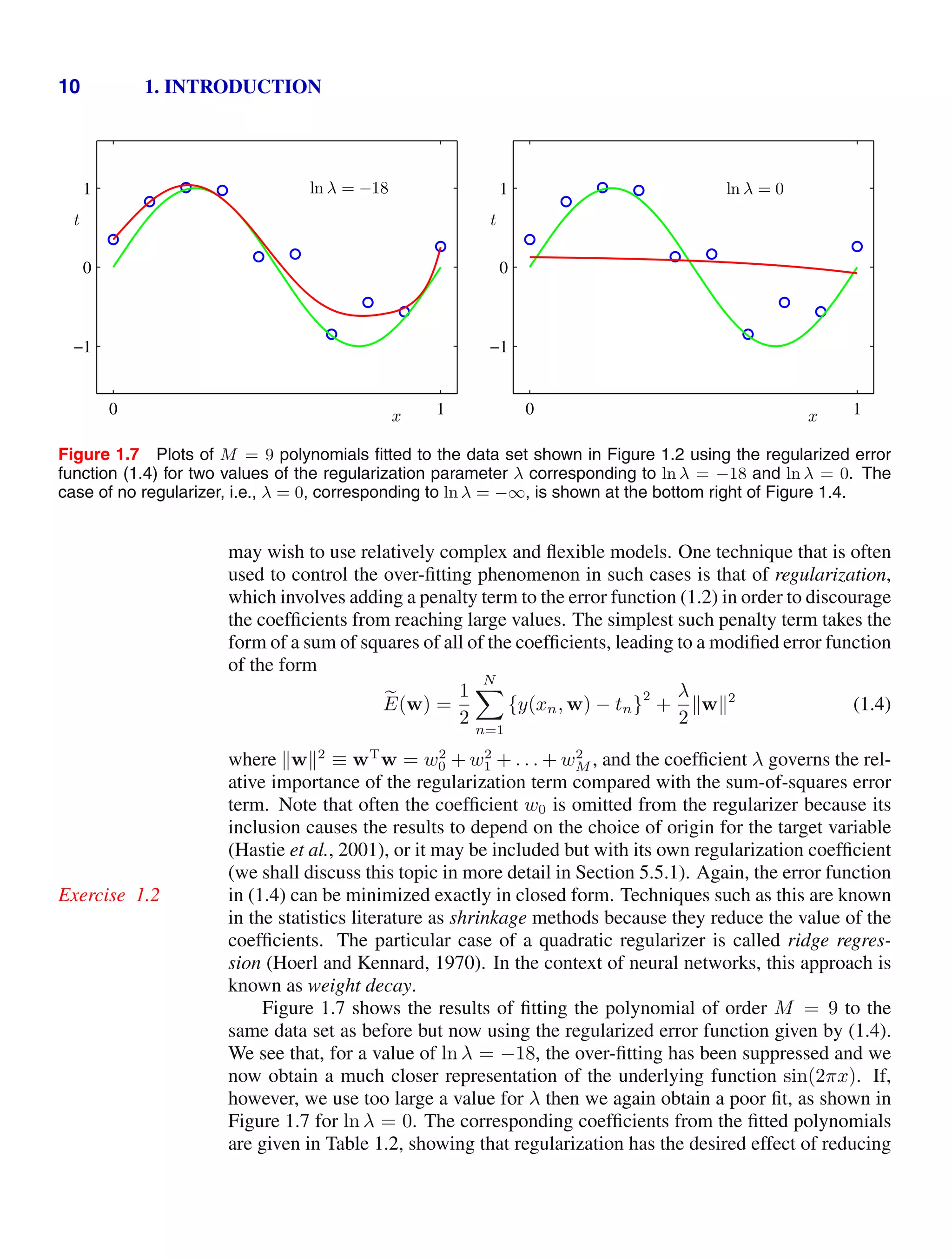
![4 1. INTRODUCTION
Figure 1.2 Plot of a training data set of N =
10 points, shown as blue circles,
each comprising an observation
of the input variable x along with
the corresponding target variable
t. The green curve shows the
function sin(2πx) used to gener-
ate the data. Our goal is to pre-
dict the value of t for some new
value of x, without knowledge of
the green curve.
x
t
0 1
−1
0
1
detailed treatment lies beyond the scope of this book.
Although each of these tasks needs its own tools and techniques, many of the
key ideas that underpin them are common to all such problems. One of the main
goals of this chapter is to introduce, in a relatively informal way, several of the most
important of these concepts and to illustrate them using simple examples. Later in
the book we shall see these same ideas re-emerge in the context of more sophisti-
cated models that are applicable to real-world pattern recognition applications. This
chapter also provides a self-contained introduction to three important tools that will
be used throughout the book, namely probability theory, decision theory, and infor-
mation theory. Although these might sound like daunting topics, they are in fact
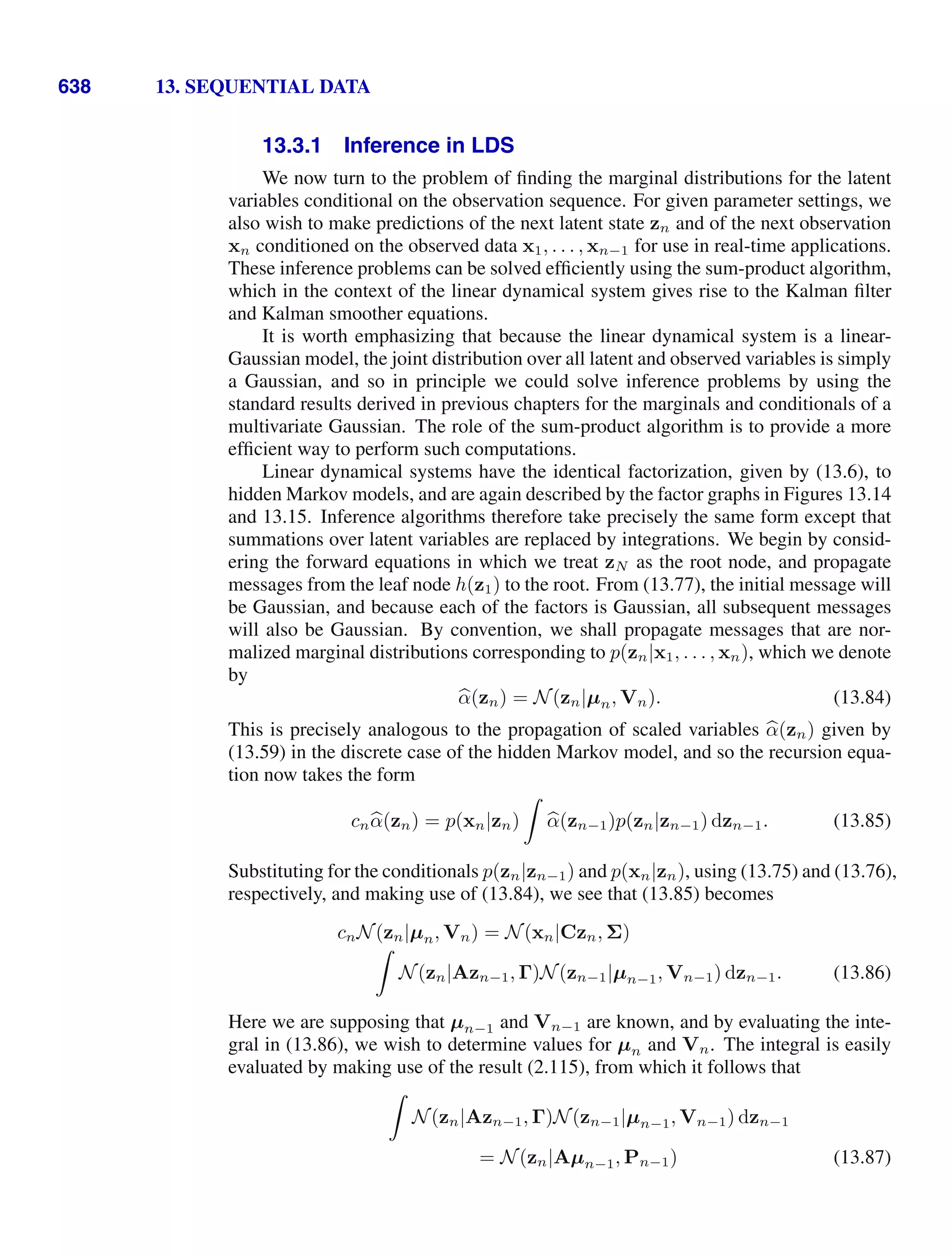
straightforward, and a clear understanding of them is essential if machine learning
techniques are to be used to best effect in practical applications.
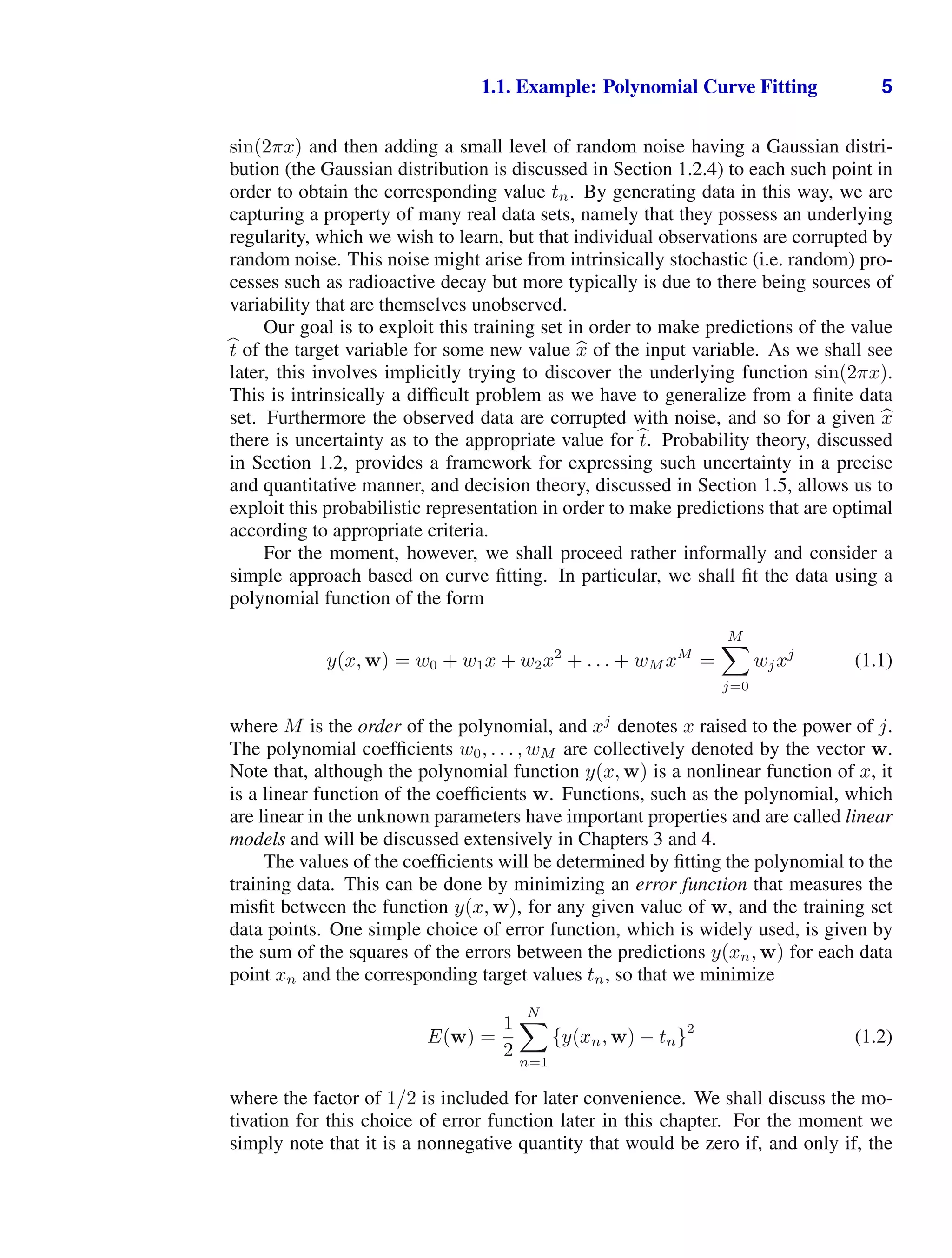
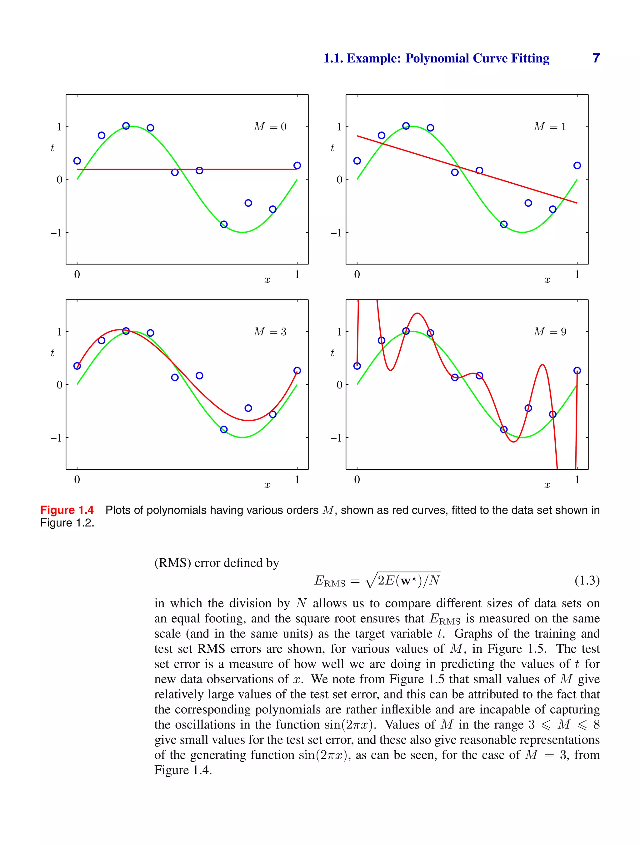
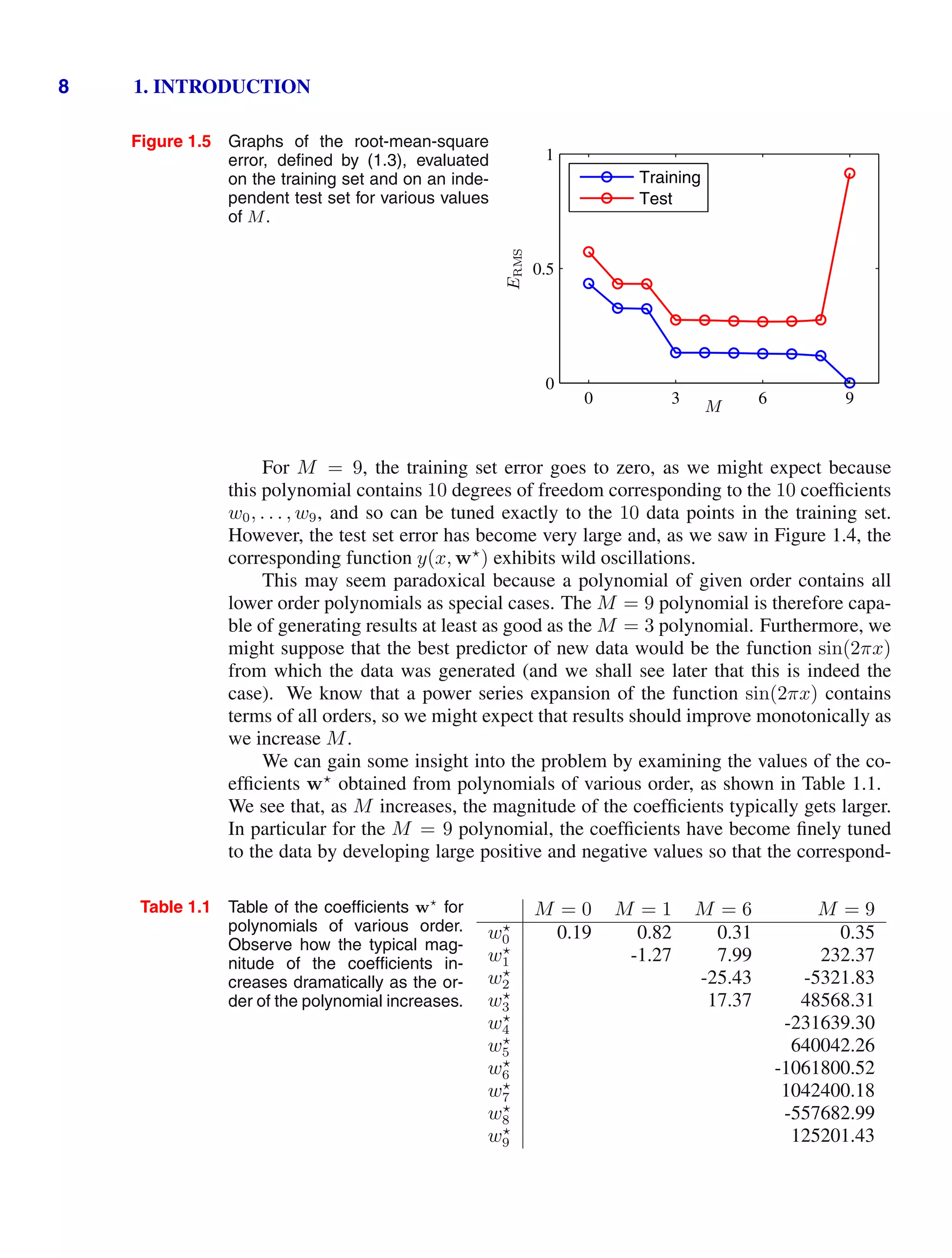
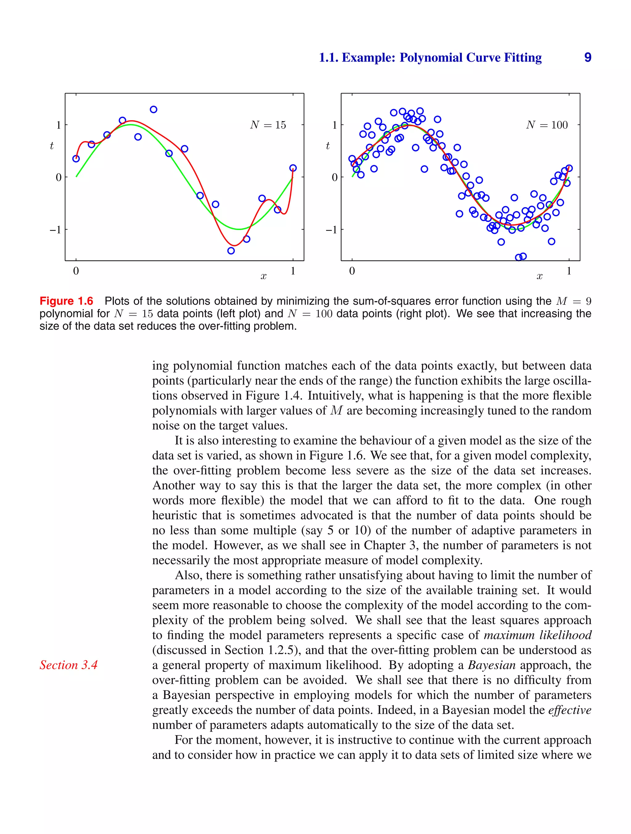
1.1. Example: Polynomial Curve Fitting
We begin by introducing a simple regression problem, which we shall use as a run-
ning example throughout this chapter to motivate a number of key concepts. Sup-
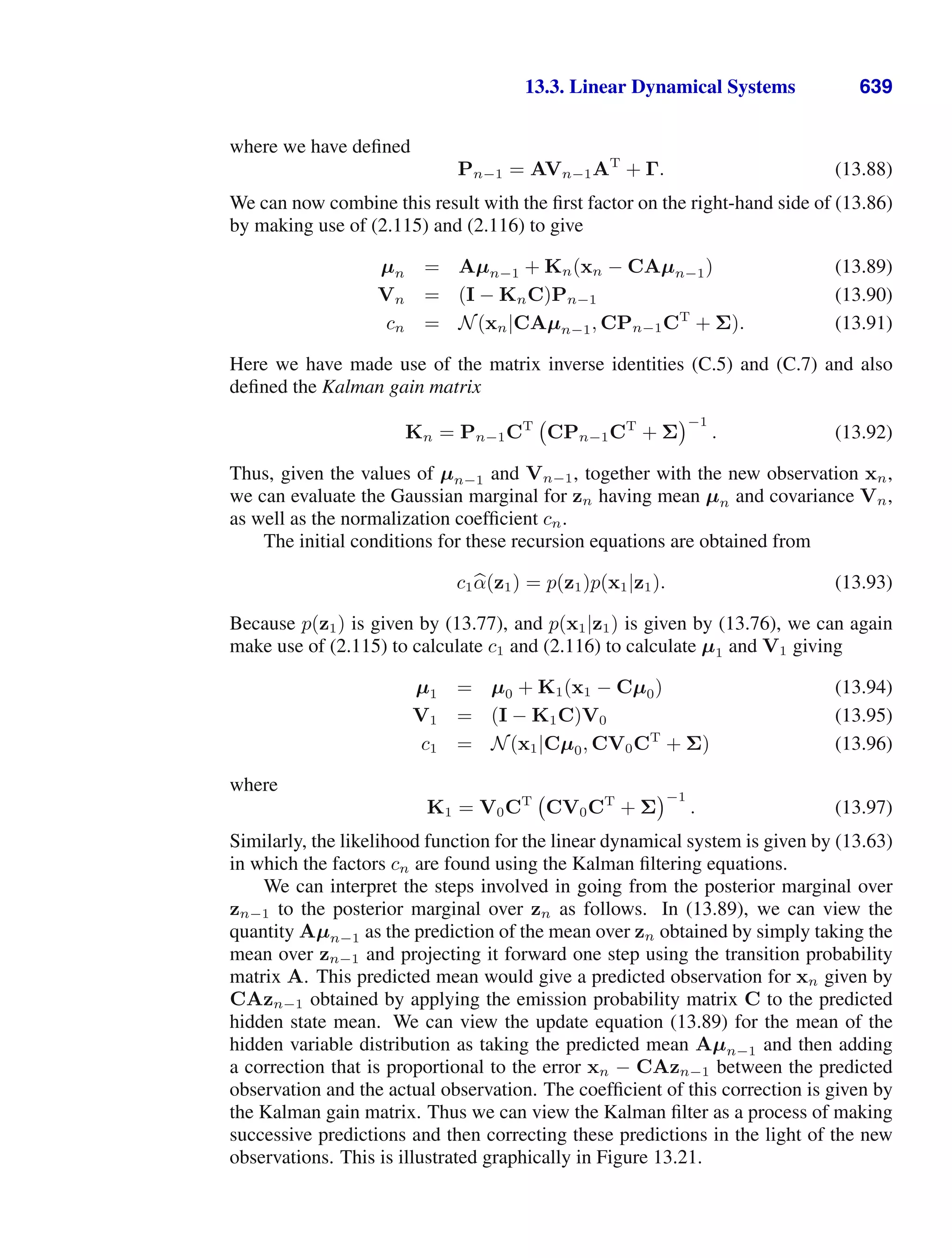
pose we observe a real-valued input variable x and we wish to use this observation to
predict the value of a real-valued target variable t. For the present purposes, it is in-
structive to consider an artificial example using synthetically generated data because
we then know the precise process that generated the data for comparison against any
learned model. The data for this example is generated from the function sin(2πx)
with random noise included in the target values, as described in detail in Appendix A.
Now suppose that we are given a training set comprising N observations of x,
written x ≡ (x1, . . . , xN )T
, together with corresponding observations of the values
of t, denoted t ≡ (t1, . . . , tN )T
. Figure 1.2 shows a plot of a training set comprising
N = 10 data points. The input data set x in Figure 1.2 was generated by choos-
ing values of xn, for n = 1, . . . , N, spaced uniformly in range [0, 1], and the target
data set t was obtained by first computing the corresponding values of the function](https://image.slidesharecdn.com/bishop-patternrecognitionandmachinelearning-230316082240-9af1cdaa/75/Bishop-Pattern-Recognition-and-Machine-Learning-pdf-22-2048.jpg)
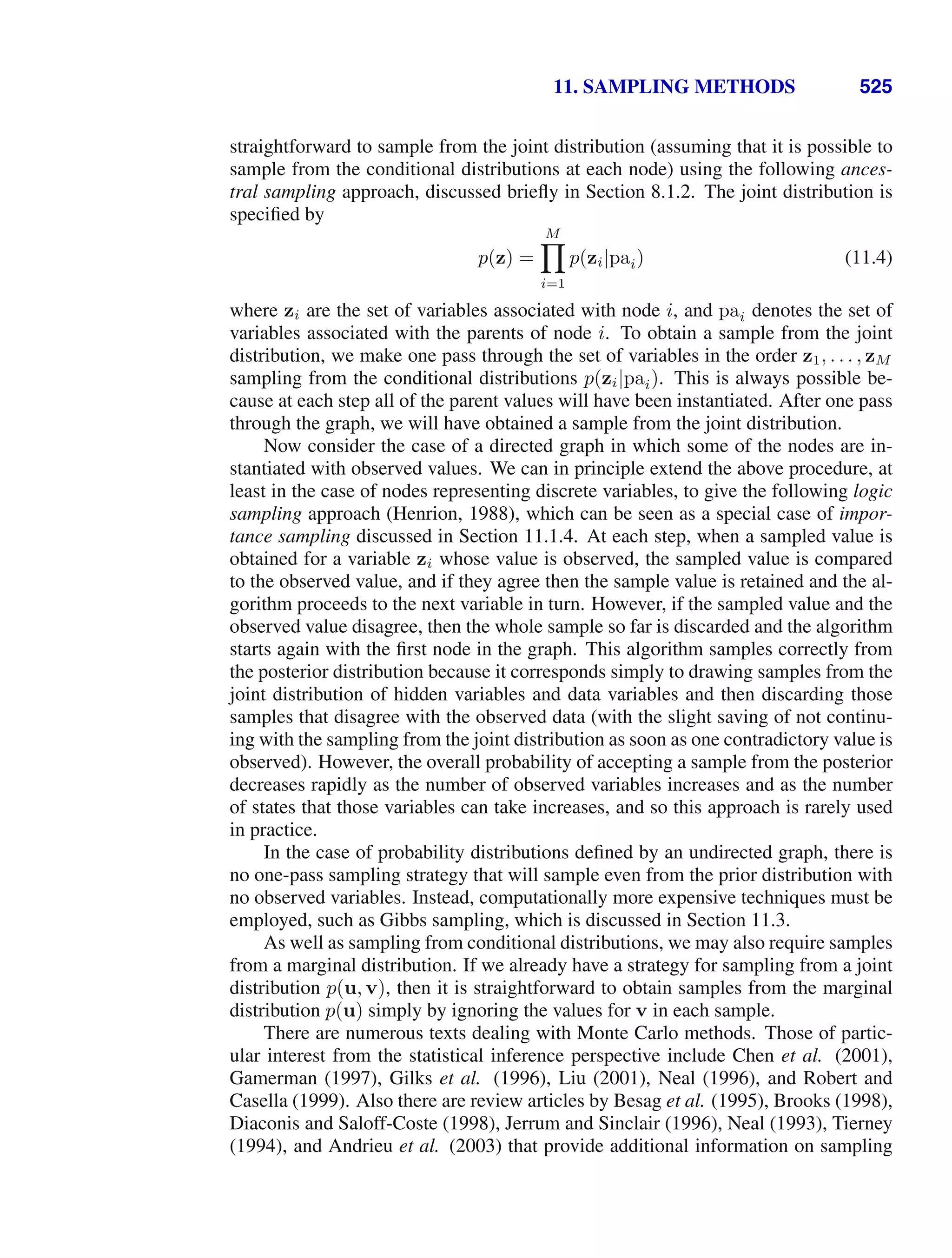
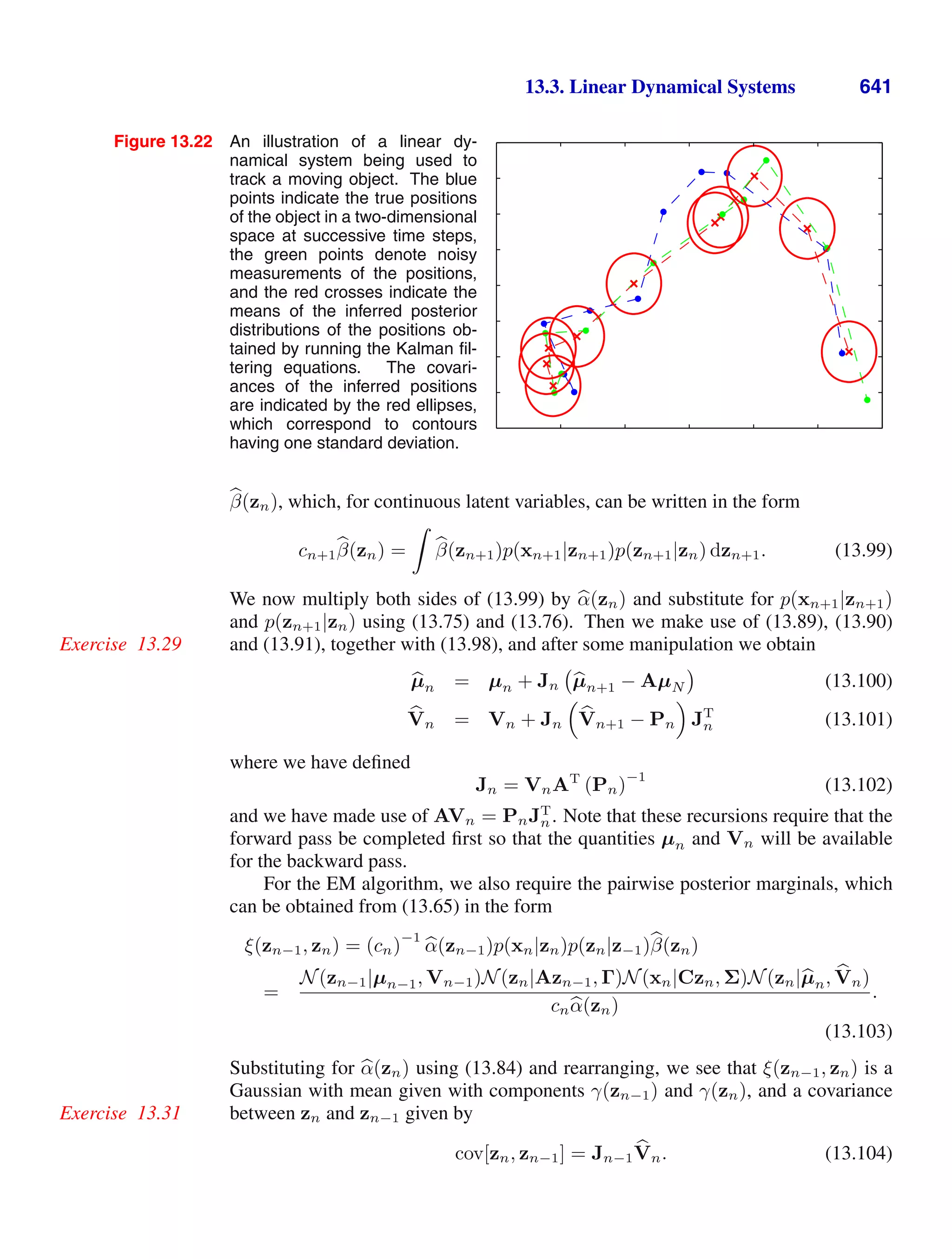
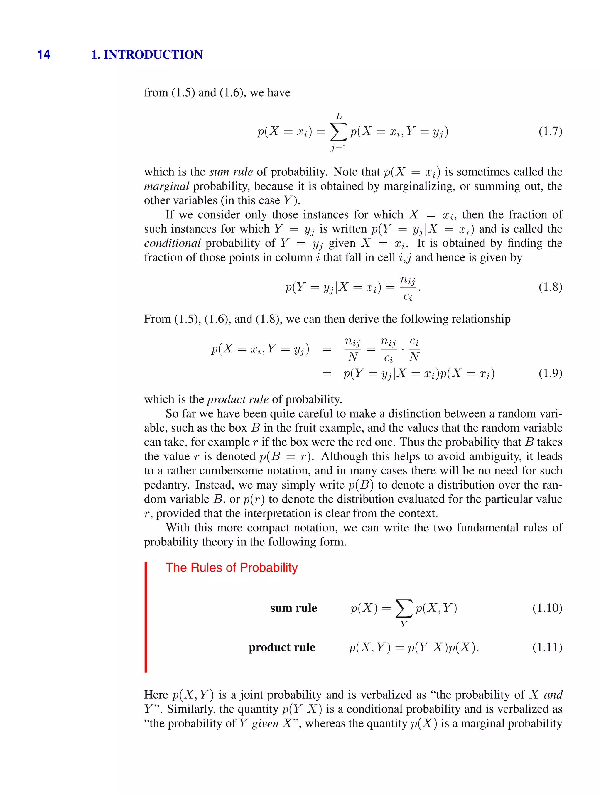
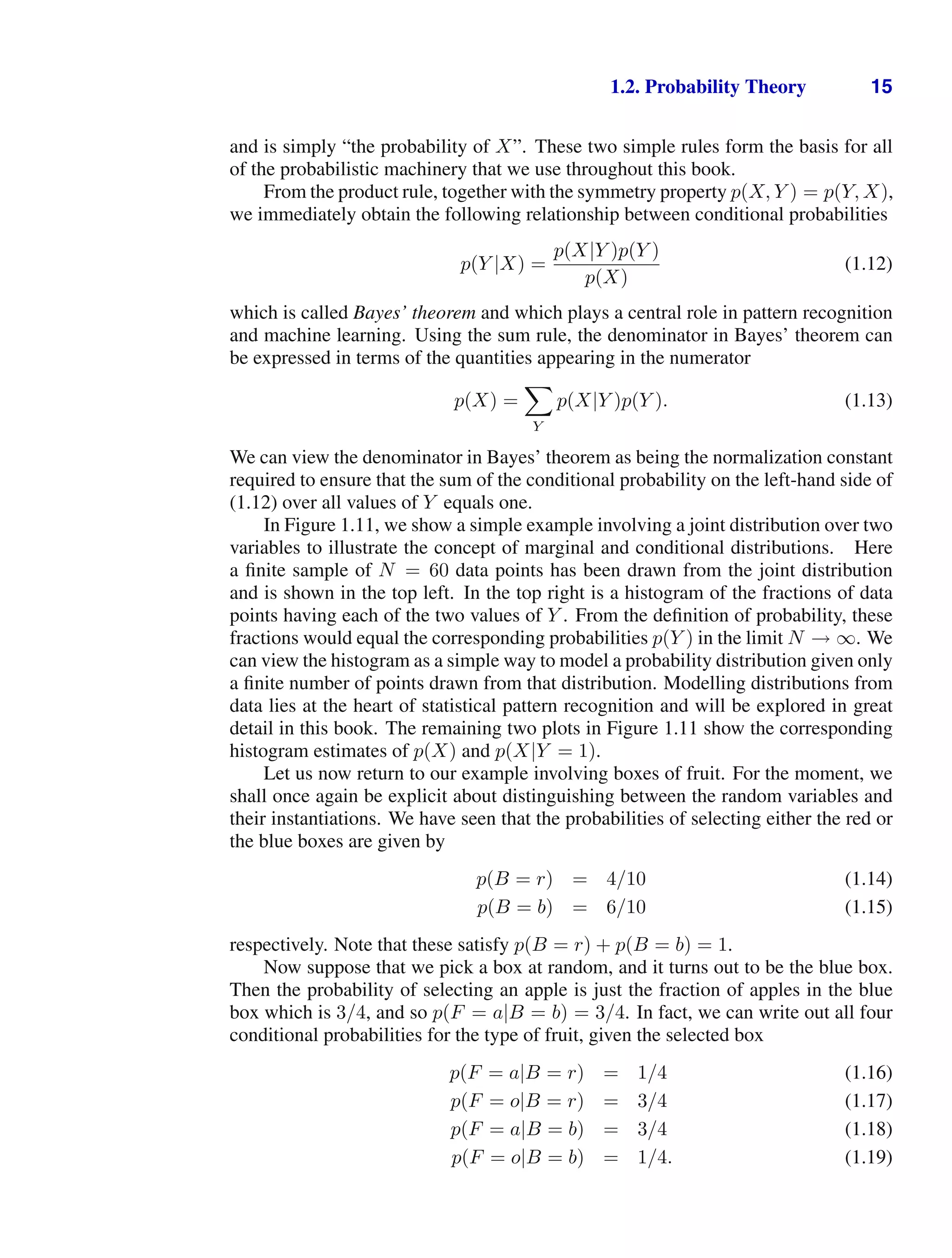
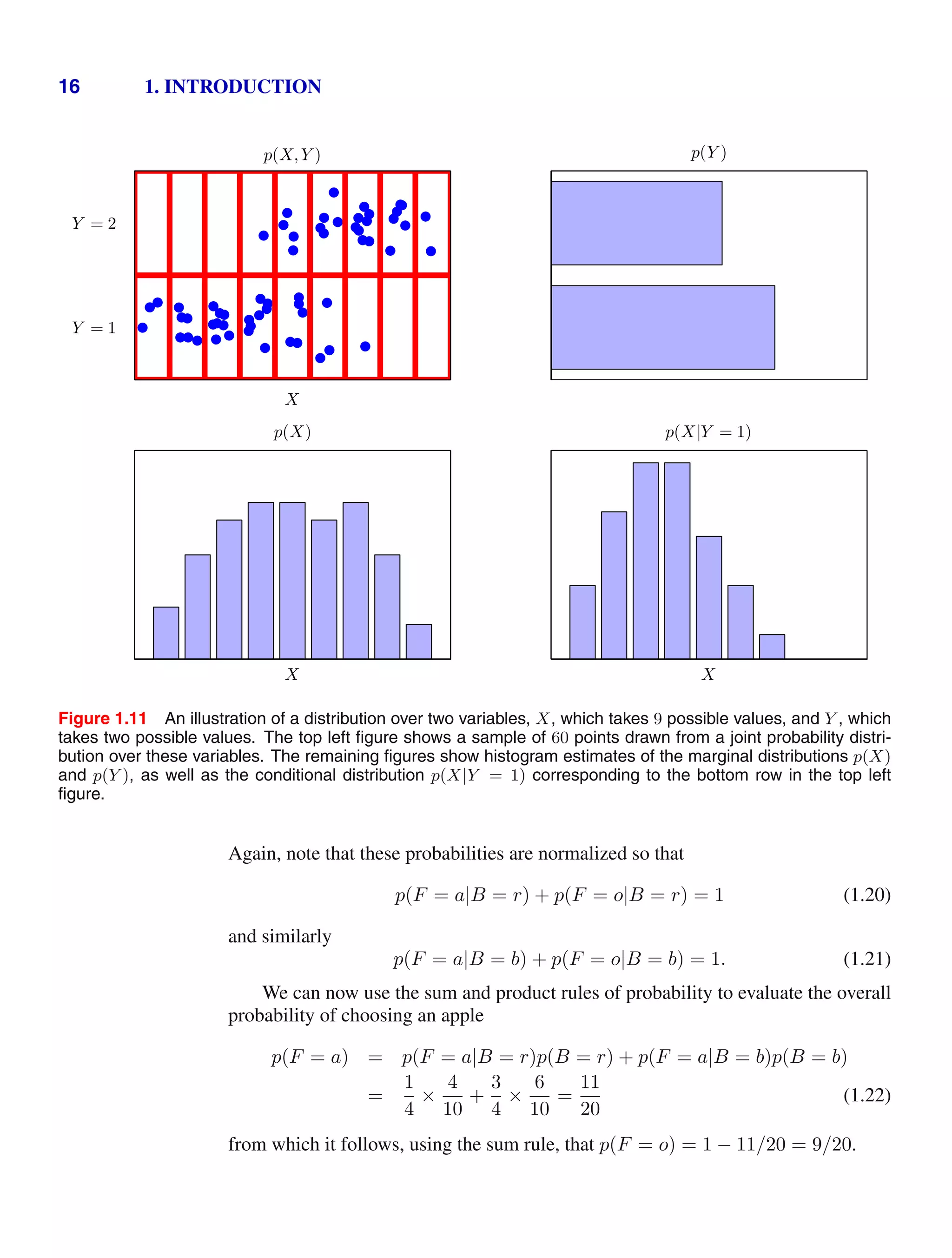
![1.2. Probability Theory 13
Figure 1.10 We can derive the sum and product rules of probability by
considering two random variables, X, which takes the values {xi} where
i = 1, . . . , M, and Y , which takes the values {yj} where j = 1, . . . , L.
In this illustration we have M = 5 and L = 3. If we consider a total
number N of instances of these variables, then we denote the number
of instances where X = xi and Y = yj by nij, which is the number of
points in the corresponding cell of the array. The number of points in
column i, corresponding to X = xi, is denoted by ci, and the number of
points in row j, corresponding to Y = yj, is denoted by rj.
}
}
ci
rj
yj
xi
nij
and the probability of selecting the blue box is 6/10. We write these probabilities
as p(B = r) = 4/10 and p(B = b) = 6/10. Note that, by definition, probabilities
must lie in the interval [0, 1]. Also, if the events are mutually exclusive and if they
include all possible outcomes (for instance, in this example the box must be either
red or blue), then we see that the probabilities for those events must sum to one.
We can now ask questions such as: “what is the overall probability that the se-
lection procedure will pick an apple?”, or “given that we have chosen an orange,
what is the probability that the box we chose was the blue one?”. We can answer
questions such as these, and indeed much more complex questions associated with
problems in pattern recognition, once we have equipped ourselves with the two el-
ementary rules of probability, known as the sum rule and the product rule. Having
obtained these rules, we shall then return to our boxes of fruit example.
In order to derive the rules of probability, consider the slightly more general ex-
ample shown in Figure 1.10 involving two random variables X and Y (which could
for instance be the Box and Fruit variables considered above). We shall suppose that
X can take any of the values xi where i = 1, . . . , M, and Y can take the values yj
where j = 1, . . . , L. Consider a total of N trials in which we sample both of the
variables X and Y , and let the number of such trials in which X = xi and Y = yj
be nij. Also, let the number of trials in which X takes the value xi (irrespective
of the value that Y takes) be denoted by ci, and similarly let the number of trials in
which Y takes the value yj be denoted by rj.
The probability that X will take the value xi and Y will take the value yj is
written p(X = xi, Y = yj) and is called the joint probability of X = xi and
Y = yj. It is given by the number of points falling in the cell i,j as a fraction of the
total number of points, and hence
p(X = xi, Y = yj) =
nij
N
. (1.5)
Here we are implicitly considering the limit N → ∞. Similarly, the probability that
X takes the value xi irrespective of the value of Y is written as p(X = xi) and is
given by the fraction of the total number of points that fall in column i, so that
p(X = xi) =
ci
N
. (1.6)
Because the number of instances in column i in Figure 1.10 is just the sum of the
number of instances in each cell of that column, we have ci =
j nij and therefore,](https://image.slidesharecdn.com/bishop-patternrecognitionandmachinelearning-230316082240-9af1cdaa/75/Bishop-Pattern-Recognition-and-Machine-Learning-pdf-31-2048.jpg)
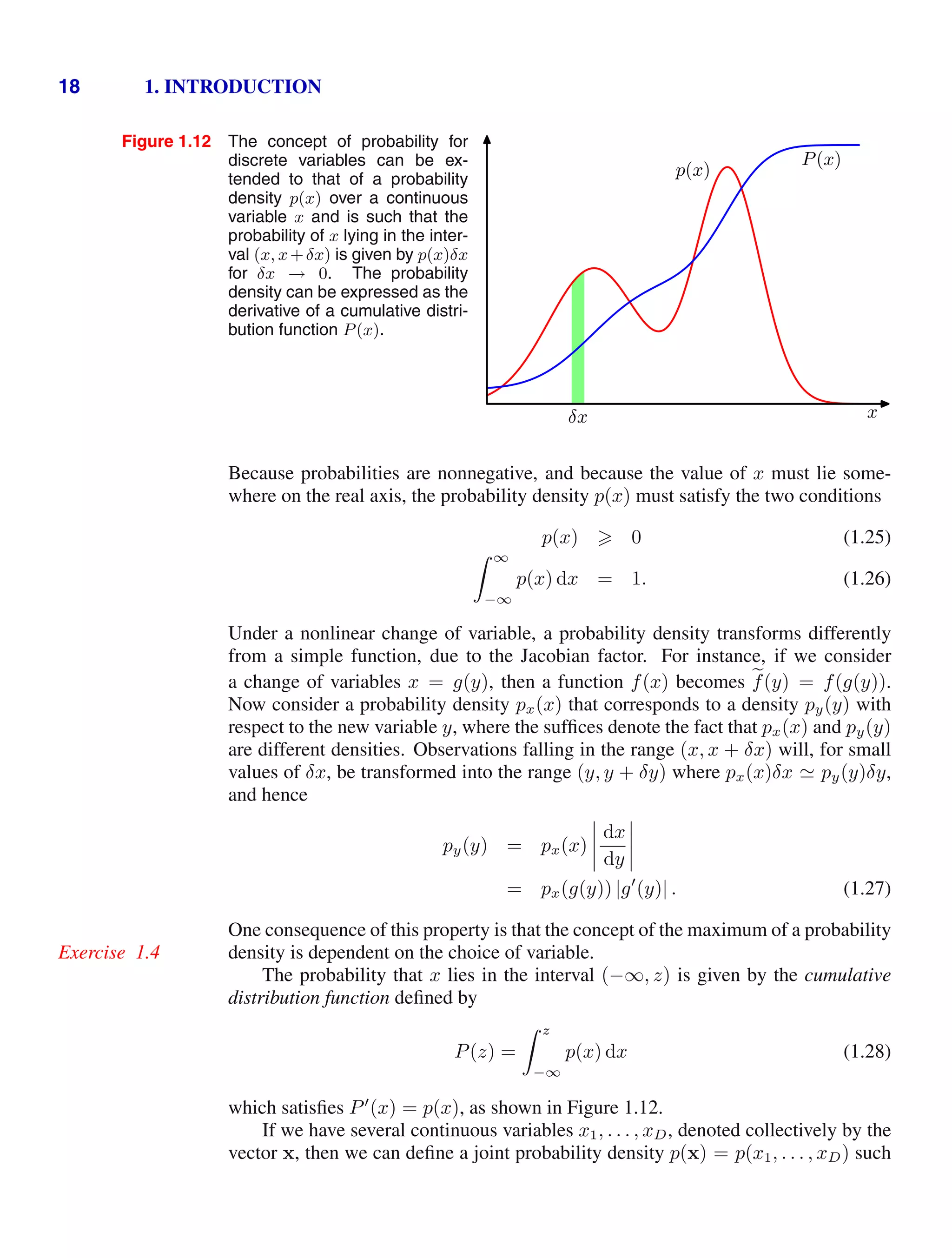
![1.2. Probability Theory 19
that the probability of x falling in an infinitesimal volume δx containing the point x
is given by p(x)δx. This multivariate probability density must satisfy
p(x) 0 (1.29)
p(x) dx = 1 (1.30)
in which the integral is taken over the whole of x space. We can also consider joint
probability distributions over a combination of discrete and continuous variables.
Note that if x is a discrete variable, then p(x) is sometimes called a probability
mass function because it can be regarded as a set of ‘probability masses’ concentrated
at the allowed values of x.
The sum and product rules of probability, as well as Bayes’ theorem, apply
equally to the case of probability densities, or to combinations of discrete and con-
tinuous variables. For instance, if x and y are two real variables, then the sum and
product rules take the form
p(x) =
p(x, y) dy (1.31)
p(x, y) = p(y|x)p(x). (1.32)
A formal justification of the sum and product rules for continuous variables (Feller,
1966) requires a branch of mathematics called measure theory and lies outside the
scope of this book. Its validity can be seen informally, however, by dividing each
real variable into intervals of width ∆ and considering the discrete probability dis-
tribution over these intervals. Taking the limit ∆ → 0 then turns sums into integrals
and gives the desired result.
1.2.2 Expectations and covariances
One of the most important operations involving probabilities is that of finding
weighted averages of functions. The average value of some function f(x) under a
probability distribution p(x) is called the expectation of f(x) and will be denoted by
E[f]. For a discrete distribution, it is given by
E[f] =
x
p(x)f(x) (1.33)
so that the average is weighted by the relative probabilities of the different values
of x. In the case of continuous variables, expectations are expressed in terms of an
integration with respect to the corresponding probability density
E[f] =
p(x)f(x) dx. (1.34)
In either case, if we are given a finite number N of points drawn from the probability
distribution or probability density, then the expectation can be approximated as a](https://image.slidesharecdn.com/bishop-patternrecognitionandmachinelearning-230316082240-9af1cdaa/75/Bishop-Pattern-Recognition-and-Machine-Learning-pdf-37-2048.jpg)
![20 1. INTRODUCTION
finite sum over these points
E[f]
1
N
N
n=1
f(xn). (1.35)
We shall make extensive use of this result when we discuss sampling methods in
Chapter 11. The approximation in (1.35) becomes exact in the limit N → ∞.
Sometimes we will be considering expectations of functions of several variables,
in which case we can use a subscript to indicate which variable is being averaged
over, so that for instance
Ex[f(x, y)] (1.36)
denotes the average of the function f(x, y) with respect to the distribution of x. Note
that Ex[f(x, y)] will be a function of y.
We can also consider a conditional expectation with respect to a conditional
distribution, so that
Ex[f|y] =
x
p(x|y)f(x) (1.37)
with an analogous definition for continuous variables.
The variance of f(x) is defined by
var[f] = E
(f(x) − E[f(x)])
2
(1.38)
and provides a measure of how much variability there is in f(x) around its mean
value E[f(x)]. Expanding out the square, we see that the variance can also be written
in terms of the expectations of f(x) and f(x)2
Exercise 1.5
var[f] = E[f(x)2
] − E[f(x)]2
. (1.39)
In particular, we can consider the variance of the variable x itself, which is given by
var[x] = E[x2
] − E[x]2
. (1.40)
For two random variables x and y, the covariance is defined by
cov[x, y] = Ex,y [{x − E[x]} {y − E[y]}]
= Ex,y[xy] − E[x]E[y] (1.41)
which expresses the extent to which x and y vary together. If x and y are indepen-
dent, then their covariance vanishes.
Exercise 1.6
In the case of two vectors of random variables x and y, the covariance is a matrix
cov[x, y] = Ex,y
{x − E[x]}{yT
− E[yT
]}
= Ex,y[xyT
] − E[x]E[yT
]. (1.42)
If we consider the covariance of the components of a vector x with each other, then
we use a slightly simpler notation cov[x] ≡ cov[x, x].](https://image.slidesharecdn.com/bishop-patternrecognitionandmachinelearning-230316082240-9af1cdaa/75/Bishop-Pattern-Recognition-and-Machine-Learning-pdf-38-2048.jpg)
![1.2. Probability Theory 25
Figure 1.13 Plot of the univariate Gaussian
showing the mean µ and the
standard deviation σ.
N(x|µ, σ2
)
x
2σ
µ
∞
−∞
N x|µ, σ2
dx = 1. (1.48)
Thus (1.46) satisfies the two requirements for a valid probability density.
We can readily find expectations of functions of x under the Gaussian distribu-
tion. In particular, the average value of x is given by
Exercise 1.8
E[x] =
∞
−∞
N x|µ, σ2
x dx = µ. (1.49)
Because the parameter µ represents the average value of x under the distribution, it
is referred to as the mean. Similarly, for the second order moment
E[x2
] =
∞
−∞
N x|µ, σ2
x2
dx = µ2
+ σ2
. (1.50)
From (1.49) and (1.50), it follows that the variance of x is given by
var[x] = E[x2
] − E[x]2
= σ2
(1.51)
and hence σ2
is referred to as the variance parameter. The maximum of a distribution
is known as its mode. For a Gaussian, the mode coincides with the mean.
Exercise 1.9
We are also interested in the Gaussian distribution defined over a D-dimensional
vector x of continuous variables, which is given by
N(x|µ, Σ) =
1
(2π)D/2
1
|Σ|1/2
exp −
1
2
(x − µ)T
Σ−1
(x − µ) (1.52)
where the D-dimensional vector µ is called the mean, the D × D matrix Σ is called
the covariance, and |Σ| denotes the determinant of Σ. We shall make use of the
multivariate Gaussian distribution briefly in this chapter, although its properties will
be studied in detail in Section 2.3.](https://image.slidesharecdn.com/bishop-patternrecognitionandmachinelearning-230316082240-9af1cdaa/75/Bishop-Pattern-Recognition-and-Machine-Learning-pdf-43-2048.jpg)
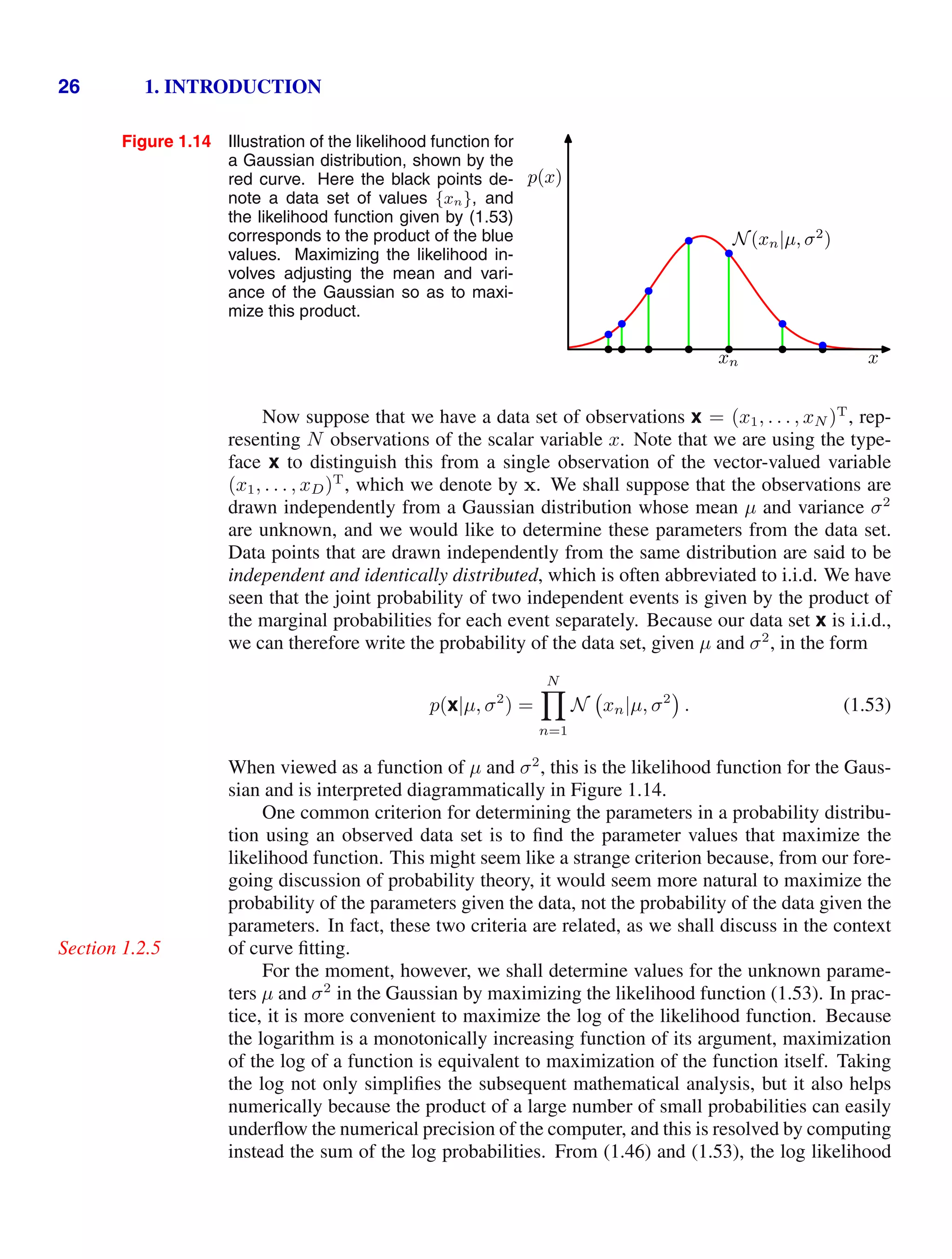
![1.2. Probability Theory 27
function can be written in the form
ln p x|µ, σ2
= −
1
2σ2
N
n=1
(xn − µ)2
−
N
2
ln σ2
−
N
2
ln(2π). (1.54)
Maximizing (1.54) with respect to µ, we obtain the maximum likelihood solution
given by
Exercise 1.11
µML =
1
N
N
n=1
xn (1.55)
which is the sample mean, i.e., the mean of the observed values {xn}. Similarly,
maximizing (1.54) with respect to σ2
, we obtain the maximum likelihood solution
for the variance in the form
σ2
ML =
1
N
N
n=1
(xn − µML)2
(1.56)
which is the sample variance measured with respect to the sample mean µML. Note
that we are performing a joint maximization of (1.54) with respect to µ and σ2
, but
in the case of the Gaussian distribution the solution for µ decouples from that for σ2
so that we can first evaluate (1.55) and then subsequently use this result to evaluate
(1.56).
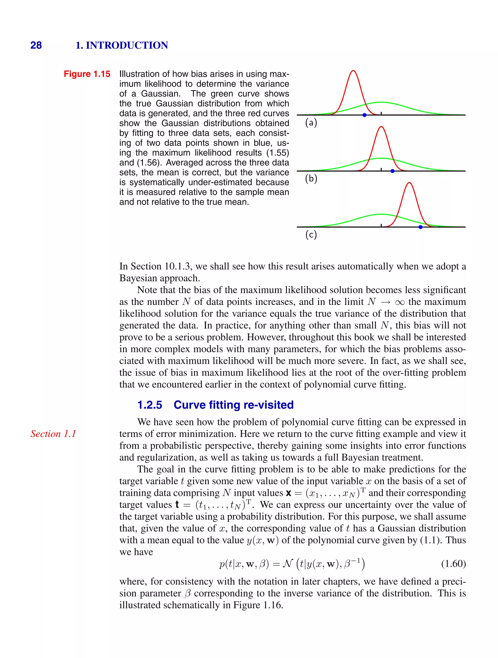
Later in this chapter, and also in subsequent chapters, we shall highlight the sig-
nificant limitations of the maximum likelihood approach. Here we give an indication
of the problem in the context of our solutions for the maximum likelihood param-
eter settings for the univariate Gaussian distribution. In particular, we shall show
that the maximum likelihood approach systematically underestimates the variance
of the distribution. This is an example of a phenomenon called bias and is related
to the problem of over-fitting encountered in the context of polynomial curve fitting.
Section 1.1
We first note that the maximum likelihood solutions µML and σ2
ML are functions of
the data set values x1, . . . , xN . Consider the expectations of these quantities with
respect to the data set values, which themselves come from a Gaussian distribution
with parameters µ and σ2
. It is straightforward to show that
Exercise 1.12
E[µML] = µ (1.57)
E[σ2
ML] =
N − 1
N
σ2
(1.58)
so that on average the maximum likelihood estimate will obtain the correct mean but
will underestimate the true variance by a factor (N − 1)/N. The intuition behind
this result is given by Figure 1.15.
From (1.58) it follows that the following estimate for the variance parameter is
unbiased
σ2
=
N
N − 1
σ2
ML =
1
N − 1
N
n=1
(xn − µML)2
. (1.59)](https://image.slidesharecdn.com/bishop-patternrecognitionandmachinelearning-230316082240-9af1cdaa/75/Bishop-Pattern-Recognition-and-Machine-Learning-pdf-45-2048.jpg)
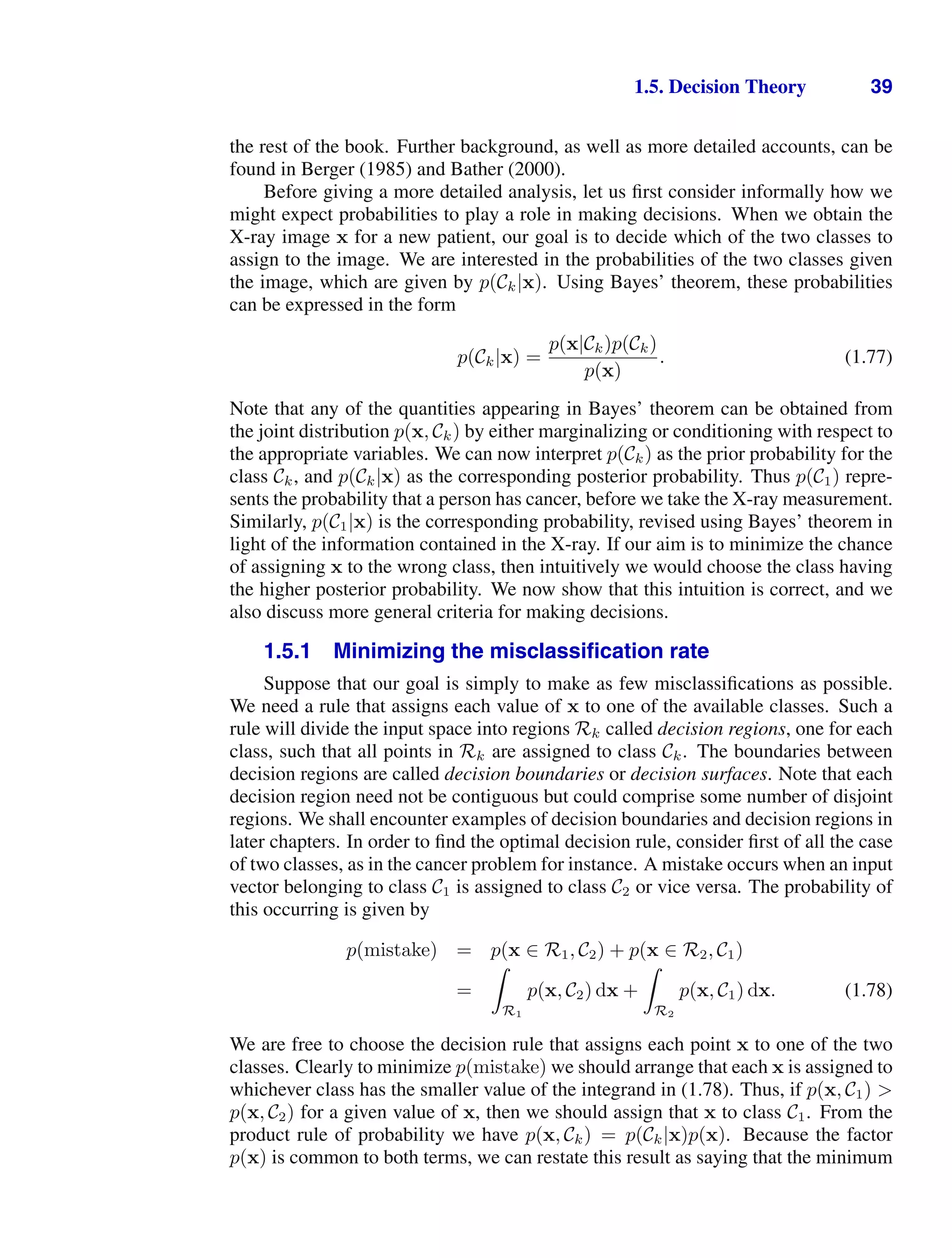
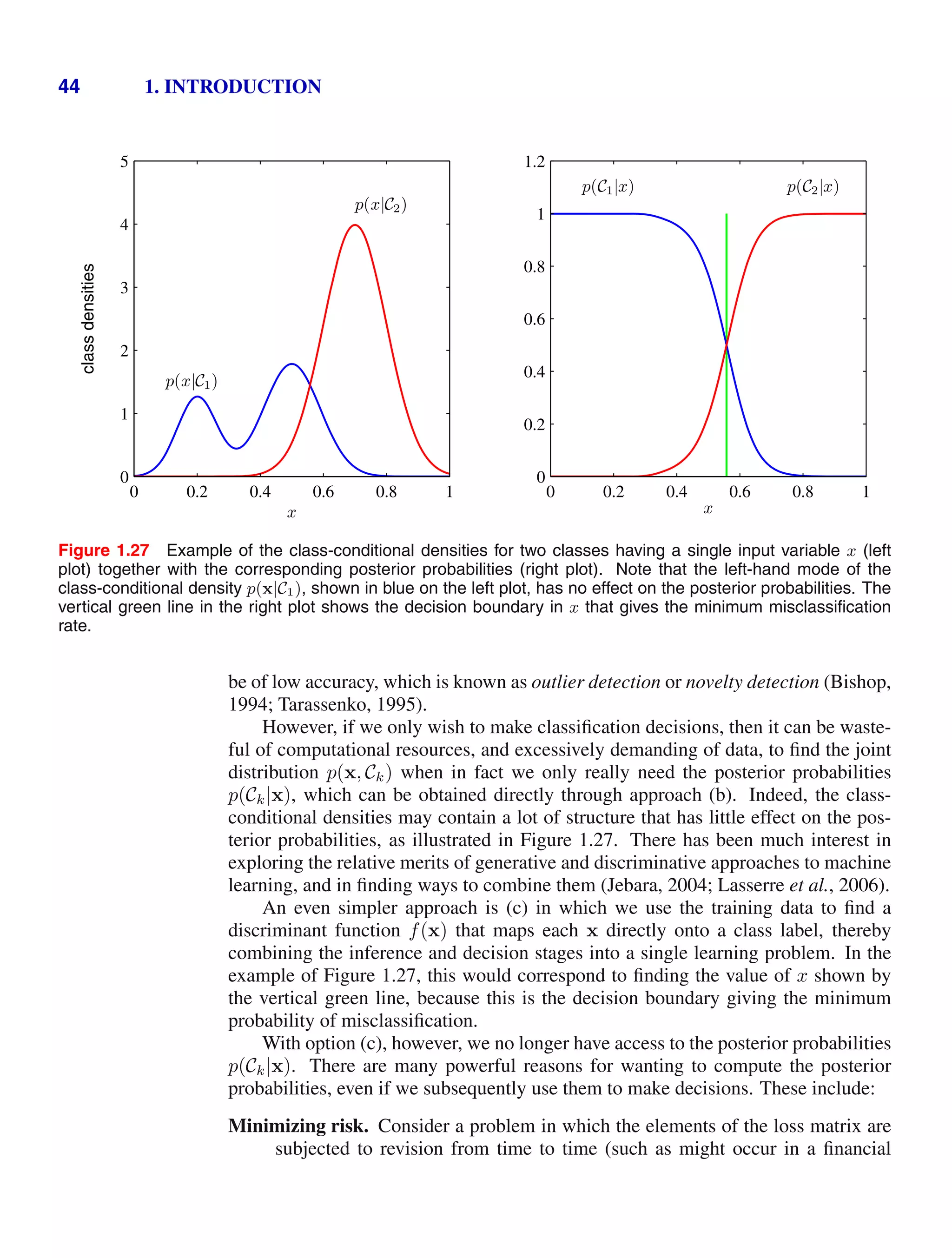
![1.5. Decision Theory 41
Figure 1.25 An example of a loss matrix with ele-
ments Lkj for the cancer treatment problem. The rows
correspond to the true class, whereas the columns cor-
respond to the assignment of class made by our deci-
sion criterion.
cancer normal
cancer 0 1000
normal 1 0
1.5.2 Minimizing the expected loss
For many applications, our objective will be more complex than simply mini-
mizing the number of misclassifications. Let us consider again the medical diagnosis
problem. We note that, if a patient who does not have cancer is incorrectly diagnosed
as having cancer, the consequences may be some patient distress plus the need for
further investigations. Conversely, if a patient with cancer is diagnosed as healthy,
the result may be premature death due to lack of treatment. Thus the consequences
of these two types of mistake can be dramatically different. It would clearly be better
to make fewer mistakes of the second kind, even if this was at the expense of making
more mistakes of the first kind.
We can formalize such issues through the introduction of a loss function, also
called a cost function, which is a single, overall measure of loss incurred in taking
any of the available decisions or actions. Our goal is then to minimize the total loss
incurred. Note that some authors consider instead a utility function, whose value
they aim to maximize. These are equivalent concepts if we take the utility to be
simply the negative of the loss, and throughout this text we shall use the loss function
convention. Suppose that, for a new value of x, the true class is Ck and that we assign
x to class Cj (where j may or may not be equal to k). In so doing, we incur some
level of loss that we denote by Lkj, which we can view as the k, j element of a loss
matrix. For instance, in our cancer example, we might have a loss matrix of the form
shown in Figure 1.25. This particular loss matrix says that there is no loss incurred
if the correct decision is made, there is a loss of 1 if a healthy patient is diagnosed as
having cancer, whereas there is a loss of 1000 if a patient having cancer is diagnosed
as healthy.
The optimal solution is the one which minimizes the loss function. However,
the loss function depends on the true class, which is unknown. For a given input
vector x, our uncertainty in the true class is expressed through the joint probability
distribution p(x, Ck) and so we seek instead to minimize the average loss, where the
average is computed with respect to this distribution, which is given by
E[L] =
k
j
Rj
Lkjp(x, Ck) dx. (1.80)
Each x can be assigned independently to one of the decision regions Rj. Our goal
is to choose the regions Rj in order to minimize the expected loss (1.80), which
implies that for each x we should minimize
k Lkjp(x, Ck). As before, we can use
the product rule p(x, Ck) = p(Ck|x)p(x) to eliminate the common factor of p(x).
Thus the decision rule that minimizes the expected loss is the one that assigns each](https://image.slidesharecdn.com/bishop-patternrecognitionandmachinelearning-230316082240-9af1cdaa/75/Bishop-Pattern-Recognition-and-Machine-Learning-pdf-59-2048.jpg)
![46 1. INTRODUCTION
independent, so that
p(xI, xB|Ck) = p(xI|Ck)p(xB|Ck). (1.84)
This is an example of conditional independence property, because the indepen-
Section 8.2
dence holds when the distribution is conditioned on the class Ck. The posterior
probability, given both the X-ray and blood data, is then given by
p(Ck|xI, xB) ∝ p(xI, xB|Ck)p(Ck)
∝ p(xI|Ck)p(xB|Ck)p(Ck)
∝
p(Ck|xI)p(Ck|xB)
p(Ck)
(1.85)
Thus we need the class prior probabilities p(Ck), which we can easily estimate
from the fractions of data points in each class, and then we need to normalize
the resulting posterior probabilities so they sum to one. The particular condi-
tional independence assumption (1.84) is an example of the naive Bayes model.
Section 8.2.2
Note that the joint marginal distribution p(xI, xB) will typically not factorize
under this model. We shall see in later chapters how to construct models for
combining data that do not require the conditional independence assumption
(1.84).
1.5.5 Loss functions for regression
So far, we have discussed decision theory in the context of classification prob-
lems. We now turn to the case of regression problems, such as the curve fitting
example discussed earlier. The decision stage consists of choosing a specific esti-
Section 1.1
mate y(x) of the value of t for each input x. Suppose that in doing so, we incur a
loss L(t, y(x)). The average, or expected, loss is then given by
E[L] =
L(t, y(x))p(x, t) dx dt. (1.86)
A common choice of loss function in regression problems is the squared loss given
by L(t, y(x)) = {y(x) − t}2
. In this case, the expected loss can be written
E[L] =
{y(x) − t}2
p(x, t) dx dt. (1.87)
Our goal is to choose y(x) so as to minimize E[L]. If we assume a completely
flexible function y(x), we can do this formally using the calculus of variations to
Appendix D
give
δE[L]
δy(x)
= 2
{y(x) − t}p(x, t) dt = 0. (1.88)
Solving for y(x), and using the sum and product rules of probability, we obtain
y(x) =
tp(x, t) dt
p(x)
=
tp(t|x) dt = Et[t|x] (1.89)](https://image.slidesharecdn.com/bishop-patternrecognitionandmachinelearning-230316082240-9af1cdaa/75/Bishop-Pattern-Recognition-and-Machine-Learning-pdf-64-2048.jpg)
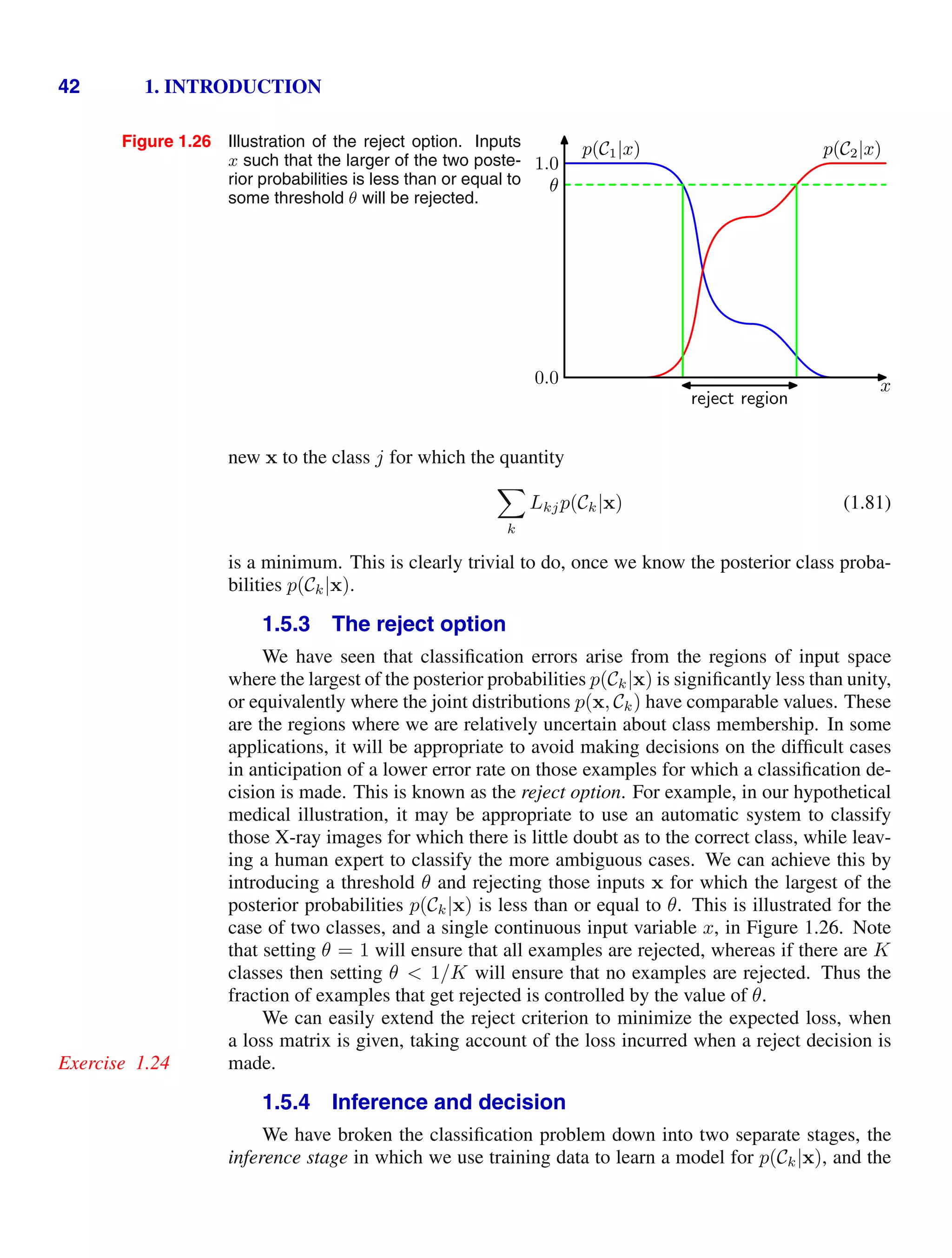
![1.5. Decision Theory 47
Figure 1.28 The regression function y(x),
which minimizes the expected
squared loss, is given by the
mean of the conditional distri-
bution p(t|x).
t
x
x0
y(x0)
y(x)
p(t|x0)
which is the conditional average of t conditioned on x and is known as the regression
function. This result is illustrated in Figure 1.28. It can readily be extended to mul-
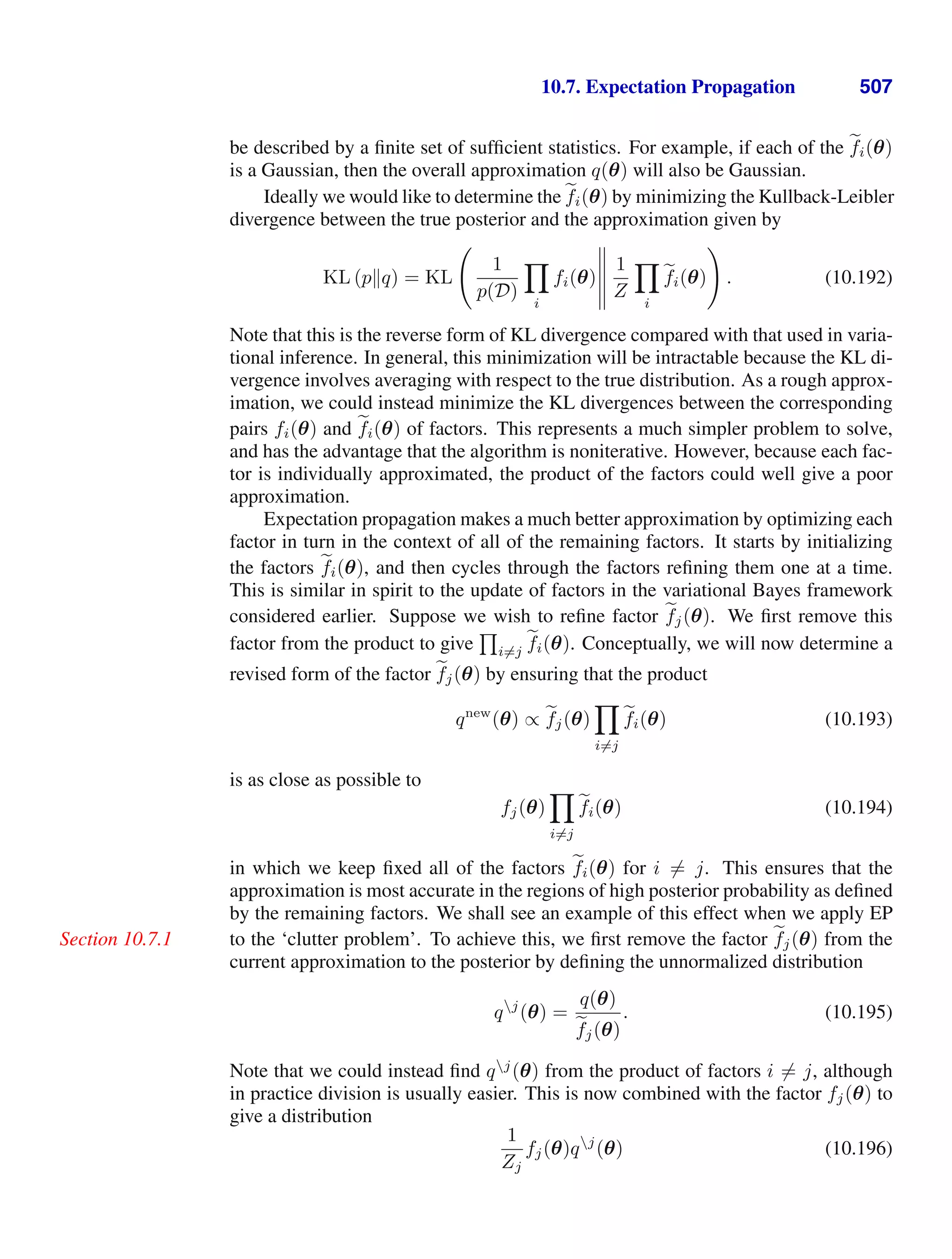
tiple target variables represented by the vector t, in which case the optimal solution
is the conditional average y(x) = Et[t|x].
Exercise 1.25
We can also derive this result in a slightly different way, which will also shed
light on the nature of the regression problem. Armed with the knowledge that the
optimal solution is the conditional expectation, we can expand the square term as
follows
{y(x) − t}2
= {y(x) − E[t|x] + E[t|x] − t}2
= {y(x) − E[t|x]}2
+ 2{y(x) − E[t|x]}{E[t|x] − t} + {E[t|x] − t}2
where, to keep the notation uncluttered, we use E[t|x] to denote Et[t|x]. Substituting
into the loss function and performing the integral over t, we see that the cross-term
vanishes and we obtain an expression for the loss function in the form
E[L] =
{y(x) − E[t|x]}
2
p(x) dx +
{E[t|x] − t}2
p(x) dx. (1.90)
The function y(x) we seek to determine enters only in the first term, which will be
minimized when y(x) is equal to E[t|x], in which case this term will vanish. This
is simply the result that we derived previously and that shows that the optimal least
squares predictor is given by the conditional mean. The second term is the variance
of the distribution of t, averaged over x. It represents the intrinsic variability of
the target data and can be regarded as noise. Because it is independent of y(x), it
represents the irreducible minimum value of the loss function.
As with the classification problem, we can either determine the appropriate prob-
abilities and then use these to make optimal decisions, or we can build models that
make decisions directly. Indeed, we can identify three distinct approaches to solving
regression problems given, in order of decreasing complexity, by:
(a) First solve the inference problem of determining the joint density p(x, t). Then
normalize to find the conditional density p(t|x), and finally marginalize to find
the conditional mean given by (1.89).](https://image.slidesharecdn.com/bishop-patternrecognitionandmachinelearning-230316082240-9af1cdaa/75/Bishop-Pattern-Recognition-and-Machine-Learning-pdf-65-2048.jpg)
![48 1. INTRODUCTION
(b) First solve the inference problem of determining the conditional density p(t|x),
and then subsequently marginalize to find the conditional mean given by (1.89).
(c) Find a regression function y(x) directly from the training data.
The relative merits of these three approaches follow the same lines as for classifica-
tion problems above.
The squared loss is not the only possible choice of loss function for regression.
Indeed, there are situations in which squared loss can lead to very poor results and
where we need to develop more sophisticated approaches. An important example
concerns situations in which the conditional distribution p(t|x) is multimodal, as
often arises in the solution of inverse problems. Here we consider briefly one simple
Section 5.6
generalization of the squared loss, called the Minkowski loss, whose expectation is
given by
E[Lq] =
|y(x) − t|q
p(x, t) dx dt (1.91)
which reduces to the expected squared loss for q = 2. The function |y − t|q
is
plotted against y − t for various values of q in Figure 1.29. The minimum of E[Lq]
is given by the conditional mean for q = 2, the conditional median for q = 1, and
the conditional mode for q → 0.
Exercise 1.27
1.6. Information Theory
In this chapter, we have discussed a variety of concepts from probability theory and
decision theory that will form the foundations for much of the subsequent discussion
in this book. We close this chapter by introducing some additional concepts from
the field of information theory, which will also prove useful in our development of
pattern recognition and machine learning techniques. Again, we shall focus only on
the key concepts, and we refer the reader elsewhere for more detailed discussions
(Viterbi and Omura, 1979; Cover and Thomas, 1991; MacKay, 2003) .
We begin by considering a discrete random variable x and we ask how much
information is received when we observe a specific value for this variable. The
amount of information can be viewed as the ‘degree of surprise’ on learning the
value of x. If we are told that a highly improbable event has just occurred, we will
have received more information than if we were told that some very likely event
has just occurred, and if we knew that the event was certain to happen we would
receive no information. Our measure of information content will therefore depend
on the probability distribution p(x), and we therefore look for a quantity h(x) that
is a monotonic function of the probability p(x) and that expresses the information
content. The form of h(·) can be found by noting that if we have two events x
and y that are unrelated, then the information gain from observing both of them
should be the sum of the information gained from each of them separately, so that
h(x, y) = h(x) + h(y). Two unrelated events will be statistically independent and
so p(x, y) = p(x)p(y). From these two relationships, it is easily shown that h(x)
must be given by the logarithm of p(x) and so we have
Exercise 1.28](https://image.slidesharecdn.com/bishop-patternrecognitionandmachinelearning-230316082240-9af1cdaa/75/Bishop-Pattern-Recognition-and-Machine-Learning-pdf-66-2048.jpg)
![1.6. Information Theory 49
y − t
|y
−
t|
q
q = 0.3
−2 −1 0 1 2
0
1
2
y − t
|y
−
t|
q
q = 1
−2 −1 0 1 2
0
1
2
y − t
|y
−
t|
q
q = 2
−2 −1 0 1 2
0
1
2
y − t
|y
−
t|
q
q = 10
−2 −1 0 1 2
0
1
2
Figure 1.29 Plots of the quantity Lq = |y − t|q
for various values of q.
h(x) = − log2 p(x) (1.92)
where the negative sign ensures that information is positive or zero. Note that low
probability events x correspond to high information content. The choice of basis
for the logarithm is arbitrary, and for the moment we shall adopt the convention
prevalent in information theory of using logarithms to the base of 2. In this case, as
we shall see shortly, the units of h(x) are bits (‘binary digits’).
Now suppose that a sender wishes to transmit the value of a random variable to
a receiver. The average amount of information that they transmit in the process is
obtained by taking the expectation of (1.92) with respect to the distribution p(x) and
is given by
H[x] = −
x
p(x) log2 p(x). (1.93)
This important quantity is called the entropy of the random variable x. Note that
limp→0 p ln p = 0 and so we shall take p(x) ln p(x) = 0 whenever we encounter a
value for x such that p(x) = 0.
So far we have given a rather heuristic motivation for the definition of informa-](https://image.slidesharecdn.com/bishop-patternrecognitionandmachinelearning-230316082240-9af1cdaa/75/Bishop-Pattern-Recognition-and-Machine-Learning-pdf-67-2048.jpg)
![50 1. INTRODUCTION
tion (1.92) and the corresponding entropy (1.93). We now show that these definitions
indeed possess useful properties. Consider a random variable x having 8 possible
states, each of which is equally likely. In order to communicate the value of x to
a receiver, we would need to transmit a message of length 3 bits. Notice that the
entropy of this variable is given by
H[x] = −8 ×
1
8
log2
1
8
= 3 bits.
Now consider an example (Cover and Thomas, 1991) of a variable having 8 pos-
sible states {a, b, c, d, e, f, g, h} for which the respective probabilities are given by
(1
2
, 1
4
, 1
8
, 1
16
, 1
64
, 1
64
, 1
64
, 1
64
). The entropy in this case is given by
H[x] = −
1
2
log2
1
2
−
1
4
log2
1
4
−
1
8
log2
1
8
−
1
16
log2
1
16
−
4
64
log2
1
64
= 2 bits.
We see that the nonuniform distribution has a smaller entropy than the uniform one,
and we shall gain some insight into this shortly when we discuss the interpretation of
entropy in terms of disorder. For the moment, let us consider how we would transmit
the identity of the variable’s state to a receiver. We could do this, as before, using
a 3-bit number. However, we can take advantage of the nonuniform distribution by
using shorter codes for the more probable events, at the expense of longer codes for
the less probable events, in the hope of getting a shorter average code length. This
can be done by representing the states {a, b, c, d, e, f, g, h} using, for instance, the
following set of code strings: 0, 10, 110, 1110, 111100, 111101, 111110, 111111.
The average length of the code that has to be transmitted is then
average code length =
1
2
× 1 +
1
4
× 2 +
1
8
× 3 +
1
16
× 4 + 4 ×
1
64
× 6 = 2 bits
which again is the same as the entropy of the random variable. Note that shorter code
strings cannot be used because it must be possible to disambiguate a concatenation
of such strings into its component parts. For instance, 11001110 decodes uniquely
into the state sequence c, a, d.
This relation between entropy and shortest coding length is a general one. The
noiseless coding theorem (Shannon, 1948) states that the entropy is a lower bound
on the number of bits needed to transmit the state of a random variable.
From now on, we shall switch to the use of natural logarithms in defining en-
tropy, as this will provide a more convenient link with ideas elsewhere in this book.
In this case, the entropy is measured in units of ‘nats’ instead of bits, which differ
simply by a factor of ln 2.
We have introduced the concept of entropy in terms of the average amount of
information needed to specify the state of a random variable. In fact, the concept of
entropy has much earlier origins in physics where it was introduced in the context
of equilibrium thermodynamics and later given a deeper interpretation as a measure
of disorder through developments in statistical mechanics. We can understand this
alternative view of entropy by considering a set of N identical objects that are to be
divided amongst a set of bins, such that there are ni objects in the ith
bin. Consider](https://image.slidesharecdn.com/bishop-patternrecognitionandmachinelearning-230316082240-9af1cdaa/75/Bishop-Pattern-Recognition-and-Machine-Learning-pdf-68-2048.jpg)
![1.6. Information Theory 51
the number of different ways of allocating the objects to the bins. There are N
ways to choose the first object, (N − 1) ways to choose the second object, and
so on, leading to a total of N! ways to allocate all N objects to the bins, where N!
(pronounced ‘factorial N’) denotes the product N ×(N −1)×· · ·×2×1. However,
we don’t wish to distinguish between rearrangements of objects within each bin. In
the ith
bin there are ni! ways of reordering the objects, and so the total number of
ways of allocating the N objects to the bins is given by
W =
N!
i ni!
(1.94)
which is called the multiplicity. The entropy is then defined as the logarithm of the
multiplicity scaled by an appropriate constant
H =
1
N
ln W =
1
N
ln N! −
1
N
i
ln ni!. (1.95)
We now consider the limit N → ∞, in which the fractions ni/N are held fixed, and
apply Stirling’s approximation
ln N! N ln N − N (1.96)
which gives
H = − lim
N→∞
i
ni
N
ln
ni
N
= −
i
pi ln pi (1.97)
where we have used
i ni = N. Here pi = limN→∞(ni/N) is the probability
of an object being assigned to the ith
bin. In physics terminology, the specific ar-
rangements of objects in the bins is called a microstate, and the overall distribution
of occupation numbers, expressed through the ratios ni/N, is called a macrostate.
The multiplicity W is also known as the weight of the macrostate.
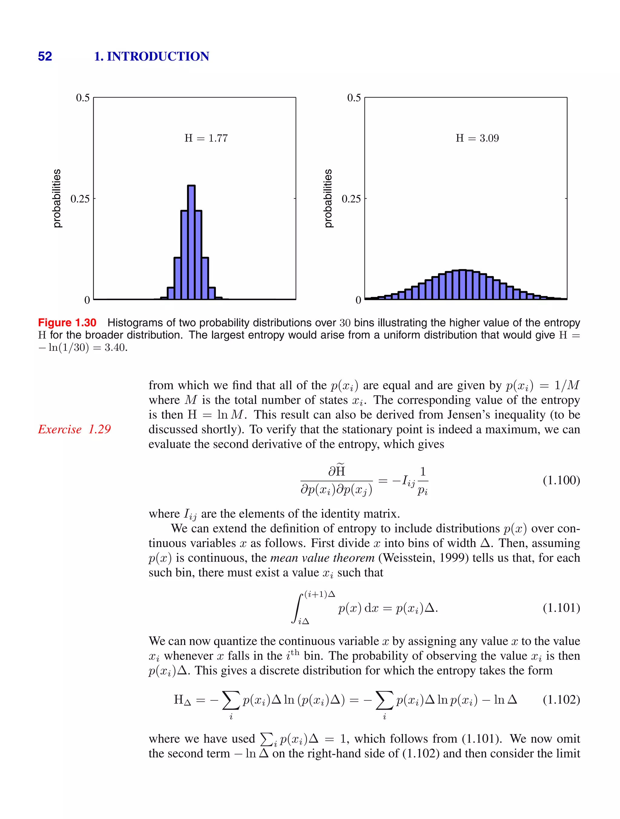
We can interpret the bins as the states xi of a discrete random variable X, where
p(X = xi) = pi. The entropy of the random variable X is then
H[p] = −
i
p(xi) ln p(xi). (1.98)
Distributions p(xi) that are sharply peaked around a few values will have a relatively
low entropy, whereas those that are spread more evenly across many values will
have higher entropy, as illustrated in Figure 1.30. Because 0 pi 1, the entropy
is nonnegative, and it will equal its minimum value of 0 when one of the pi =
1 and all other pj=i = 0. The maximum entropy configuration can be found by
maximizing H using a Lagrange multiplier to enforce the normalization constraint
Appendix E
on the probabilities. Thus we maximize
H = −
i
p(xi) ln p(xi) + λ
i
p(xi) − 1
(1.99)](https://image.slidesharecdn.com/bishop-patternrecognitionandmachinelearning-230316082240-9af1cdaa/75/Bishop-Pattern-Recognition-and-Machine-Learning-pdf-69-2048.jpg)
![1.6. Information Theory 53
∆ → 0. The first term on the right-hand side of (1.102) will approach the integral of
p(x) ln p(x) in this limit so that
lim
∆→0
i
p(xi)∆ ln p(xi)
= −
p(x) ln p(x) dx (1.103)
where the quantity on the right-hand side is called the differential entropy. We see
that the discrete and continuous forms of the entropy differ by a quantity ln ∆, which
diverges in the limit ∆ → 0. This reflects the fact that to specify a continuous
variable very precisely requires a large number of bits. For a density defined over
multiple continuous variables, denoted collectively by the vector x, the differential
entropy is given by
H[x] = −
p(x) ln p(x) dx. (1.104)
In the case of discrete distributions, we saw that the maximum entropy con-
figuration corresponded to an equal distribution of probabilities across the possible
states of the variable. Let us now consider the maximum entropy configuration for
a continuous variable. In order for this maximum to be well defined, it will be nec-
essary to constrain the first and second moments of p(x) as well as preserving the
normalization constraint. We therefore maximize the differential entropy with the
Ludwig Boltzmann
1844–1906
Ludwig Eduard Boltzmann was an
Austrian physicist who created the
field of statistical mechanics. Prior
to Boltzmann, the concept of en-
tropy was already known from
classical thermodynamics where it
quantifies the fact that when we take energy from a
system, not all of that energy is typically available
to do useful work. Boltzmann showed that the ther-
modynamic entropy S, a macroscopic quantity, could
be related to the statistical properties at the micro-
scopic level. This is expressed through the famous
equation S = k ln W in which W represents the
number of possible microstates in a macrostate, and
k 1.38 × 10⁻²³
(in units of Joules per Kelvin) is
known as Boltzmann’s constant. Boltzmann’s ideas
were disputed by many scientists of they day. One dif-
ficulty they saw arose from the second law of thermo-
dynamics, which states that the entropy of a closed
system tends to increase with time. By contrast, at
the microscopic level the classical Newtonian equa-
tions of physics are reversible, and so they found it
difficult to see how the latter could explain the for-
mer. They didn’t fully appreciate Boltzmann’s argu-
ments, which were statistical in nature and which con-
cluded not that entropy could never decrease over
time but simply that with overwhelming probability it
would generally increase. Boltzmann even had a long-
running dispute with the editor of the leading German
physics journal who refused to let him refer to atoms
and molecules as anything other than convenient the-
oretical constructs. The continued attacks on his work
lead to bouts of depression, and eventually he com-
mitted suicide. Shortly after Boltzmann’s death, new
experiments by Perrin on colloidal suspensions veri-
fied his theories and confirmed the value of the Boltz-
mann constant. The equation S = k ln W is carved on
Boltzmann’s tombstone.](https://image.slidesharecdn.com/bishop-patternrecognitionandmachinelearning-230316082240-9af1cdaa/75/Bishop-Pattern-Recognition-and-Machine-Learning-pdf-71-2048.jpg)
![54 1. INTRODUCTION
three constraints
∞
−∞
p(x) dx = 1 (1.105)
∞
−∞
xp(x) dx = µ (1.106)
∞
−∞
(x − µ)2
p(x) dx = σ2
. (1.107)
The constrained maximization can be performed using Lagrange multipliers so that
Appendix E
we maximize the following functional with respect to p(x)
−
∞
−∞
p(x) ln p(x) dx + λ1
∞
−∞
p(x) dx − 1
+λ2
∞
−∞
xp(x) dx − µ
+ λ3
∞
−∞
(x − µ)2
p(x) dx − σ2
.
Using the calculus of variations, we set the derivative of this functional to zero giving
Appendix D
p(x) = exp
−1 + λ1 + λ2x + λ3(x − µ)2
. (1.108)
The Lagrange multipliers can be found by back substitution of this result into the
three constraint equations, leading finally to the result
Exercise 1.34
p(x) =
1
(2πσ2)1/2
exp −
(x − µ)2
2σ2
(1.109)
and so the distribution that maximizes the differential entropy is the Gaussian. Note
that we did not constrain the distribution to be nonnegative when we maximized the
entropy. However, because the resulting distribution is indeed nonnegative, we see
with hindsight that such a constraint is not necessary.
If we evaluate the differential entropy of the Gaussian, we obtain
Exercise 1.35
H[x] =
1
2
1 + ln(2πσ2
)
. (1.110)
Thus we see again that the entropy increases as the distribution becomes broader,
i.e., as σ2
increases. This result also shows that the differential entropy, unlike the
discrete entropy, can be negative, because H(x) 0 in (1.110) for σ2
1/(2πe).
Suppose we have a joint distribution p(x, y) from which we draw pairs of values
of x and y. If a value of x is already known, then the additional information needed
to specify the corresponding value of y is given by − ln p(y|x). Thus the average
additional information needed to specify y can be written as
H[y|x] = −
p(y, x) ln p(y|x) dy dx (1.111)](https://image.slidesharecdn.com/bishop-patternrecognitionandmachinelearning-230316082240-9af1cdaa/75/Bishop-Pattern-Recognition-and-Machine-Learning-pdf-72-2048.jpg)
![1.6. Information Theory 55
which is called the conditional entropy of y given x. It is easily seen, using the
product rule, that the conditional entropy satisfies the relation
Exercise 1.37
H[x, y] = H[y|x] + H[x] (1.112)
where H[x, y] is the differential entropy of p(x, y) and H[x] is the differential en-
tropy of the marginal distribution p(x). Thus the information needed to describe x
and y is given by the sum of the information needed to describe x alone plus the
additional information required to specify y given x.
1.6.1 Relative entropy and mutual information
So far in this section, we have introduced a number of concepts from information
theory, including the key notion of entropy. We now start to relate these ideas to
pattern recognition. Consider some unknown distribution p(x), and suppose that
we have modelled this using an approximating distribution q(x). If we use q(x) to
construct a coding scheme for the purpose of transmitting values of x to a receiver,
then the average additional amount of information (in nats) required to specify the
value of x (assuming we choose an efficient coding scheme) as a result of using q(x)
instead of the true distribution p(x) is given by
KL(pq) = −
p(x) ln q(x) dx −
−
p(x) ln p(x) dx
= −
p(x) ln
q(x)
p(x)
dx. (1.113)
This is known as the relative entropy or Kullback-Leibler divergence, or KL diver-
gence (Kullback and Leibler, 1951), between the distributions p(x) and q(x). Note
that it is not a symmetrical quantity, that is to say KL(pq) ≡ KL(qp).
We now show that the Kullback-Leibler divergence satisfies KL(pq) 0 with
equality if, and only if, p(x) = q(x). To do this we first introduce the concept of
convex functions. A function f(x) is said to be convex if it has the property that
every chord lies on or above the function, as shown in Figure 1.31. Any value of x
in the interval from x = a to x = b can be written in the form λa + (1 − λ)b where
0 λ 1. The corresponding point on the chord is given by λf(a) + (1 − λ)f(b),
Claude Shannon
1916–2001
After graduating from Michigan and
MIT, Shannon joined the ATT Bell
Telephone laboratories in 1941. His
paper ‘A Mathematical Theory of
Communication’ published in the
Bell System Technical Journal in
1948 laid the foundations for modern information the-
ory. This paper introduced the word ‘bit’, and his con-
cept that information could be sent as a stream of 1s
and 0s paved the way for the communications revo-
lution. It is said that von Neumann recommended to
Shannon that he use the term entropy, not only be-
cause of its similarity to the quantity used in physics,
but also because “nobody knows what entropy really
is, so in any discussion you will always have an advan-
tage”.](https://image.slidesharecdn.com/bishop-patternrecognitionandmachinelearning-230316082240-9af1cdaa/75/Bishop-Pattern-Recognition-and-Machine-Learning-pdf-73-2048.jpg)
![56 1. INTRODUCTION
Figure 1.31 A convex function f(x) is one for which ev-
ery chord (shown in blue) lies on or above
the function (shown in red).
x
a b
xλ
chord
xλ
f(x)
and the corresponding value of the function is f (λa + (1 − λ)b). Convexity then
implies
f(λa + (1 − λ)b) λf(a) + (1 − λ)f(b). (1.114)
This is equivalent to the requirement that the second derivative of the function be
everywhere positive. Examples of convex functions are x ln x (for x 0) and x2
. A
Exercise 1.36
function is called strictly convex if the equality is satisfied only for λ = 0 and λ = 1.
If a function has the opposite property, namely that every chord lies on or below the
function, it is called concave, with a corresponding definition for strictly concave. If
a function f(x) is convex, then −f(x) will be concave.
Using the technique of proof by induction, we can show from (1.114) that a
Exercise 1.38
convex function f(x) satisfies
f
M
i=1
λixi
M
i=1
λif(xi) (1.115)
where λi 0 and
i λi = 1, for any set of points {xi}. The result (1.115) is
known as Jensen’s inequality. If we interpret the λi as the probability distribution
over a discrete variable x taking the values {xi}, then (1.115) can be written
f (E[x]) E[f(x)] (1.116)
where E[·] denotes the expectation. For continuous variables, Jensen’s inequality
takes the form
f
xp(x) dx
f(x)p(x) dx. (1.117)
We can apply Jensen’s inequality in the form (1.117) to the Kullback-Leibler
divergence (1.113) to give
KL(pq) = −
p(x) ln
q(x)
p(x)
dx − ln
q(x) dx = 0 (1.118)](https://image.slidesharecdn.com/bishop-patternrecognitionandmachinelearning-230316082240-9af1cdaa/75/Bishop-Pattern-Recognition-and-Machine-Learning-pdf-74-2048.jpg)
![1.6. Information Theory 57
where we have used the fact that − ln x is a convex function, together with the nor-
malization condition
q(x) dx = 1. In fact, − ln x is a strictly convex function,
so the equality will hold if, and only if, q(x) = p(x) for all x. Thus we can in-
terpret the Kullback-Leibler divergence as a measure of the dissimilarity of the two
distributions p(x) and q(x).
We see that there is an intimate relationship between data compression and den-
sity estimation (i.e., the problem of modelling an unknown probability distribution)
because the most efficient compression is achieved when we know the true distri-
bution. If we use a distribution that is different from the true one, then we must
necessarily have a less efficient coding, and on average the additional information
that must be transmitted is (at least) equal to the Kullback-Leibler divergence be-
tween the two distributions.
Suppose that data is being generated from an unknown distribution p(x) that we
wish to model. We can try to approximate this distribution using some parametric
distribution q(x|θ), governed by a set of adjustable parameters θ, for example a
multivariate Gaussian. One way to determine θ is to minimize the Kullback-Leibler
divergence between p(x) and q(x|θ) with respect to θ. We cannot do this directly
because we don’t know p(x). Suppose, however, that we have observed a finite set
of training points xn, for n = 1, . . . , N, drawn from p(x). Then the expectation
with respect to p(x) can be approximated by a finite sum over these points, using
(1.35), so that
KL(pq)
N
n=1
{− ln q(xn|θ) + ln p(xn)} . (1.119)
The second term on the right-hand side of (1.119) is independent of θ, and the first
term is the negative log likelihood function for θ under the distribution q(x|θ) eval-
uated using the training set. Thus we see that minimizing this Kullback-Leibler
divergence is equivalent to maximizing the likelihood function.
Now consider the joint distribution between two sets of variables x and y given
by p(x, y). If the sets of variables are independent, then their joint distribution will
factorize into the product of their marginals p(x, y) = p(x)p(y). If the variables are
not independent, we can gain some idea of whether they are ‘close’ to being indepen-
dent by considering the Kullback-Leibler divergence between the joint distribution
and the product of the marginals, given by
I[x, y] ≡ KL(p(x, y)p(x)p(y))
= −
p(x, y) ln
p(x)p(y)
p(x, y)
dx dy (1.120)
which is called the mutual information between the variables x and y. From the
properties of the Kullback-Leibler divergence, we see that I(x, y) 0 with equal-
ity if, and only if, x and y are independent. Using the sum and product rules of
probability, we see that the mutual information is related to the conditional entropy
through
Exercise 1.41
I[x, y] = H[x] − H[x|y] = H[y] − H[y|x]. (1.121)](https://image.slidesharecdn.com/bishop-patternrecognitionandmachinelearning-230316082240-9af1cdaa/75/Bishop-Pattern-Recognition-and-Machine-Learning-pdf-75-2048.jpg)
![58 1. INTRODUCTION
Thus we can view the mutual information as the reduction in the uncertainty about x
by virtue of being told the value of y (or vice versa). From a Bayesian perspective,
we can view p(x) as the prior distribution for x and p(x|y) as the posterior distribu-
tion after we have observed new data y. The mutual information therefore represents
the reduction in uncertainty about x as a consequence of the new observation y.
Exercises
1.1 () www Consider the sum-of-squares error function given by (1.2) in which
the function y(x, w) is given by the polynomial (1.1). Show that the coefficients
w = {wi} that minimize this error function are given by the solution to the following
set of linear equations
M
j=0
Aijwj = Ti (1.122)
where
Aij =
N
n=1
(xn)i+j
, Ti =
N
n=1
(xn)i
tn. (1.123)
Here a suffix i or j denotes the index of a component, whereas (x)i
denotes x raised
to the power of i.
1.2 () Write down the set of coupled linear equations, analogous to (1.122), satisfied
by the coefficients wi which minimize the regularized sum-of-squares error function
given by (1.4).
1.3 ( ) Suppose that we have three coloured boxes r (red), b (blue), and g (green).
Box r contains 3 apples, 4 oranges, and 3 limes, box b contains 1 apple, 1 orange,
and 0 limes, and box g contains 3 apples, 3 oranges, and 4 limes. If a box is chosen
at random with probabilities p(r) = 0.2, p(b) = 0.2, p(g) = 0.6, and a piece of
fruit is removed from the box (with equal probability of selecting any of the items in
the box), then what is the probability of selecting an apple? If we observe that the
selected fruit is in fact an orange, what is the probability that it came from the green
box?
1.4 ( ) www Consider a probability density px(x) defined over a continuous vari-
able x, and suppose that we make a nonlinear change of variable using x = g(y),
so that the density transforms according to (1.27). By differentiating (1.27), show
that the location
y of the maximum of the density in y is not in general related to the
location
x of the maximum of the density over x by the simple functional relation
x = g(
y) as a consequence of the Jacobian factor. This shows that the maximum
of a probability density (in contrast to a simple function) is dependent on the choice
of variable. Verify that, in the case of a linear transformation, the location of the
maximum transforms in the same way as the variable itself.
1.5 () Using the definition (1.38) show that var[f(x)] satisfies (1.39).](https://image.slidesharecdn.com/bishop-patternrecognitionandmachinelearning-230316082240-9af1cdaa/75/Bishop-Pattern-Recognition-and-Machine-Learning-pdf-76-2048.jpg)
![Exercises 59
1.6 () Show that if two variables x and y are independent, then their covariance is
zero.
1.7 ( ) www In this exercise, we prove the normalization condition (1.48) for the
univariate Gaussian. To do this consider, the integral
I =
∞
−∞
exp
−
1
2σ2
x2
dx (1.124)
which we can evaluate by first writing its square in the form
I2
=
∞
−∞
∞
−∞
exp
−
1
2σ2
x2
−
1
2σ2
y2
dx dy. (1.125)
Now make the transformation from Cartesian coordinates (x, y) to polar coordinates
(r, θ) and then substitute u = r2
. Show that, by performing the integrals over θ and
u, and then taking the square root of both sides, we obtain
I = 2πσ2 1/2
. (1.126)
Finally, use this result to show that the Gaussian distribution N(x|µ, σ2
) is normal-
ized.
1.8 ( ) www By using a change of variables, verify that the univariate Gaussian
distribution given by (1.46) satisfies (1.49). Next, by differentiating both sides of the
normalization condition
∞
−∞
N x|µ, σ2
dx = 1 (1.127)
with respect to σ2
, verify that the Gaussian satisfies (1.50). Finally, show that (1.51)
holds.
1.9 () www Show that the mode (i.e. the maximum) of the Gaussian distribution
(1.46) is given by µ. Similarly, show that the mode of the multivariate Gaussian
(1.52) is given by µ.
1.10 () www Suppose that the two variables x and z are statistically independent.
Show that the mean and variance of their sum satisfies
E[x + z] = E[x] + E[z] (1.128)
var[x + z] = var[x] + var[z]. (1.129)
1.11 () By setting the derivatives of the log likelihood function (1.54) with respect to µ
and σ2
equal to zero, verify the results (1.55) and (1.56).](https://image.slidesharecdn.com/bishop-patternrecognitionandmachinelearning-230316082240-9af1cdaa/75/Bishop-Pattern-Recognition-and-Machine-Learning-pdf-77-2048.jpg)
![60 1. INTRODUCTION
1.12 ( ) www Using the results (1.49) and (1.50), show that
E[xnxm] = µ2
+ Inmσ2
(1.130)
where xn and xm denote data points sampled from a Gaussian distribution with mean
µ and variance σ2
, and Inm satisfies Inm = 1 if n = m and Inm = 0 otherwise.
Hence prove the results (1.57) and (1.58).
1.13 () Suppose that the variance of a Gaussian is estimated using the result (1.56) but
with the maximum likelihood estimate µML replaced with the true value µ of the
mean. Show that this estimator has the property that its expectation is given by the
true variance σ2
.
1.14 ( ) Show that an arbitrary square matrix with elements wij can be written in
the form wij = wS
ij + wA
ij where wS
ij and wA
ij are symmetric and anti-symmetric
matrices, respectively, satisfying wS
ij = wS
ji and wA
ij = −wA
ji for all i and j. Now
consider the second order term in a higher order polynomial in D dimensions, given
by
D
i=1
D
j=1
wijxixj. (1.131)
Show that
D
i=1
D
j=1
wijxixj =
D
i=1
D
j=1
wS
ijxixj (1.132)
so that the contribution from the anti-symmetric matrix vanishes. We therefore see
that, without loss of generality, the matrix of coefficients wij can be chosen to be
symmetric, and so not all of the D2
elements of this matrix can be chosen indepen-
dently. Show that the number of independent parameters in the matrix wS
ij is given
by D(D + 1)/2.
1.15 ( ) www In this exercise and the next, we explore how the number of indepen-
dent parameters in a polynomial grows with the order M of the polynomial and with
the dimensionality D of the input space. We start by writing down the Mth
order
term for a polynomial in D dimensions in the form
D
i1=1
D
i2=1
· · ·
D
iM =1
wi1i2···iM
xi1
xi2
· · · xiM
. (1.133)
The coefficients wi1i2···iM
comprise DM
elements, but the number of independent
parameters is significantly fewer due to the many interchange symmetries of the
factor xi1
xi2
· · · xiM
. Begin by showing that the redundancy in the coefficients can
be removed by rewriting this Mth
order term in the form
D
i1=1
i1
i2=1
· · ·
iM−1
iM =1
wi1i2···iM
xi1
xi2
· · · xiM
. (1.134)](https://image.slidesharecdn.com/bishop-patternrecognitionandmachinelearning-230316082240-9af1cdaa/75/Bishop-Pattern-Recognition-and-Machine-Learning-pdf-78-2048.jpg)
![64 1. INTRODUCTION
1.24 ( ) www Consider a classification problem in which the loss incurred when
an input vector from class Ck is classified as belonging to class Cj is given by the
loss matrix Lkj, and for which the loss incurred in selecting the reject option is λ.
Find the decision criterion that will give the minimum expected loss. Verify that this
reduces to the reject criterion discussed in Section 1.5.3 when the loss matrix is given
by Lkj = 1 − Ikj. What is the relationship between λ and the rejection threshold θ?
1.25 () www Consider the generalization of the squared loss function (1.87) for a
single target variable t to the case of multiple target variables described by the vector
t given by
E[L(t, y(x))] =
y(x) − t2
p(x, t) dx dt. (1.151)
Using the calculus of variations, show that the function y(x) for which this expected
loss is minimized is given by y(x) = Et[t|x]. Show that this result reduces to (1.89)
for the case of a single target variable t.
1.26 () By expansion of the square in (1.151), derive a result analogous to (1.90) and
hence show that the function y(x) that minimizes the expected squared loss for the
case of a vector t of target variables is again given by the conditional expectation of
t.
1.27 ( ) www Consider the expected loss for regression problems under the Lq loss
function given by (1.91). Write down the condition that y(x) must satisfy in order
to minimize E[Lq]. Show that, for q = 1, this solution represents the conditional
median, i.e., the function y(x) such that the probability mass for t y(x) is the
same as for t y(x). Also show that the minimum expected Lq loss for q → 0 is
given by the conditional mode, i.e., by the function y(x) equal to the value of t that
maximizes p(t|x) for each x.
1.28 () In Section 1.6, we introduced the idea of entropy h(x) as the information gained
on observing the value of a random variable x having distribution p(x). We saw
that, for independent variables x and y for which p(x, y) = p(x)p(y), the entropy
functions are additive, so that h(x, y) = h(x) + h(y). In this exercise, we derive the
relation between h and p in the form of a function h(p). First show that h(p2
) =
2h(p), and hence by induction that h(pn
) = nh(p) where n is a positive integer.
Hence show that h(pn/m
) = (n/m)h(p) where m is also a positive integer. This
implies that h(px
) = xh(p) where x is a positive rational number, and hence by
continuity when it is a positive real number. Finally, show that this implies h(p)
must take the form h(p) ∝ ln p.
1.29 () www Consider an M-state discrete random variable x, and use Jensen’s in-
equality in the form (1.115) to show that the entropy of its distribution p(x) satisfies
H[x] ln M.
1.30 ( ) Evaluate the Kullback-Leibler divergence (1.113) between two Gaussians
p(x) = N(x|µ, σ2
) and q(x) = N(x|m, s2
).](https://image.slidesharecdn.com/bishop-patternrecognitionandmachinelearning-230316082240-9af1cdaa/75/Bishop-Pattern-Recognition-and-Machine-Learning-pdf-82-2048.jpg)
![Exercises 65
Table 1.3 The joint distribution p(x, y) for two binary variables
x and y used in Exercise 1.39.
y
0 1
x
0 1/3 1/3
1 0 1/3
1.31 ( ) www Consider two variables x and y having joint distribution p(x, y). Show
that the differential entropy of this pair of variables satisfies
H[x, y] H[x] + H[y] (1.152)
with equality if, and only if, x and y are statistically independent.
1.32 () Consider a vector x of continuous variables with distribution p(x) and corre-
sponding entropy H[x]. Suppose that we make a nonsingular linear transformation
of x to obtain a new variable y = Ax. Show that the corresponding entropy is given
by H[y] = H[x] + ln |A| where |A| denotes the determinant of A.
1.33 ( ) Suppose that the conditional entropy H[y|x] between two discrete random
variables x and y is zero. Show that, for all values of x such that p(x) 0, the
variable y must be a function of x, in other words for each x there is only one value
of y such that p(y|x) = 0.
1.34 ( ) www Use the calculus of variations to show that the stationary point of the
functional (1.108) is given by (1.108). Then use the constraints (1.105), (1.106),
and (1.107) to eliminate the Lagrange multipliers and hence show that the maximum
entropy solution is given by the Gaussian (1.109).
1.35 () www Use the results (1.106) and (1.107) to show that the entropy of the
univariate Gaussian (1.109) is given by (1.110).
1.36 () A strictly convex function is defined as one for which every chord lies above
the function. Show that this is equivalent to the condition that the second derivative
of the function be positive.
1.37 () Using the definition (1.111) together with the product rule of probability, prove
the result (1.112).
1.38 ( ) www Using proof by induction, show that the inequality (1.114) for convex
functions implies the result (1.115).
1.39 ( ) Consider two binary variables x and y having the joint distribution given in
Table 1.3.
Evaluate the following quantities
(a) H[x] (c) H[y|x] (e) H[x, y]
(b) H[y] (d) H[x|y] (f) I[x, y].
Draw a diagram to show the relationship between these various quantities.](https://image.slidesharecdn.com/bishop-patternrecognitionandmachinelearning-230316082240-9af1cdaa/75/Bishop-Pattern-Recognition-and-Machine-Learning-pdf-83-2048.jpg)

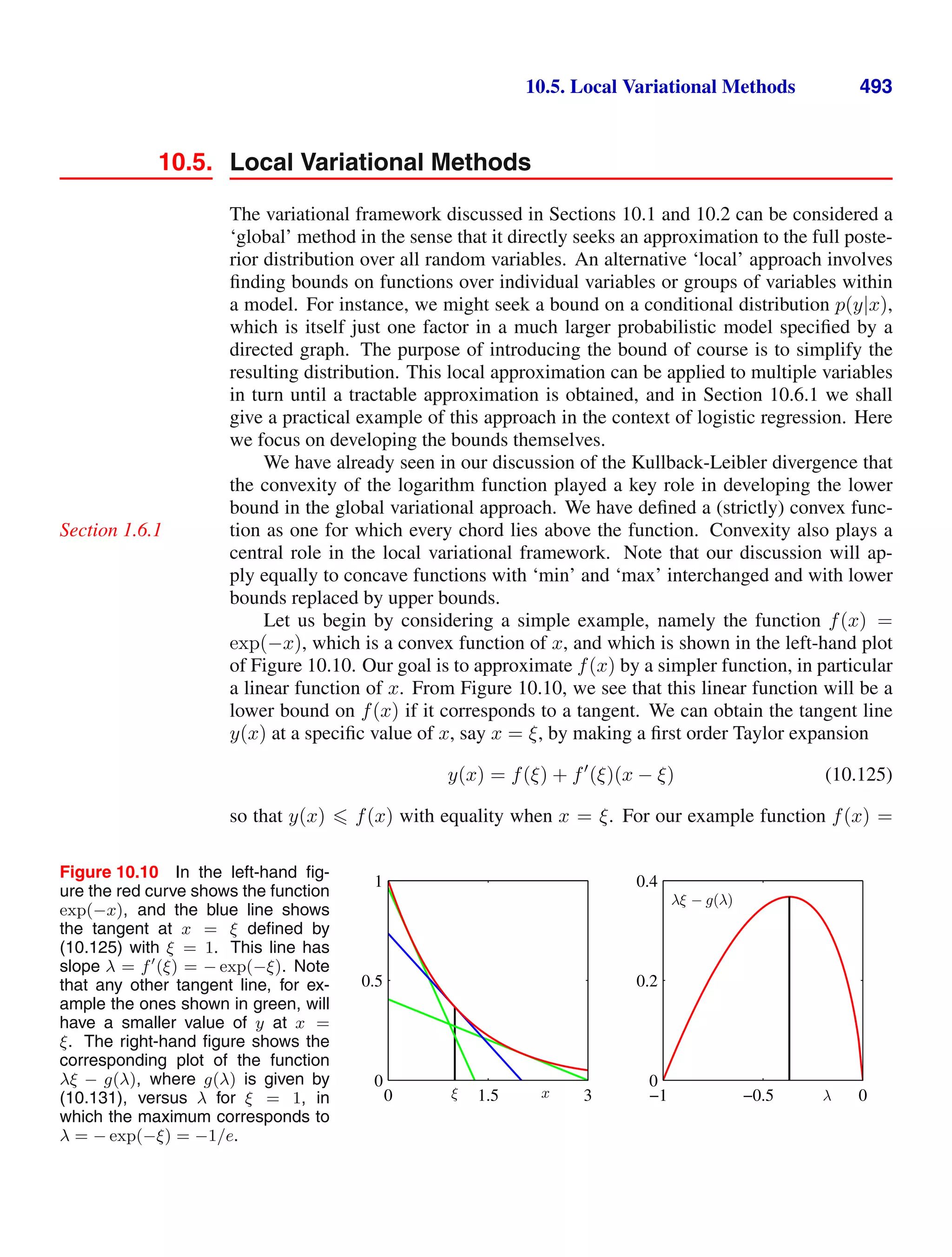
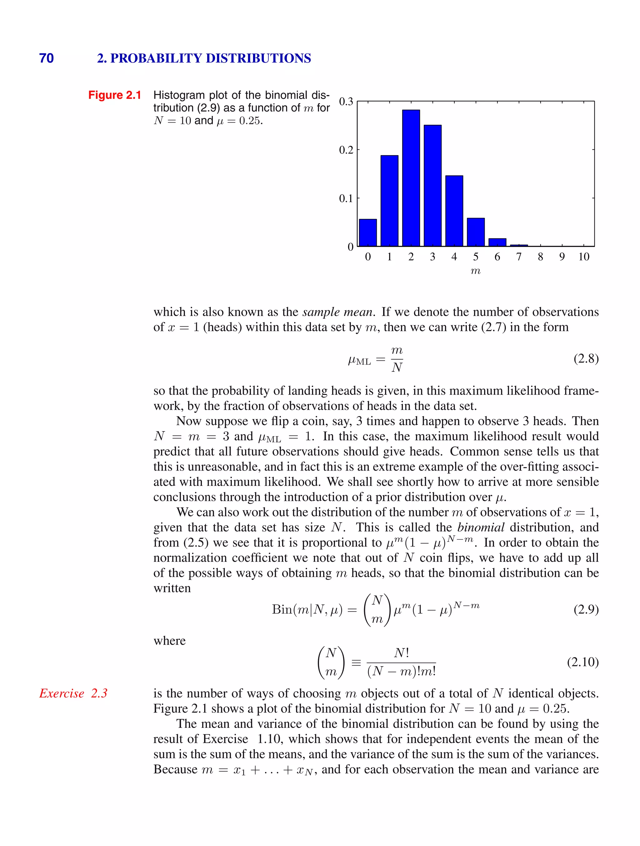
![2.1. Binary Variables 69
where 0 µ 1, from which it follows that p(x = 0|µ) = 1 − µ. The probability
distribution over x can therefore be written in the form
Bern(x|µ) = µx
(1 − µ)1−x
(2.2)
which is known as the Bernoulli distribution. It is easily verified that this distribution
Exercise 2.1
is normalized and that it has mean and variance given by
E[x] = µ (2.3)
var[x] = µ(1 − µ). (2.4)
Now suppose we have a data set D = {x1, . . . , xN } of observed values of x.
We can construct the likelihood function, which is a function of µ, on the assumption
that the observations are drawn independently from p(x|µ), so that
p(D|µ) =
N
n=1
p(xn|µ) =
N
n=1
µxn
(1 − µ)1−xn
. (2.5)
In a frequentist setting, we can estimate a value for µ by maximizing the likelihood
function, or equivalently by maximizing the logarithm of the likelihood. In the case
of the Bernoulli distribution, the log likelihood function is given by
ln p(D|µ) =
N
n=1
ln p(xn|µ) =
N
n=1
{xn ln µ + (1 − xn) ln(1 − µ)} . (2.6)
At this point, it is worth noting that the log likelihood function depends on the N
observations xn only through their sum
n xn. This sum provides an example of a
sufficient statistic for the data under this distribution, and we shall study the impor-
tant role of sufficient statistics in some detail. If we set the derivative of ln p(D|µ)
Section 2.4
with respect to µ equal to zero, we obtain the maximum likelihood estimator
µML =
1
N
N
n=1
xn (2.7)
Jacob Bernoulli
1654–1705
Jacob Bernoulli, also known as
Jacques or James Bernoulli, was a
Swiss mathematician and was the
first of many in the Bernoulli family
to pursue a career in science and
mathematics. Although compelled
to study philosophy and theology against his will by
his parents, he travelled extensively after graduating
in order to meet with many of the leading scientists of
his time, including Boyle and Hooke in England. When
he returned to Switzerland, he taught mechanics and
became Professor of Mathematics at Basel in 1687.
Unfortunately, rivalry between Jacob and his younger
brother Johann turned an initially productive collabora-
tion into a bitter and public dispute. Jacob’s most sig-
nificant contributions to mathematics appeared in The
Art of Conjecture published in 1713, eight years after
his death, which deals with topics in probability the-
ory including what has become known as the Bernoulli
distribution.](https://image.slidesharecdn.com/bishop-patternrecognitionandmachinelearning-230316082240-9af1cdaa/75/Bishop-Pattern-Recognition-and-Machine-Learning-pdf-87-2048.jpg)
![2.1. Binary Variables 71
given by (2.3) and (2.4), respectively, we have
E[m] ≡
N
m=0
mBin(m|N, µ) = Nµ (2.11)
var[m] ≡
N
m=0
(m − E[m])
2
Bin(m|N, µ) = Nµ(1 − µ). (2.12)
These results can also be proved directly using calculus.
Exercise 2.4
2.1.1 The beta distribution
We have seen in (2.8) that the maximum likelihood setting for the parameter µ
in the Bernoulli distribution, and hence in the binomial distribution, is given by the
fraction of the observations in the data set having x = 1. As we have already noted,
this can give severely over-fitted results for small data sets. In order to develop a
Bayesian treatment for this problem, we need to introduce a prior distribution p(µ)
over the parameter µ. Here we consider a form of prior distribution that has a simple
interpretation as well as some useful analytical properties. To motivate this prior,
we note that the likelihood function takes the form of the product of factors of the
form µx
(1 − µ)1−x
. If we choose a prior to be proportional to powers of µ and
(1 − µ), then the posterior distribution, which is proportional to the product of the
prior and the likelihood function, will have the same functional form as the prior.
This property is called conjugacy and we will see several examples of it later in this
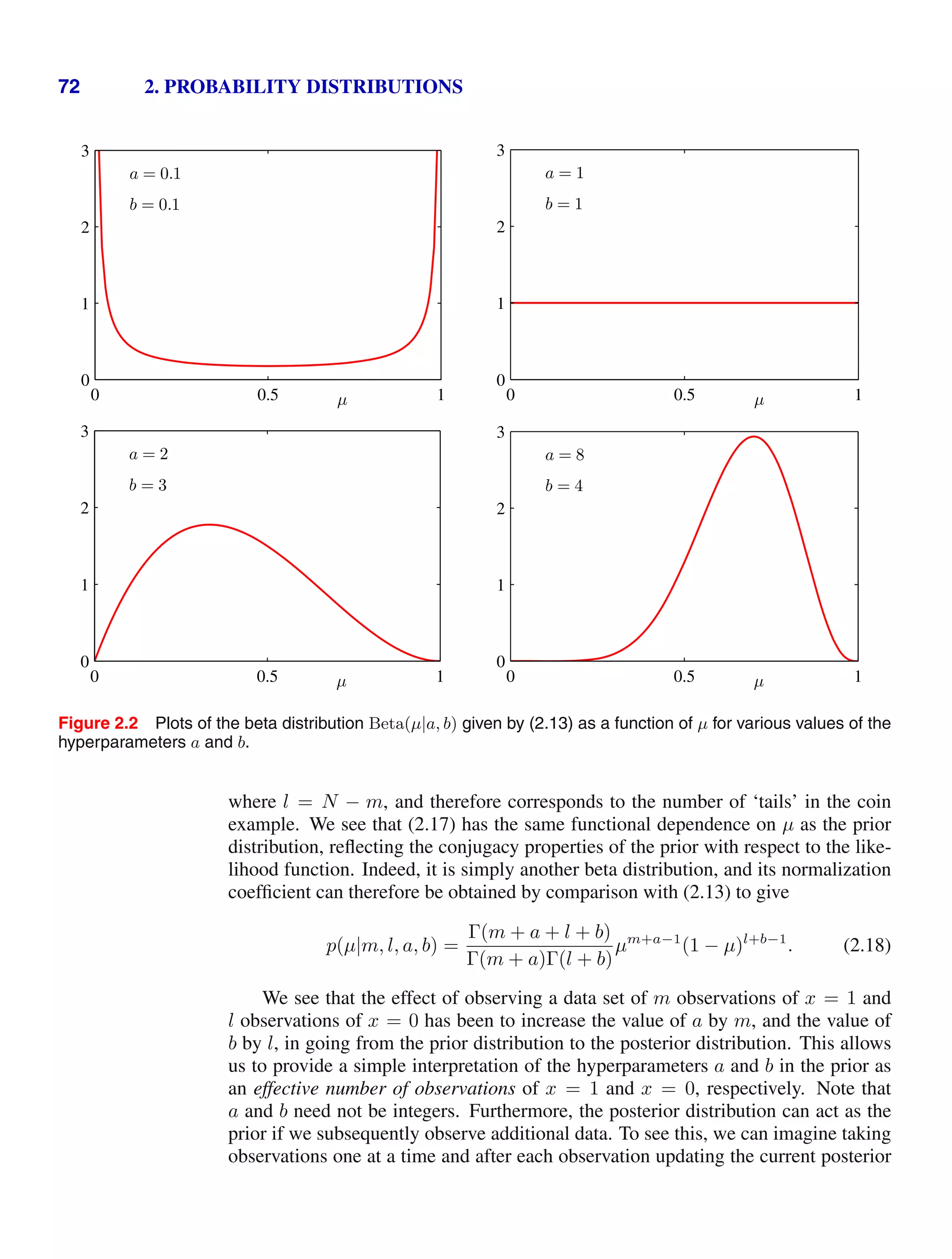
chapter. We therefore choose a prior, called the beta distribution, given by
Beta(µ|a, b) =
Γ(a + b)
Γ(a)Γ(b)
µa−1
(1 − µ)b−1
(2.13)
where Γ(x) is the gamma function defined by (1.141), and the coefficient in (2.13)
ensures that the beta distribution is normalized, so that
Exercise 2.5
1
0
Beta(µ|a, b) dµ = 1. (2.14)
The mean and variance of the beta distribution are given by
Exercise 2.6
E[µ] =
a
a + b
(2.15)
var[µ] =
ab
(a + b)2(a + b + 1)
. (2.16)
The parameters a and b are often called hyperparameters because they control the
distribution of the parameter µ. Figure 2.2 shows plots of the beta distribution for
various values of the hyperparameters.
The posterior distribution of µ is now obtained by multiplying the beta prior
(2.13) by the binomial likelihood function (2.9) and normalizing. Keeping only the
factors that depend on µ, we see that this posterior distribution has the form
p(µ|m, l, a, b) ∝ µm+a−1
(1 − µ)l+b−1
(2.17)](https://image.slidesharecdn.com/bishop-patternrecognitionandmachinelearning-230316082240-9af1cdaa/75/Bishop-Pattern-Recognition-and-Machine-Learning-pdf-89-2048.jpg)
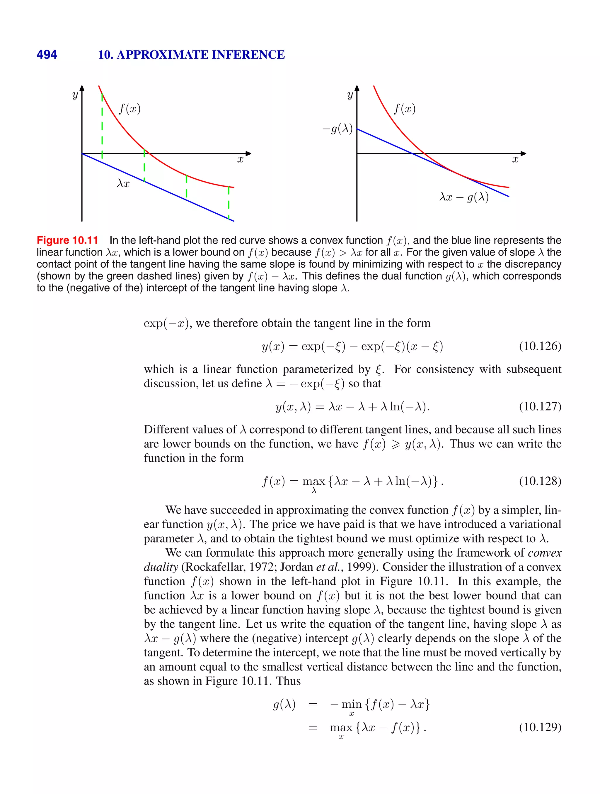
![2.1. Binary Variables 73
µ
prior
0 0.5 1
0
1
2
µ
likelihood function
0 0.5 1
0
1
2
µ
posterior
0 0.5 1
0
1
2
Figure 2.3 Illustration of one step of sequential Bayesian inference. The prior is given by a beta distribution
with parameters a = 2, b = 2, and the likelihood function, given by (2.9) with N = m = 1, corresponds to a
single observation of x = 1, so that the posterior is given by a beta distribution with parameters a = 3, b = 2.
distribution by multiplying by the likelihood function for the new observation and
then normalizing to obtain the new, revised posterior distribution. At each stage, the
posterior is a beta distribution with some total number of (prior and actual) observed
values for x = 1 and x = 0 given by the parameters a and b. Incorporation of an
additional observation of x = 1 simply corresponds to incrementing the value of a
by 1, whereas for an observation of x = 0 we increment b by 1. Figure 2.3 illustrates
one step in this process.
We see that this sequential approach to learning arises naturally when we adopt
a Bayesian viewpoint. It is independent of the choice of prior and of the likelihood
function and depends only on the assumption of i.i.d. data. Sequential methods make
use of observations one at a time, or in small batches, and then discard them before
the next observations are used. They can be used, for example, in real-time learning
scenarios where a steady stream of data is arriving, and predictions must be made
before all of the data is seen. Because they do not require the whole data set to be
stored or loaded into memory, sequential methods are also useful for large data sets.
Maximum likelihood methods can also be cast into a sequential framework.
Section 2.3.5
If our goal is to predict, as best we can, the outcome of the next trial, then we
must evaluate the predictive distribution of x, given the observed data set D. From
the sum and product rules of probability, this takes the form
p(x = 1|D) =
1
0
p(x = 1|µ)p(µ|D) dµ =
1
0
µp(µ|D) dµ = E[µ|D]. (2.19)
Using the result (2.18) for the posterior distribution p(µ|D), together with the result
(2.15) for the mean of the beta distribution, we obtain
p(x = 1|D) =
m + a
m + a + l + b
(2.20)
which has a simple interpretation as the total fraction of observations (both real ob-
servations and fictitious prior observations) that correspond to x = 1. Note that in
the limit of an infinitely large data set m, l → ∞ the result (2.20) reduces to the
maximum likelihood result (2.8). As we shall see, it is a very general property that
the Bayesian and maximum likelihood results will agree in the limit of an infinitely](https://image.slidesharecdn.com/bishop-patternrecognitionandmachinelearning-230316082240-9af1cdaa/75/Bishop-Pattern-Recognition-and-Machine-Learning-pdf-91-2048.jpg)
![74 2. PROBABILITY DISTRIBUTIONS
large data set. For a finite data set, the posterior mean for µ always lies between the
prior mean and the maximum likelihood estimate for µ corresponding to the relative
frequencies of events given by (2.7).
Exercise 2.7
From Figure 2.2, we see that as the number of observations increases, so the
posterior distribution becomes more sharply peaked. This can also be seen from
the result (2.16) for the variance of the beta distribution, in which we see that the
variance goes to zero for a → ∞ or b → ∞. In fact, we might wonder whether it is
a general property of Bayesian learning that, as we observe more and more data, the
uncertainty represented by the posterior distribution will steadily decrease.
To address this, we can take a frequentist view of Bayesian learning and show
that, on average, such a property does indeed hold. Consider a general Bayesian
inference problem for a parameter θ for which we have observed a data set D, de-
scribed by the joint distribution p(θ, D). The following result
Exercise 2.8
Eθ[θ] = ED [Eθ[θ|D]] (2.21)
where
Eθ[θ] ≡
p(θ)θ dθ (2.22)
ED[Eθ[θ|D]] ≡
θp(θ|D) dθ p(D) dD (2.23)
says that the posterior mean of θ, averaged over the distribution generating the data,
is equal to the prior mean of θ. Similarly, we can show that
varθ[θ] = ED [varθ[θ|D]] + varD [Eθ[θ|D]] . (2.24)
The term on the left-hand side of (2.24) is the prior variance of θ. On the right-
hand side, the first term is the average posterior variance of θ, and the second term
measures the variance in the posterior mean of θ. Because this variance is a positive
quantity, this result shows that, on average, the posterior variance of θ is smaller than
the prior variance. The reduction in variance is greater if the variance in the posterior
mean is greater. Note, however, that this result only holds on average, and that for a
particular observed data set it is possible for the posterior variance to be larger than
the prior variance.
2.2. Multinomial Variables
Binary variables can be used to describe quantities that can take one of two possible
values. Often, however, we encounter discrete variables that can take on one of K
possible mutually exclusive states. Although there are various alternative ways to
express such variables, we shall see shortly that a particularly convenient represen-
tation is the 1-of-K scheme in which the variable is represented by a K-dimensional
vector x in which one of the elements xk equals 1, and all remaining elements equal](https://image.slidesharecdn.com/bishop-patternrecognitionandmachinelearning-230316082240-9af1cdaa/75/Bishop-Pattern-Recognition-and-Machine-Learning-pdf-92-2048.jpg)
![2.2. Multinomial Variables 75
0. So, for instance if we have a variable that can take K = 6 states and a particular
observation of the variable happens to correspond to the state where x3 = 1, then x
will be represented by
x = (0, 0, 1, 0, 0, 0)T
. (2.25)
Note that such vectors satisfy
K
k=1 xk = 1. If we denote the probability of xk = 1
by the parameter µk, then the distribution of x is given
p(x|µ) =
K
k=1
µxk
k (2.26)
where µ = (µ1, . . . , µK)T
, and the parameters µk are constrained to satisfy µk 0
and
k µk = 1, because they represent probabilities. The distribution (2.26) can be
regarded as a generalization of the Bernoulli distribution to more than two outcomes.
It is easily seen that the distribution is normalized
x
p(x|µ) =
K
k=1
µk = 1 (2.27)
and that
E[x|µ] =
x
p(x|µ)x = (µ1, . . . , µM )T
= µ. (2.28)
Now consider a data set D of N independent observations x1, . . . , xN . The
corresponding likelihood function takes the form
p(D|µ) =
N
n=1
K
k=1
µxnk
k =
K
k=1
µ
(
P
n xnk)
k =
K
k=1
µmk
k . (2.29)
We see that the likelihood function depends on the N data points only through the
K quantities
mk =
n
xnk (2.30)
which represent the number of observations of xk = 1. These are called the sufficient
statistics for this distribution.
Section 2.4
In order to find the maximum likelihood solution for µ, we need to maximize
ln p(D|µ) with respect to µk taking account of the constraint that the µk must sum
to one. This can be achieved using a Lagrange multiplier λ and maximizing
Appendix E
K
k=1
mk ln µk + λ
K
k=1
µk − 1
. (2.31)
Setting the derivative of (2.31) with respect to µk to zero, we obtain
µk = −mk/λ. (2.32)](https://image.slidesharecdn.com/bishop-patternrecognitionandmachinelearning-230316082240-9af1cdaa/75/Bishop-Pattern-Recognition-and-Machine-Learning-pdf-93-2048.jpg)
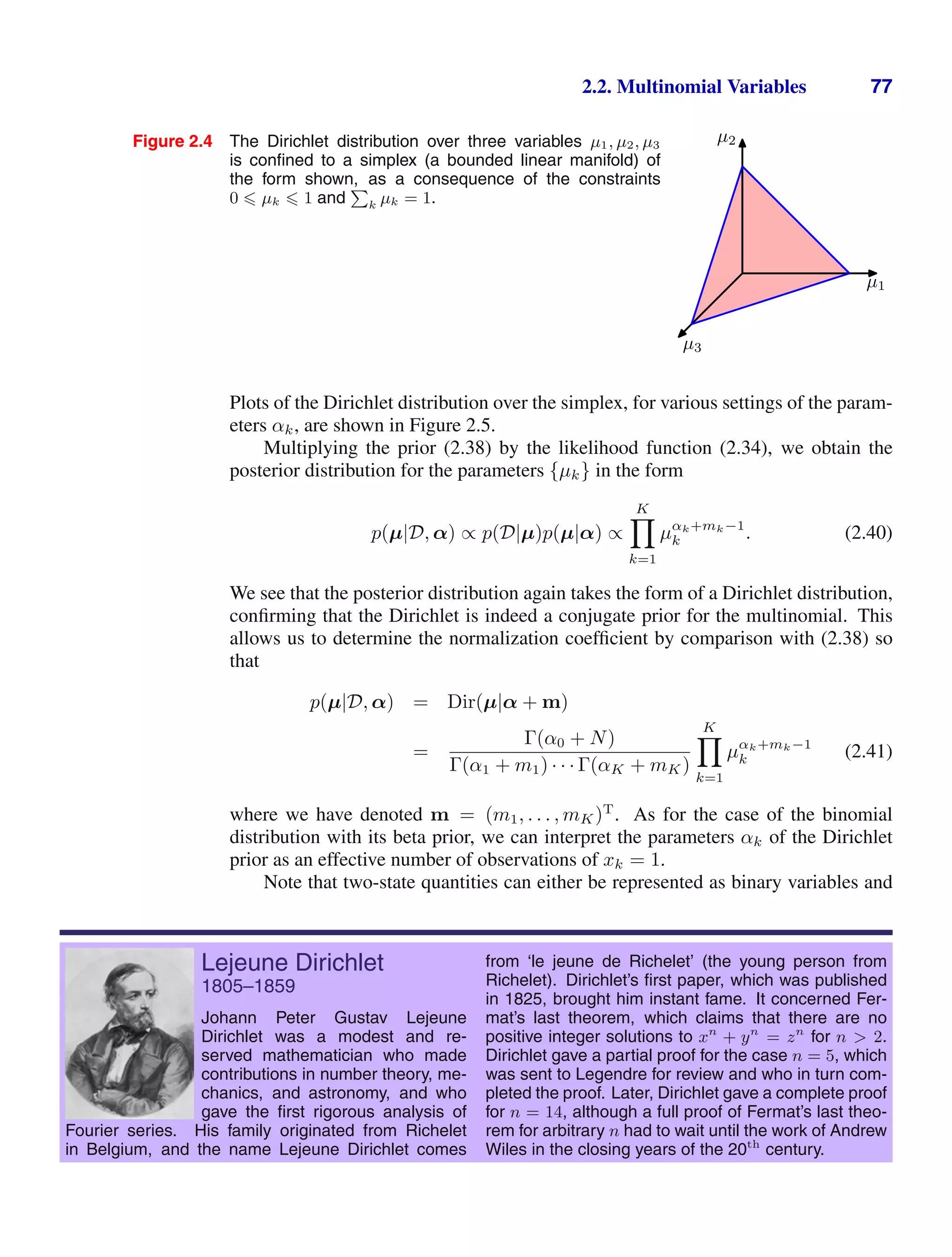
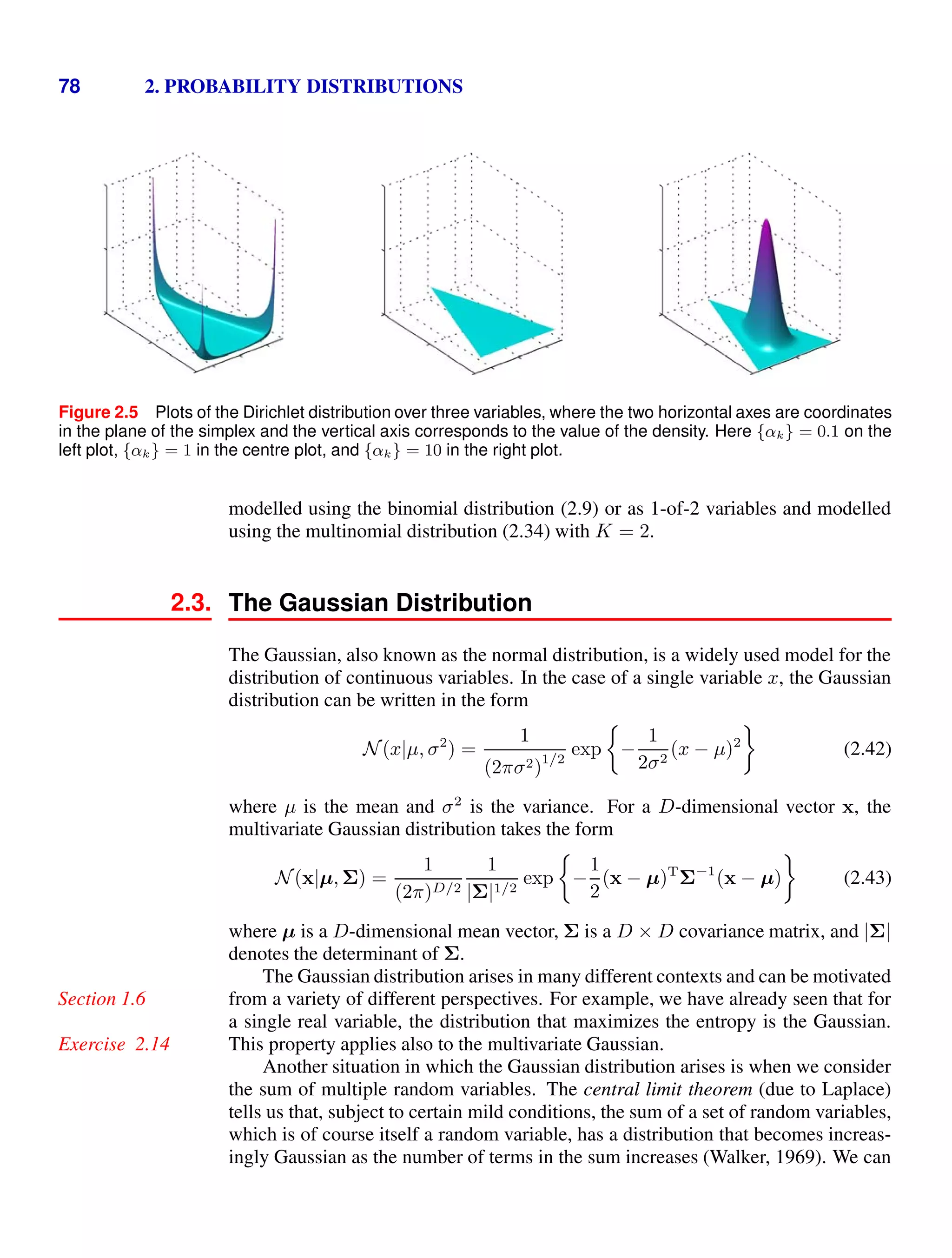
![2.3. The Gaussian Distribution 79
N = 1
0 0.5 1
0
1
2
3
N = 2
0 0.5 1
0
1
2
3
N = 10
0 0.5 1
0
1
2
3
Figure 2.6 Histogram plots of the mean of N uniformly distributed numbers for various values of N. We
observe that as N increases, the distribution tends towards a Gaussian.
illustrate this by considering N variables x1, . . . , xN each of which has a uniform
distribution over the interval [0, 1] and then considering the distribution of the mean
(x1 + · · · + xN )/N. For large N, this distribution tends to a Gaussian, as illustrated
in Figure 2.6. In practice, the convergence to a Gaussian as N increases can be
very rapid. One consequence of this result is that the binomial distribution (2.9),
which is a distribution over m defined by the sum of N observations of the random
binary variable x, will tend to a Gaussian as N → ∞ (see Figure 2.1 for the case of
N = 10).
The Gaussian distribution has many important analytical properties, and we shall
consider several of these in detail. As a result, this section will be rather more tech-
nically involved than some of the earlier sections, and will require familiarity with
various matrix identities. However, we strongly encourage the reader to become pro-
Appendix C
ficient in manipulating Gaussian distributions using the techniques presented here as
this will prove invaluable in understanding the more complex models presented in
later chapters.
We begin by considering the geometrical form of the Gaussian distribution. The
Carl Friedrich Gauss
1777–1855
It is said that when Gauss went
to elementary school at age 7, his
teacher Büttner, trying to keep the
class occupied, asked the pupils to
sum the integers from 1 to 100. To
the teacher’s amazement, Gauss
arrived at the answer in a matter of moments by noting
that the sum can be represented as 50 pairs (1 + 100,
2+99, etc.) each of which added to 101, giving the an-
swer 5,050. It is now believed that the problem which
was actually set was of the same form but somewhat
harder in that the sequence had a larger starting value
and a larger increment. Gauss was a German math-
ematician and scientist with a reputation for being a
hard-working perfectionist. One of his many contribu-
tions was to show that least squares can be derived
under the assumption of normally distributed errors.
He also created an early formulation of non-Euclidean
geometry (a self-consistent geometrical theory that vi-
olates the axioms of Euclid) but was reluctant to dis-
cuss it openly for fear that his reputation might suffer
if it were seen that he believed in such a geometry.
At one point, Gauss was asked to conduct a geodetic
survey of the state of Hanover, which led to his for-
mulation of the normal distribution, now also known
as the Gaussian. After his death, a study of his di-
aries revealed that he had discovered several impor-
tant mathematical results years or even decades be-
fore they were published by others.](https://image.slidesharecdn.com/bishop-patternrecognitionandmachinelearning-230316082240-9af1cdaa/75/Bishop-Pattern-Recognition-and-Machine-Learning-pdf-97-2048.jpg)
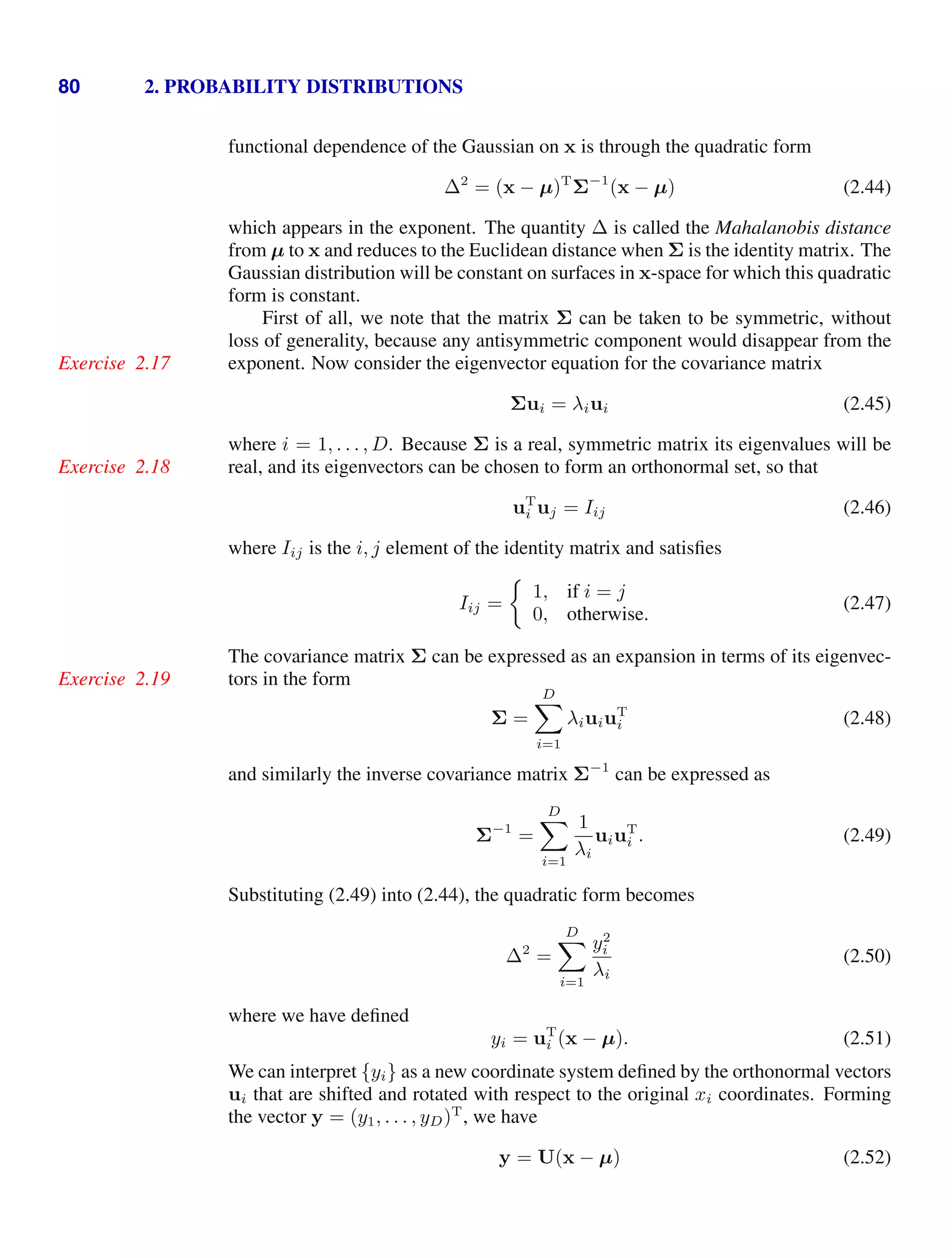
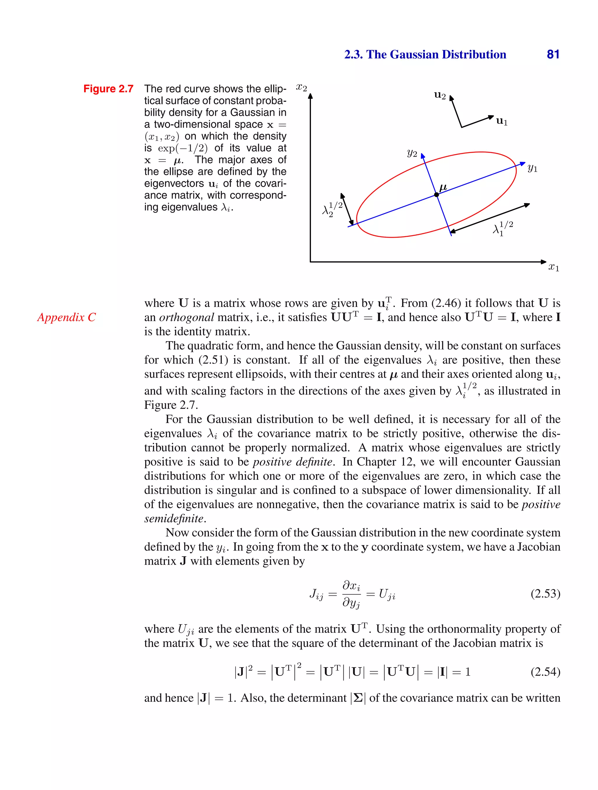
![82 2. PROBABILITY DISTRIBUTIONS
as the product of its eigenvalues, and hence
|Σ|1/2
=
D
j=1
λ
1/2
j . (2.55)
Thus in the yj coordinate system, the Gaussian distribution takes the form
p(y) = p(x)|J| =
D
j=1
1
(2πλj)1/2
exp −
y2
j
2λj
(2.56)
which is the product of D independent univariate Gaussian distributions. The eigen-
vectors therefore define a new set of shifted and rotated coordinates with respect
to which the joint probability distribution factorizes into a product of independent
distributions. The integral of the distribution in the y coordinate system is then
p(y) dy =
D
j=1
∞
−∞
1
(2πλj)1/2
exp −
y2
j
2λj
dyj = 1 (2.57)
where we have used the result (1.48) for the normalization of the univariate Gaussian.
This confirms that the multivariate Gaussian (2.43) is indeed normalized.
We now look at the moments of the Gaussian distribution and thereby provide an
interpretation of the parameters µ and Σ. The expectation of x under the Gaussian
distribution is given by
E[x] =
1
(2π)D/2
1
|Σ|1/2
exp −
1
2
(x − µ)T
Σ−1
(x − µ) x dx
=
1
(2π)D/2
1
|Σ|1/2
exp −
1
2
zT
Σ−1
z (z + µ) dz (2.58)
where we have changed variables using z = x − µ. We now note that the exponent
is an even function of the components of z and, because the integrals over these are
taken over the range (−∞, ∞), the term in z in the factor (z + µ) will vanish by
symmetry. Thus
E[x] = µ (2.59)
and so we refer to µ as the mean of the Gaussian distribution.
We now consider second order moments of the Gaussian. In the univariate case,
we considered the second order moment given by E[x2
]. For the multivariate Gaus-
sian, there are D2
second order moments given by E[xixj], which we can group
together to form the matrix E[xxT
]. This matrix can be written as
E[xxT
] =
1
(2π)D/2
1
|Σ|1/2
exp −
1
2
(x − µ)T
Σ−1
(x − µ) xxT
dx
=
1
(2π)D/2
1
|Σ|1/2
exp −
1
2
zT
Σ−1
z (z + µ)(z + µ)T
dz](https://image.slidesharecdn.com/bishop-patternrecognitionandmachinelearning-230316082240-9af1cdaa/75/Bishop-Pattern-Recognition-and-Machine-Learning-pdf-100-2048.jpg)
![2.3. The Gaussian Distribution 83
where again we have changed variables using z = x − µ. Note that the cross-terms
involving µzT
and µT
z will again vanish by symmetry. The term µµT
is constant
and can be taken outside the integral, which itself is unity because the Gaussian
distribution is normalized. Consider the term involving zzT
. Again, we can make
use of the eigenvector expansion of the covariance matrix given by (2.45), together
with the completeness of the set of eigenvectors, to write
z =
D
j=1
yjuj (2.60)
where yj = uT
j z, which gives
1
(2π)D/2
1
|Σ|1/2
exp −
1
2
zT
Σ−1
z zzT
dz
=
1
(2π)D/2
1
|Σ|1/2
D
i=1
D
j=1
uiuT
j
exp
−
D
k=1
y2
k
2λk
yiyj dy
=
D
i=1
uiuT
i λi = Σ (2.61)
where we have made use of the eigenvector equation (2.45), together with the fact
that the integral on the right-hand side of the middle line vanishes by symmetry
unless i = j, and in the final line we have made use of the results (1.50) and (2.55),
together with (2.48). Thus we have
E[xxT
] = µµT
+ Σ. (2.62)
For single random variables, we subtracted the mean before taking second mo-
ments in order to define a variance. Similarly, in the multivariate case it is again
convenient to subtract off the mean, giving rise to the covariance of a random vector
x defined by
cov[x] = E
(x − E[x])(x − E[x])T
. (2.63)
For the specific case of a Gaussian distribution, we can make use of E[x] = µ,
together with the result (2.62), to give
cov[x] = Σ. (2.64)
Because the parameter matrix Σ governs the covariance of x under the Gaussian
distribution, it is called the covariance matrix.
Although the Gaussian distribution (2.43) is widely used as a density model, it
suffers from some significant limitations. Consider the number of free parameters in
the distribution. A general symmetric covariance matrix Σ will have D(D + 1)/2
independent parameters, and there are another D independent parameters in µ, giv-
Exercise 2.21
ing D(D + 3)/2 parameters in total. For large D, the total number of parameters](https://image.slidesharecdn.com/bishop-patternrecognitionandmachinelearning-230316082240-9af1cdaa/75/Bishop-Pattern-Recognition-and-Machine-Learning-pdf-101-2048.jpg)
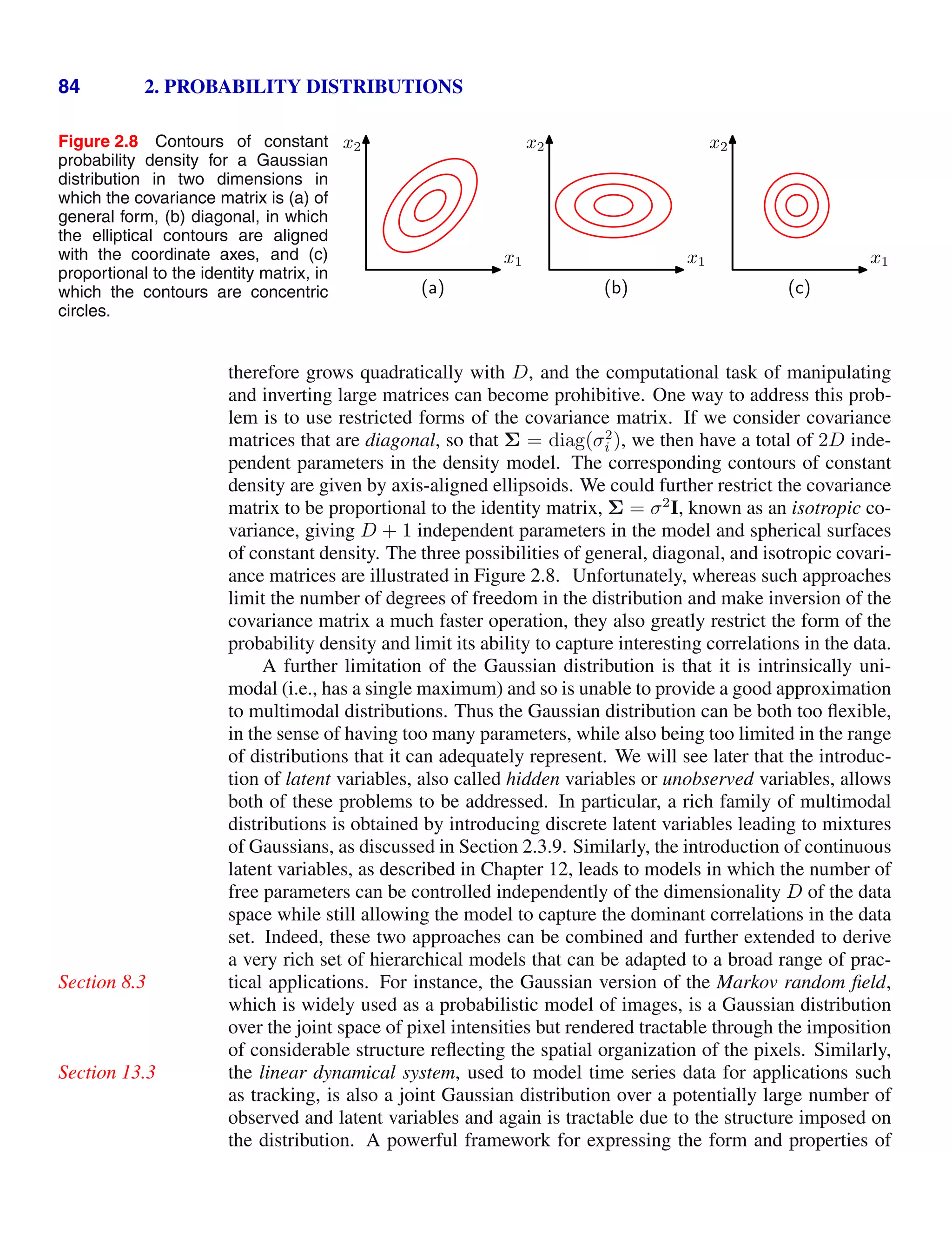
![2.3. The Gaussian Distribution 89
(2.70) that depend on xa, we obtain
1
2
[Λbbµb − Λba(xa − µa)]
T
Λ−1
bb [Λbbµb − Λba(xa − µa)]
−
1
2
xT
a Λaaxa + xT
a (Λaaµa + Λabµb) + const
= −
1
2
xT
a (Λaa − ΛabΛ−1
bb Λba)xa
+xT
a (Λaa − ΛabΛ−1
bb Λba)−1
µa + const (2.87)
where ‘const’ denotes quantities independent of xa. Again, by comparison with
(2.71), we see that the covariance of the marginal distribution of p(xa) is given by
Σa = (Λaa − ΛabΛ−1
bb Λba)−1
. (2.88)
Similarly, the mean is given by
Σa(Λaa − ΛabΛ−1
bb Λba)µa = µa (2.89)
where we have used (2.88). The covariance in (2.88) is expressed in terms of the
partitioned precision matrix given by (2.69). We can rewrite this in terms of the
corresponding partitioning of the covariance matrix given by (2.67), as we did for
the conditional distribution. These partitioned matrices are related by
Λaa Λab
Λba Λbb
−1
=
Σaa Σab
Σba Σbb
(2.90)
Making use of (2.76), we then have
Λaa − ΛabΛ−1
bb Λba
−1
= Σaa. (2.91)
Thus we obtain the intuitively satisfying result that the marginal distribution p(xa)
has mean and covariance given by
E[xa] = µa (2.92)
cov[xa] = Σaa. (2.93)
We see that for a marginal distribution, the mean and covariance are most simply ex-
pressed in terms of the partitioned covariance matrix, in contrast to the conditional
distribution for which the partitioned precision matrix gives rise to simpler expres-
sions.
Our results for the marginal and conditional distributions of a partitioned Gaus-
sian are summarized below.
Partitioned Gaussians
Given a joint Gaussian distribution N(x|µ, Σ) with Λ ≡ Σ−1
and
x =
xa
xb
, µ =
µa
µb
(2.94)](https://image.slidesharecdn.com/bishop-patternrecognitionandmachinelearning-230316082240-9af1cdaa/75/Bishop-Pattern-Recognition-and-Machine-Learning-pdf-107-2048.jpg)
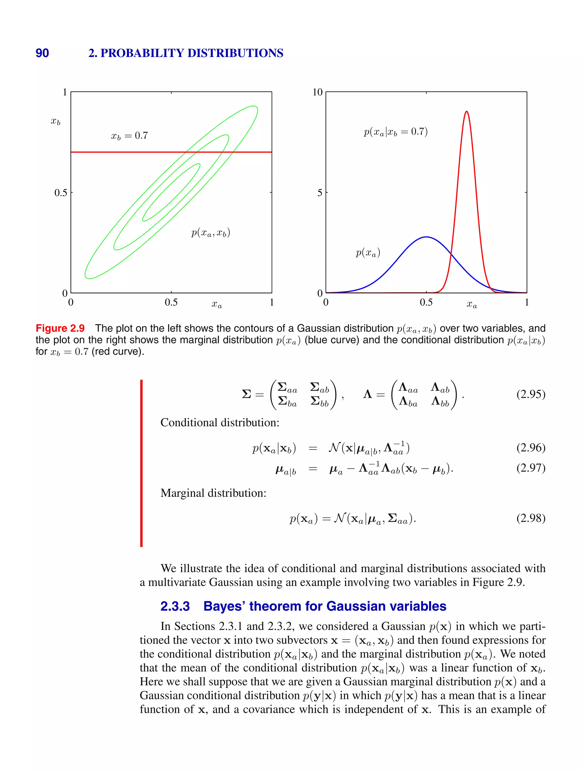
![2.3. The Gaussian Distribution 91
a linear Gaussian model (Roweis and Ghahramani, 1999), which we shall study in
greater generality in Section 8.1.4. We wish to find the marginal distribution p(y)
and the conditional distribution p(x|y). This is a problem that will arise frequently
in subsequent chapters, and it will prove convenient to derive the general results here.
We shall take the marginal and conditional distributions to be
p(x) = N x|µ, Λ−1
(2.99)
p(y|x) = N y|Ax + b, L−1
(2.100)
where µ, A, and b are parameters governing the means, and Λ and L are precision
matrices. If x has dimensionality M and y has dimensionality D, then the matrix A
has size D × M.
First we find an expression for the joint distribution over x and y. To do this, we
define
z =
x
y
(2.101)
and then consider the log of the joint distribution
ln p(z) = ln p(x) + ln p(y|x)
= −
1
2
(x − µ)T
Λ(x − µ)
−
1
2
(y − Ax − b)T
L(y − Ax − b) + const (2.102)
where ‘const’ denotes terms independent of x and y. As before, we see that this is a
quadratic function of the components of z, and hence p(z) is Gaussian distribution.
To find the precision of this Gaussian, we consider the second order terms in (2.102),
which can be written as
−
1
2
xT
(Λ + AT
LA)x −
1
2
yT
Ly +
1
2
yT
LAx +
1
2
xT
AT
Ly
= −
1
2
x
y
T
Λ + AT
LA −AT
L
−LA L
x
y
= −
1
2
zT
Rz (2.103)
and so the Gaussian distribution over z has precision (inverse covariance) matrix
given by
R =
Λ + AT
LA −AT
L
−LA L
. (2.104)
The covariance matrix is found by taking the inverse of the precision, which can be
done using the matrix inversion formula (2.76) to give
Exercise 2.29
cov[z] = R−1
=
Λ−1
Λ−1
AT
AΛ−1
L−1
+ AΛ−1
AT
. (2.105)](https://image.slidesharecdn.com/bishop-patternrecognitionandmachinelearning-230316082240-9af1cdaa/75/Bishop-Pattern-Recognition-and-Machine-Learning-pdf-109-2048.jpg)
![92 2. PROBABILITY DISTRIBUTIONS
Similarly, we can find the mean of the Gaussian distribution over z by identify-
ing the linear terms in (2.102), which are given by
xT
Λµ − xT
AT
Lb + yT
Lb =
x
y
T
Λµ − AT
Lb
Lb
. (2.106)
Using our earlier result (2.71) obtained by completing the square over the quadratic
form of a multivariate Gaussian, we find that the mean of z is given by
E[z] = R−1
Λµ − AT
Lb
Lb
. (2.107)
Making use of (2.105), we then obtain
Exercise 2.30
E[z] =
µ
Aµ + b
. (2.108)
Next we find an expression for the marginal distribution p(y) in which we have
marginalized over x. Recall that the marginal distribution over a subset of the com-
ponents of a Gaussian random vector takes a particularly simple form when ex-
pressed in terms of the partitioned covariance matrix. Specifically, its mean and
Section 2.3
covariance are given by (2.92) and (2.93), respectively. Making use of (2.105) and
(2.108) we see that the mean and covariance of the marginal distribution p(y) are
given by
E[y] = Aµ + b (2.109)
cov[y] = L−1
+ AΛ−1
AT
. (2.110)
A special case of this result is when A = I, in which case it reduces to the convolu-
tion of two Gaussians, for which we see that the mean of the convolution is the sum
of the mean of the two Gaussians, and the covariance of the convolution is the sum
of their covariances.
Finally, we seek an expression for the conditional p(x|y). Recall that the results
for the conditional distribution are most easily expressed in terms of the partitioned
precision matrix, using (2.73) and (2.75). Applying these results to (2.105) and
Section 2.3
(2.108) we see that the conditional distribution p(x|y) has mean and covariance
given by
E[x|y] = (Λ + AT
LA)−1
AT
L(y − b) + Λµ
(2.111)
cov[x|y] = (Λ + AT
LA)−1
. (2.112)
The evaluation of this conditional can be seen as an example of Bayes’ theorem.
We can interpret the distribution p(x) as a prior distribution over x. If the variable
y is observed, then the conditional distribution p(x|y) represents the corresponding
posterior distribution over x. Having found the marginal and conditional distribu-
tions, we effectively expressed the joint distribution p(z) = p(x)p(y|x) in the form
p(x|y)p(y). These results are summarized below.](https://image.slidesharecdn.com/bishop-patternrecognitionandmachinelearning-230316082240-9af1cdaa/75/Bishop-Pattern-Recognition-and-Machine-Learning-pdf-110-2048.jpg)
![94 2. PROBABILITY DISTRIBUTIONS
which is the mean of the observed set of data points. The maximization of (2.118)
with respect to Σ is rather more involved. The simplest approach is to ignore the
symmetry constraint and show that the resulting solution is symmetric as required.
Exercise 2.34
Alternative derivations of this result, which impose the symmetry and positive defi-
niteness constraints explicitly, can be found in Magnus and Neudecker (1999). The
result is as expected and takes the form
ΣML =
1
N
N
n=1
(xn − µML)(xn − µML)T
(2.122)
which involves µML because this is the result of a joint maximization with respect
to µ and Σ. Note that the solution (2.121) for µML does not depend on ΣML, and so
we can first evaluate µML and then use this to evaluate ΣML.
If we evaluate the expectations of the maximum likelihood solutions under the
true distribution, we obtain the following results
Exercise 2.35
E[µML] = µ (2.123)
E[ΣML] =
N − 1
N
Σ. (2.124)
We see that the expectation of the maximum likelihood estimate for the mean is equal
to the true mean. However, the maximum likelihood estimate for the covariance has
an expectation that is less than the true value, and hence it is biased. We can correct
this bias by defining a different estimator
Σ given by
Σ =
1
N − 1
N
n=1
(xn − µML)(xn − µML)T
. (2.125)
Clearly from (2.122) and (2.124), the expectation of
Σ is equal to Σ.
2.3.5 Sequential estimation
Our discussion of the maximum likelihood solution for the parameters of a Gaus-
sian distribution provides a convenient opportunity to give a more general discussion
of the topic of sequential estimation for maximum likelihood. Sequential methods
allow data points to be processed one at a time and then discarded and are important
for on-line applications, and also where large data sets are involved so that batch
processing of all data points at once is infeasible.
Consider the result (2.121) for the maximum likelihood estimator of the mean
µML, which we will denote by µ
(N)
ML when it is based on N observations. If we](https://image.slidesharecdn.com/bishop-patternrecognitionandmachinelearning-230316082240-9af1cdaa/75/Bishop-Pattern-Recognition-and-Machine-Learning-pdf-112-2048.jpg)
![2.3. The Gaussian Distribution 95
Figure 2.10 A schematic illustration of two correlated ran-
dom variables z and θ, together with the
regression function f(θ) given by the con-
ditional expectation E[z|θ]. The Robbins-
Monro algorithm provides a general sequen-
tial procedure for finding the root θ
of such
functions. θ
z
θ
f(θ)
dissect out the contribution from the final data point xN , we obtain
µ
(N)
ML =
1
N
N
n=1
xn
=
1
N
xN +
1
N
N−1
n=1
xn
=
1
N
xN +
N − 1
N
µ
(N−1)
ML
= µ
(N−1)
ML +
1
N
(xN − µ
(N−1)
ML ). (2.126)
This result has a nice interpretation, as follows. After observing N − 1 data points
we have estimated µ by µ
(N−1)
ML . We now observe data point xN , and we obtain our
revised estimate µ
(N)
ML by moving the old estimate a small amount, proportional to
1/N, in the direction of the ‘error signal’ (xN −µ
(N−1)
ML ). Note that, as N increases,
so the contribution from successive data points gets smaller.
The result (2.126) will clearly give the same answer as the batch result (2.121)
because the two formulae are equivalent. However, we will not always be able to de-
rive a sequential algorithm by this route, and so we seek a more general formulation
of sequential learning, which leads us to the Robbins-Monro algorithm. Consider a
pair of random variables θ and z governed by a joint distribution p(z, θ). The con-
ditional expectation of z given θ defines a deterministic function f(θ) that is given
by
f(θ) ≡ E[z|θ] =
zp(z|θ) dz (2.127)
and is illustrated schematically in Figure 2.10. Functions defined in this way are
called regression functions.
Our goal is to find the root θ
at which f(θ
) = 0. If we had a large data set
of observations of z and θ, then we could model the regression function directly and
then obtain an estimate of its root. Suppose, however, that we observe values of
z one at a time and we wish to find a corresponding sequential estimation scheme
for θ
. The following general procedure for solving such problems was given by](https://image.slidesharecdn.com/bishop-patternrecognitionandmachinelearning-230316082240-9af1cdaa/75/Bishop-Pattern-Recognition-and-Machine-Learning-pdf-113-2048.jpg)
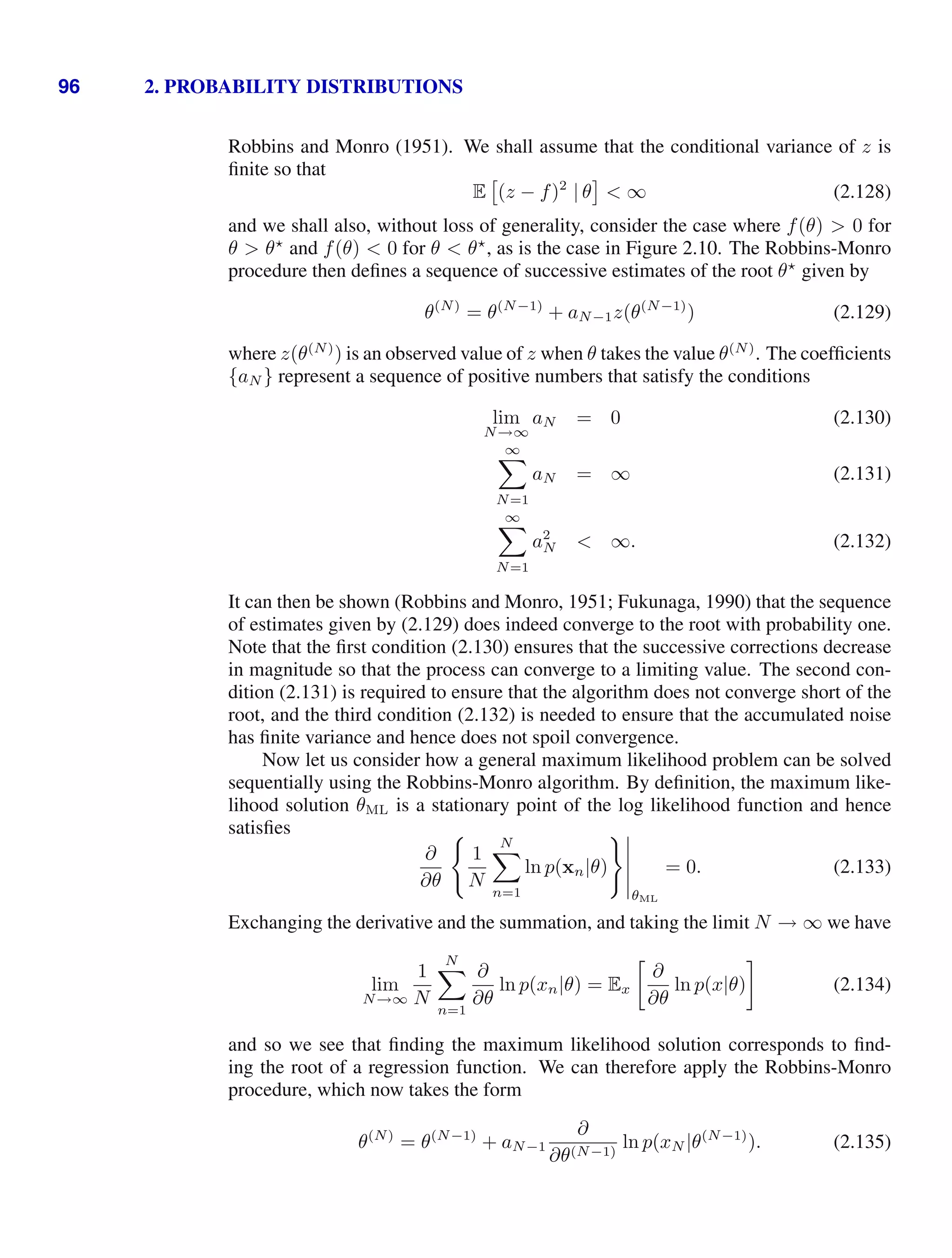
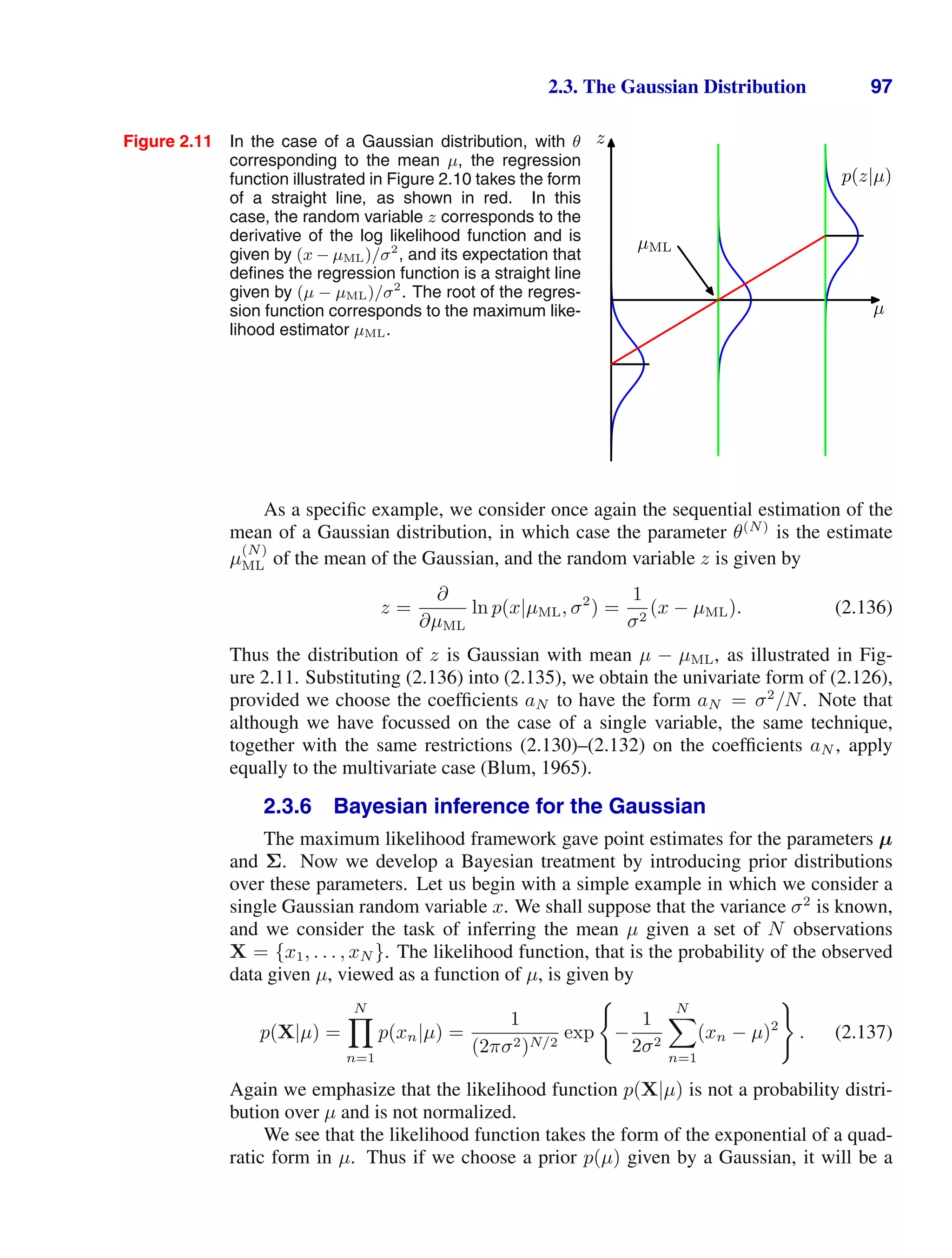
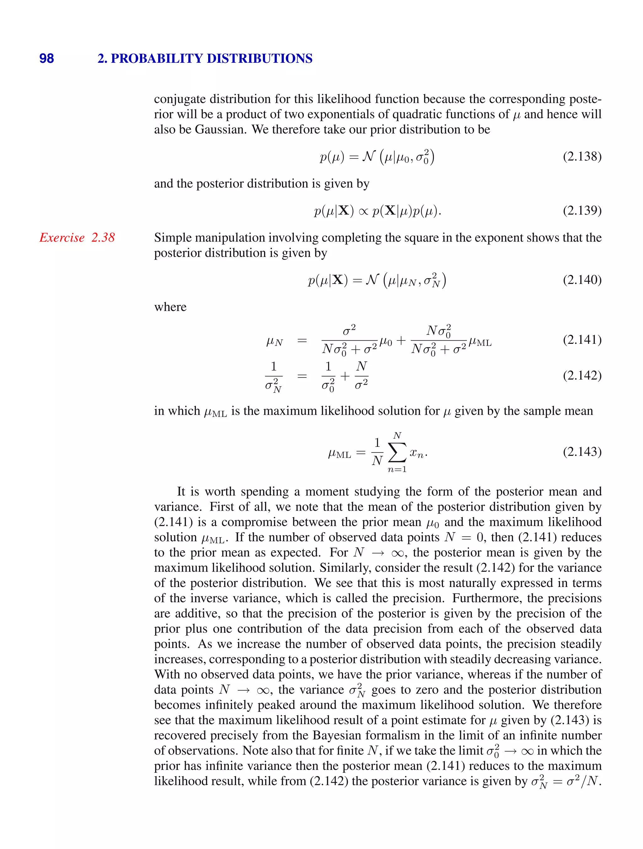
![100 2. PROBABILITY DISTRIBUTIONS
λ
a = 0.1
b = 0.1
0 1 2
0
1
2
λ
a = 1
b = 1
0 1 2
0
1
2
λ
a = 4
b = 6
0 1 2
0
1
2
Figure 2.13 Plot of the gamma distribution Gam(λ|a, b) defined by (2.146) for various values of the parameters
a and b.
The corresponding conjugate prior should therefore be proportional to the product
of a power of λ and the exponential of a linear function of λ. This corresponds to
the gamma distribution which is defined by
Gam(λ|a, b) =
1
Γ(a)
ba
λa−1
exp(−bλ). (2.146)
Here Γ(a) is the gamma function that is defined by (1.141) and that ensures that
(2.146) is correctly normalized. The gamma distribution has a finite integral if a 0,
Exercise 2.41
and the distribution itself is finite if a 1. It is plotted, for various values of a and
b, in Figure 2.13. The mean and variance of the gamma distribution are given by
Exercise 2.42
E[λ] =
a
b
(2.147)
var[λ] =
a
b2
. (2.148)
Consider a prior distribution Gam(λ|a0, b0). If we multiply by the likelihood
function (2.145), then we obtain a posterior distribution
p(λ|X) ∝ λa0−1
λN/2
exp
−b0λ −
λ
2
N
n=1
(xn − µ)2
(2.149)
which we recognize as a gamma distribution of the form Gam(λ|aN , bN ) where
aN = a0 +
N
2
(2.150)
bN = b0 +
1
2
N
n=1
(xn − µ)2
= b0 +
N
2
σ2
ML (2.151)
where σ2
ML is the maximum likelihood estimator of the variance. Note that in (2.149)
there is no need to keep track of the normalization constants in the prior and the
likelihood function because, if required, the correct coefficient can be found at the
end using the normalized form (2.146) for the gamma distribution.](https://image.slidesharecdn.com/bishop-patternrecognitionandmachinelearning-230316082240-9af1cdaa/75/Bishop-Pattern-Recognition-and-Machine-Learning-pdf-118-2048.jpg)
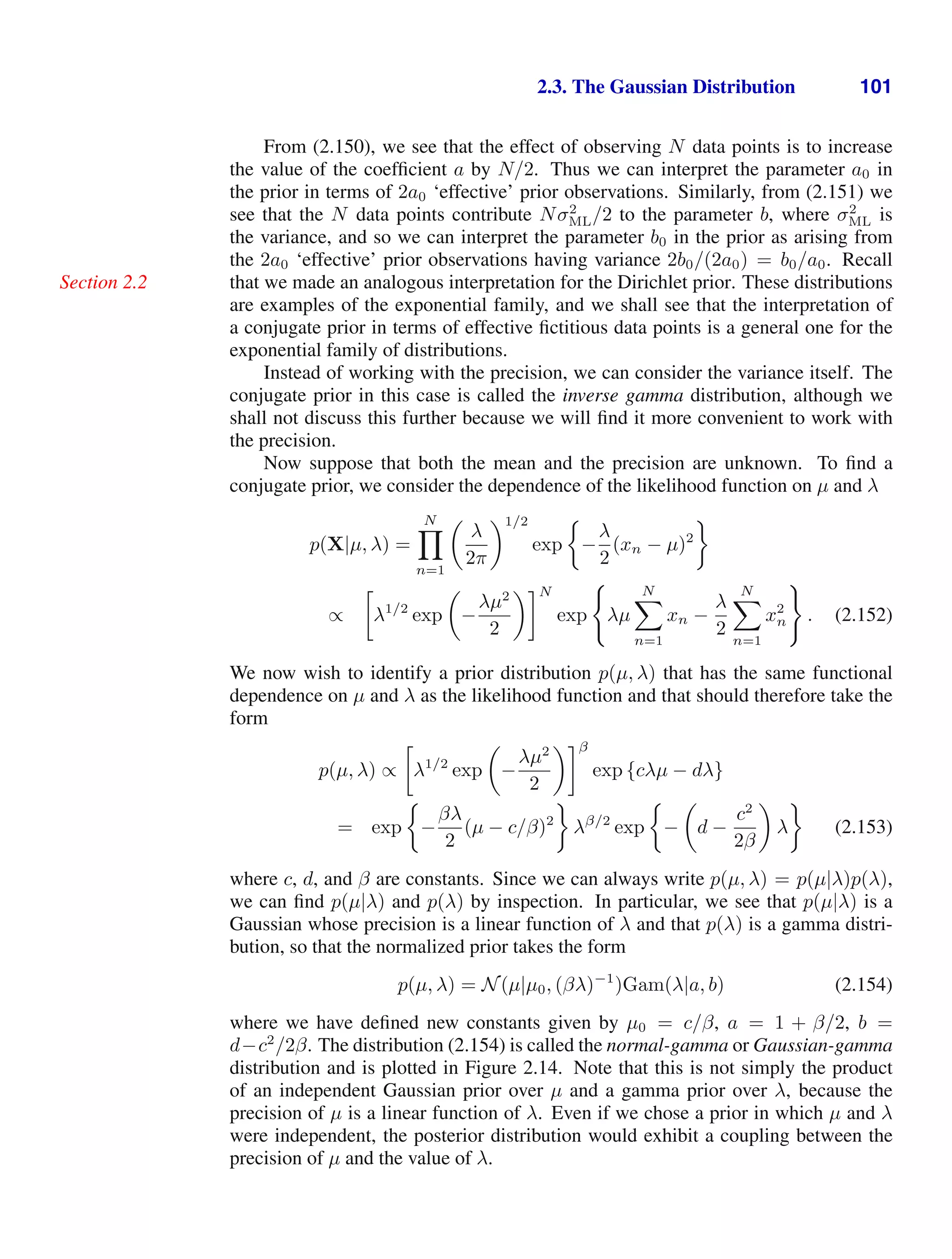
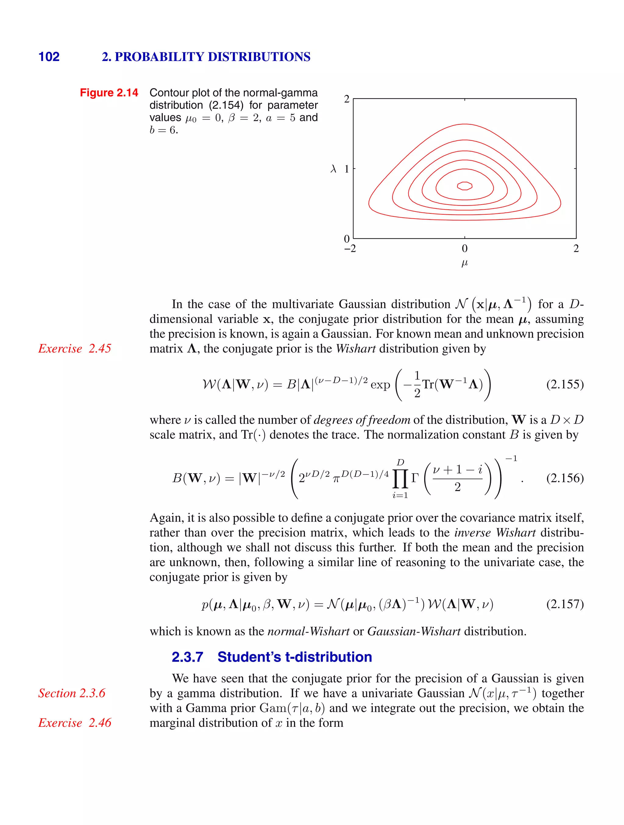
![2.3. The Gaussian Distribution 103
Figure 2.15 Plot of Student’s t-distribution (2.159)
for µ = 0 and λ = 1 for various values
of ν. The limit ν → ∞ corresponds
to a Gaussian distribution with mean
µ and precision λ.
ν → ∞
ν = 1.0
ν = 0.1
−5 0 5
0
0.1
0.2
0.3
0.4
0.5
p(x|µ, a, b) =
∞
0
N(x|µ, τ−1
)Gam(τ|a, b) dτ (2.158)
=
∞
0
ba
e(−bτ)
τa−1
Γ(a)
τ
2π
1/2
exp
−
τ
2
(x − µ)2
dτ
=
ba
Γ(a)
1
2π
1/2
b +
(x − µ)2
2
−a−1/2
Γ(a + 1/2)
where we have made the change of variable z = τ[b + (x − µ)2
/2]. By convention
we define new parameters given by ν = 2a and λ = a/b, in terms of which the
distribution p(x|µ, a, b) takes the form
St(x|µ, λ, ν) =
Γ(ν/2 + 1/2)
Γ(ν/2)
λ
πν
1/2
1 +
λ(x − µ)2
ν
−ν/2−1/2
(2.159)
which is known as Student’s t-distribution. The parameter λ is sometimes called the
precision of the t-distribution, even though it is not in general equal to the inverse
of the variance. The parameter ν is called the degrees of freedom, and its effect is
illustrated in Figure 2.15. For the particular case of ν = 1, the t-distribution reduces
to the Cauchy distribution, while in the limit ν → ∞ the t-distribution St(x|µ, λ, ν)
becomes a Gaussian N(x|µ, λ−1
) with mean µ and precision λ.
Exercise 2.47
From (2.158), we see that Student’s t-distribution is obtained by adding up an
infinite number of Gaussian distributions having the same mean but different preci-
sions. This can be interpreted as an infinite mixture of Gaussians (Gaussian mixtures
will be discussed in detail in Section 2.3.9. The result is a distribution that in gen-
eral has longer ‘tails’ than a Gaussian, as was seen in Figure 2.15. This gives the t-
distribution an important property called robustness, which means that it is much less
sensitive than the Gaussian to the presence of a few data points which are outliers.
The robustness of the t-distribution is illustrated in Figure 2.16, which compares the
maximum likelihood solutions for a Gaussian and a t-distribution. Note that the max-
imum likelihood solution for the t-distribution can be found using the expectation-
maximization (EM) algorithm. Here we see that the effect of a small number of
Exercise 12.24](https://image.slidesharecdn.com/bishop-patternrecognitionandmachinelearning-230316082240-9af1cdaa/75/Bishop-Pattern-Recognition-and-Machine-Learning-pdf-121-2048.jpg)
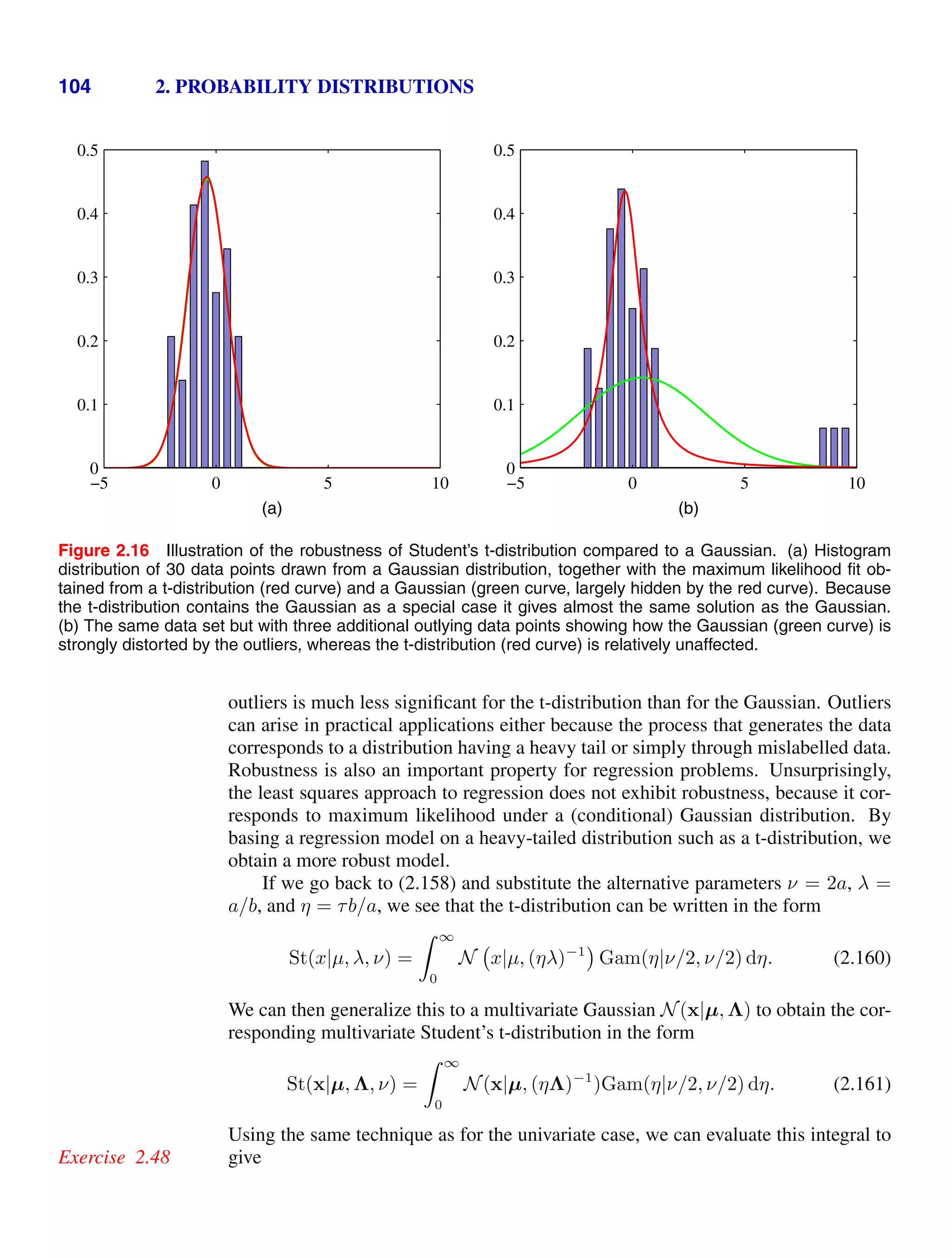
![2.3. The Gaussian Distribution 105
St(x|µ, Λ, ν) =
Γ(D/2 + ν/2)
Γ(ν/2)
|Λ|1/2
(πν)D/2
1 +
∆2
ν
−D/2−ν/2
(2.162)
where D is the dimensionality of x, and ∆2
is the squared Mahalanobis distance
defined by
∆2
= (x − µ)T
Λ(x − µ). (2.163)
This is the multivariate form of Student’s t-distribution and satisfies the following
properties
Exercise 2.49
E[x] = µ, if ν 1 (2.164)
cov[x] =
ν
(ν − 2)
Λ−1
, if ν 2 (2.165)
mode[x] = µ (2.166)
with corresponding results for the univariate case.
2.3.8 Periodic variables
Although Gaussian distributions are of great practical significance, both in their
own right and as building blocks for more complex probabilistic models, there are
situations in which they are inappropriate as density models for continuous vari-
ables. One important case, which arises in practical applications, is that of periodic
variables.
An example of a periodic variable would be the wind direction at a particular
geographical location. We might, for instance, measure values of wind direction on a
number of days and wish to summarize this using a parametric distribution. Another
example is calendar time, where we may be interested in modelling quantities that
are believed to be periodic over 24 hours or over an annual cycle. Such quantities
can conveniently be represented using an angular (polar) coordinate 0 θ 2π.
We might be tempted to treat periodic variables by choosing some direction
as the origin and then applying a conventional distribution such as the Gaussian.
Such an approach, however, would give results that were strongly dependent on the
arbitrary choice of origin. Suppose, for instance, that we have two observations at
θ1 = 1◦
and θ2 = 359◦
, and we model them using a standard univariate Gaussian
distribution. If we choose the origin at 0◦
, then the sample mean of this data set
will be 180◦
with standard deviation 179◦
, whereas if we choose the origin at 180◦
,
then the mean will be 0◦
and the standard deviation will be 1◦
. We clearly need to
develop a special approach for the treatment of periodic variables.
Let us consider the problem of evaluating the mean of a set of observations
D = {θ1, . . . , θN } of a periodic variable. From now on, we shall assume that θ is
measured in radians. We have already seen that the simple average (θ1+· · ·+θN )/N
will be strongly coordinate dependent. To find an invariant measure of the mean, we
note that the observations can be viewed as points on the unit circle and can therefore
be described instead by two-dimensional unit vectors x1, . . . , xN where xn = 1
for n = 1, . . . , N, as illustrated in Figure 2.17. We can average the vectors {xn}](https://image.slidesharecdn.com/bishop-patternrecognitionandmachinelearning-230316082240-9af1cdaa/75/Bishop-Pattern-Recognition-and-Machine-Learning-pdf-123-2048.jpg)
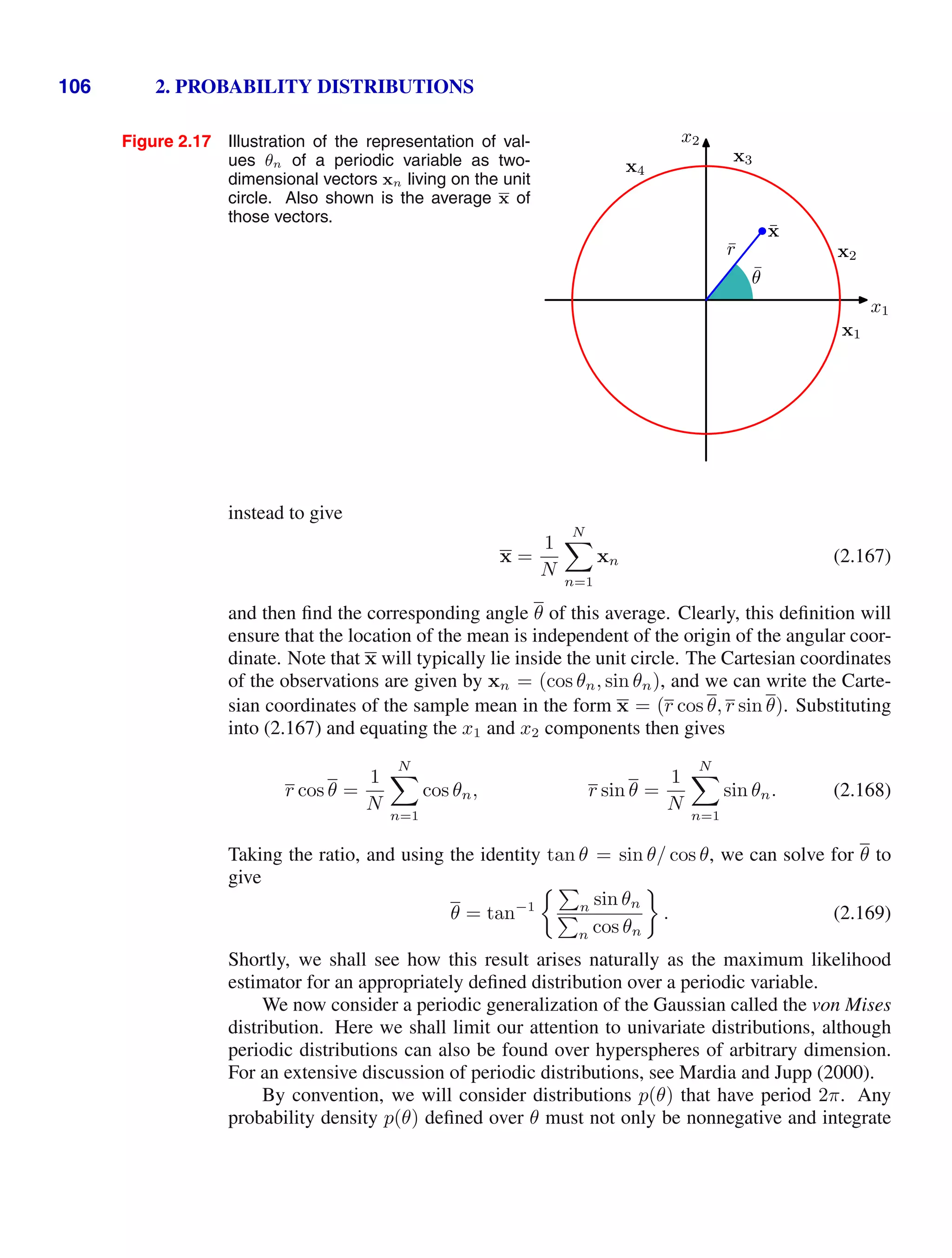

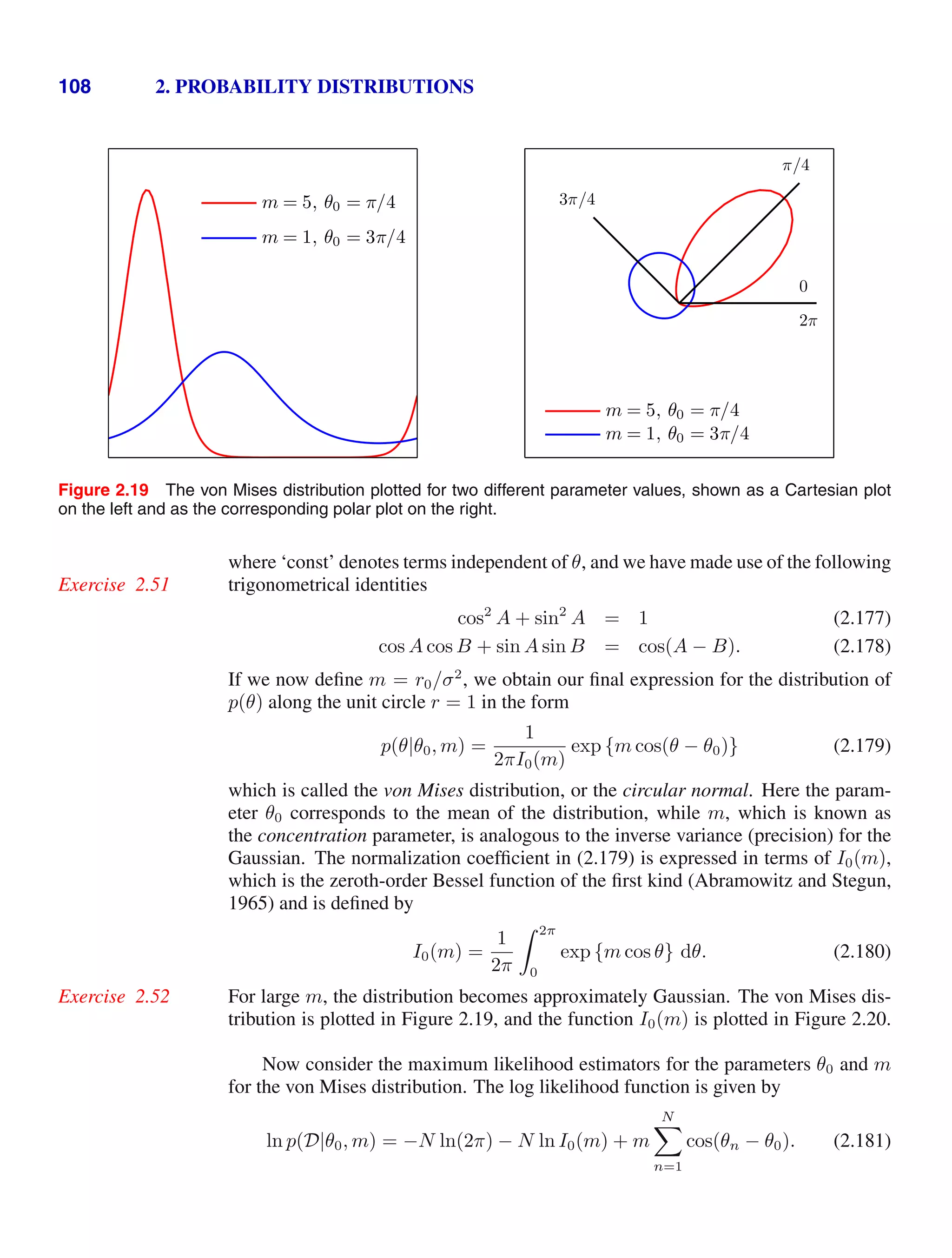
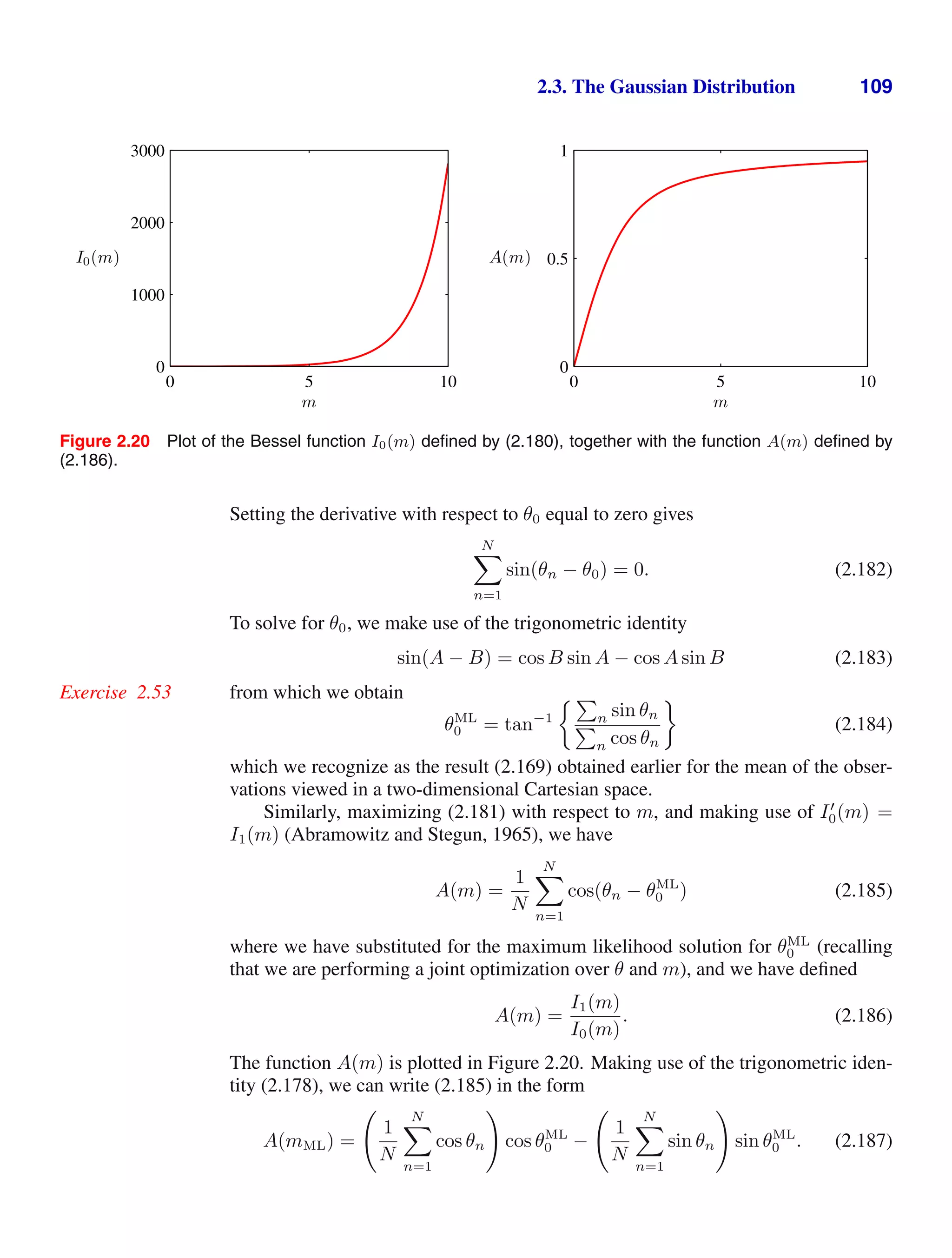
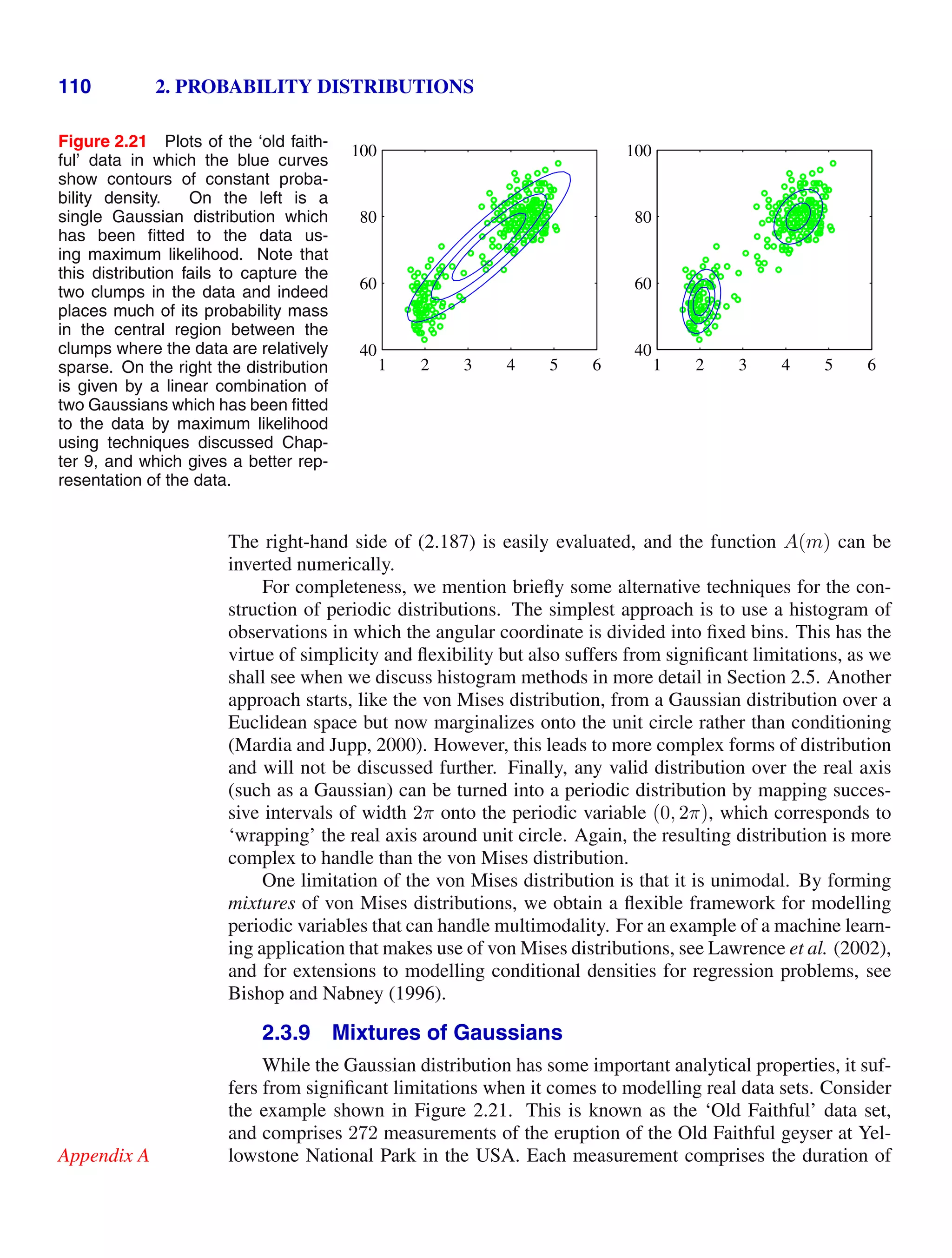
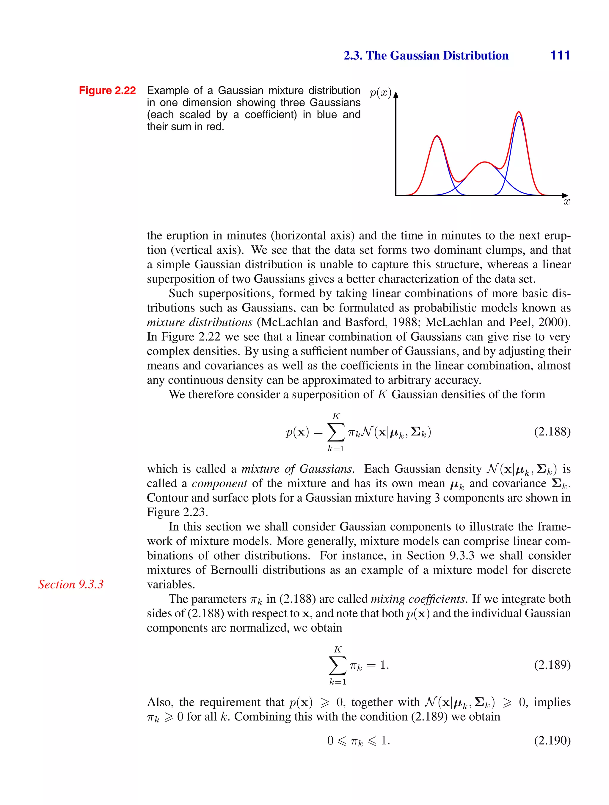
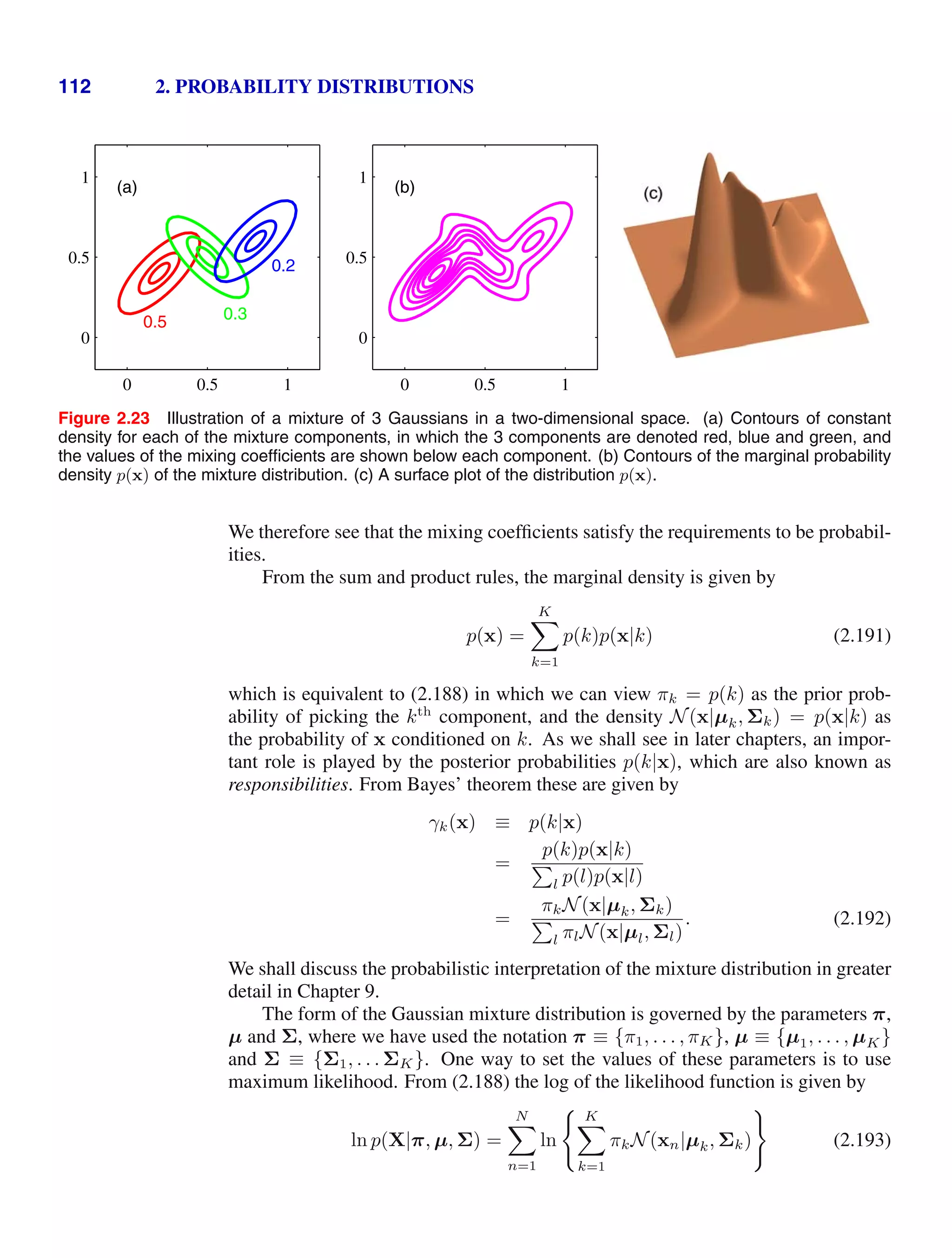
![116 2. PROBABILITY DISTRIBUTIONS
which, after some simple rearrangement, can be cast in the standard exponential
family form (2.194) with
Exercise 2.57
η =
µ/σ2
−1/2σ2
(2.220)
u(x) =
x
x2
(2.221)
h(x) = (2π)−1/2
(2.222)
g(η) = (−2η2)1/2
exp
η2
1
4η2
. (2.223)
2.4.1 Maximum likelihood and sufficient statistics
Let us now consider the problem of estimating the parameter vector η in the gen-
eral exponential family distribution (2.194) using the technique of maximum likeli-
hood. Taking the gradient of both sides of (2.195) with respect to η, we have
∇g(η)
h(x) exp
ηT
u(x)
dx
+ g(η)
h(x) exp
ηT
u(x)
u(x) dx = 0. (2.224)
Rearranging, and making use again of (2.195) then gives
−
1
g(η)
∇g(η) = g(η)
h(x) exp
ηT
u(x)
u(x) dx = E[u(x)] (2.225)
where we have used (2.194). We therefore obtain the result
−∇ ln g(η) = E[u(x)]. (2.226)
Note that the covariance of u(x) can be expressed in terms of the second derivatives
of g(η), and similarly for higher order moments. Thus, provided we can normalize a
Exercise 2.58
distribution from the exponential family, we can always find its moments by simple
differentiation.
Now consider a set of independent identically distributed data denoted by X =
{x1, . . . , xn}, for which the likelihood function is given by
p(X|η) =
N
n=1
h(xn)
g(η)N
exp
ηT
N
n=1
u(xn)
. (2.227)
Setting the gradient of ln p(X|η) with respect to η to zero, we get the following
condition to be satisfied by the maximum likelihood estimator ηML
−∇ ln g(ηML) =
1
N
N
n=1
u(xn) (2.228)](https://image.slidesharecdn.com/bishop-patternrecognitionandmachinelearning-230316082240-9af1cdaa/75/Bishop-Pattern-Recognition-and-Machine-Learning-pdf-134-2048.jpg)
![2.4. The Exponential Family 117
which can in principle be solved to obtain ηML. We see that the solution for the
maximum likelihood estimator depends on the data only through
n u(xn), which
is therefore called the sufficient statistic of the distribution (2.194). We do not need
to store the entire data set itself but only the value of the sufficient statistic. For
the Bernoulli distribution, for example, the function u(x) is given just by x and
so we need only keep the sum of the data points {xn}, whereas for the Gaussian
u(x) = (x, x2
)T
, and so we should keep both the sum of {xn} and the sum of {x2
n}.
If we consider the limit N → ∞, then the right-hand side of (2.228) becomes
E[u(x)], and so by comparing with (2.226) we see that in this limit ηML will equal
the true value η.
In fact, this sufficiency property holds also for Bayesian inference, although
we shall defer discussion of this until Chapter 8 when we have equipped ourselves
with the tools of graphical models and can thereby gain a deeper insight into these
important concepts.
2.4.2 Conjugate priors
We have already encountered the concept of a conjugate prior several times, for
example in the context of the Bernoulli distribution (for which the conjugate prior
is the beta distribution) or the Gaussian (where the conjugate prior for the mean is
a Gaussian, and the conjugate prior for the precision is the Wishart distribution). In
general, for a given probability distribution p(x|η), we can seek a prior p(η) that is
conjugate to the likelihood function, so that the posterior distribution has the same
functional form as the prior. For any member of the exponential family (2.194), there
exists a conjugate prior that can be written in the form
p(η|χ, ν) = f(χ, ν)g(η)ν
exp
νηT
χ
(2.229)
where f(χ, ν) is a normalization coefficient, and g(η) is the same function as ap-
pears in (2.194). To see that this is indeed conjugate, let us multiply the prior (2.229)
by the likelihood function (2.227) to obtain the posterior distribution, up to a nor-
malization coefficient, in the form
p(η|X, χ, ν) ∝ g(η)ν+N
exp
ηT
N
n=1
u(xn) + νχ
. (2.230)
This again takes the same functional form as the prior (2.229), confirming conjugacy.
Furthermore, we see that the parameter ν can be interpreted as a effective number of
pseudo-observations in the prior, each of which has a value for the sufficient statistic
u(x) given by χ.
2.4.3 Noninformative priors
In some applications of probabilistic inference, we may have prior knowledge
that can be conveniently expressed through the prior distribution. For example, if
the prior assigns zero probability to some value of variable, then the posterior dis-
tribution will necessarily also assign zero probability to that value, irrespective of](https://image.slidesharecdn.com/bishop-patternrecognitionandmachinelearning-230316082240-9af1cdaa/75/Bishop-Pattern-Recognition-and-Machine-Learning-pdf-135-2048.jpg)
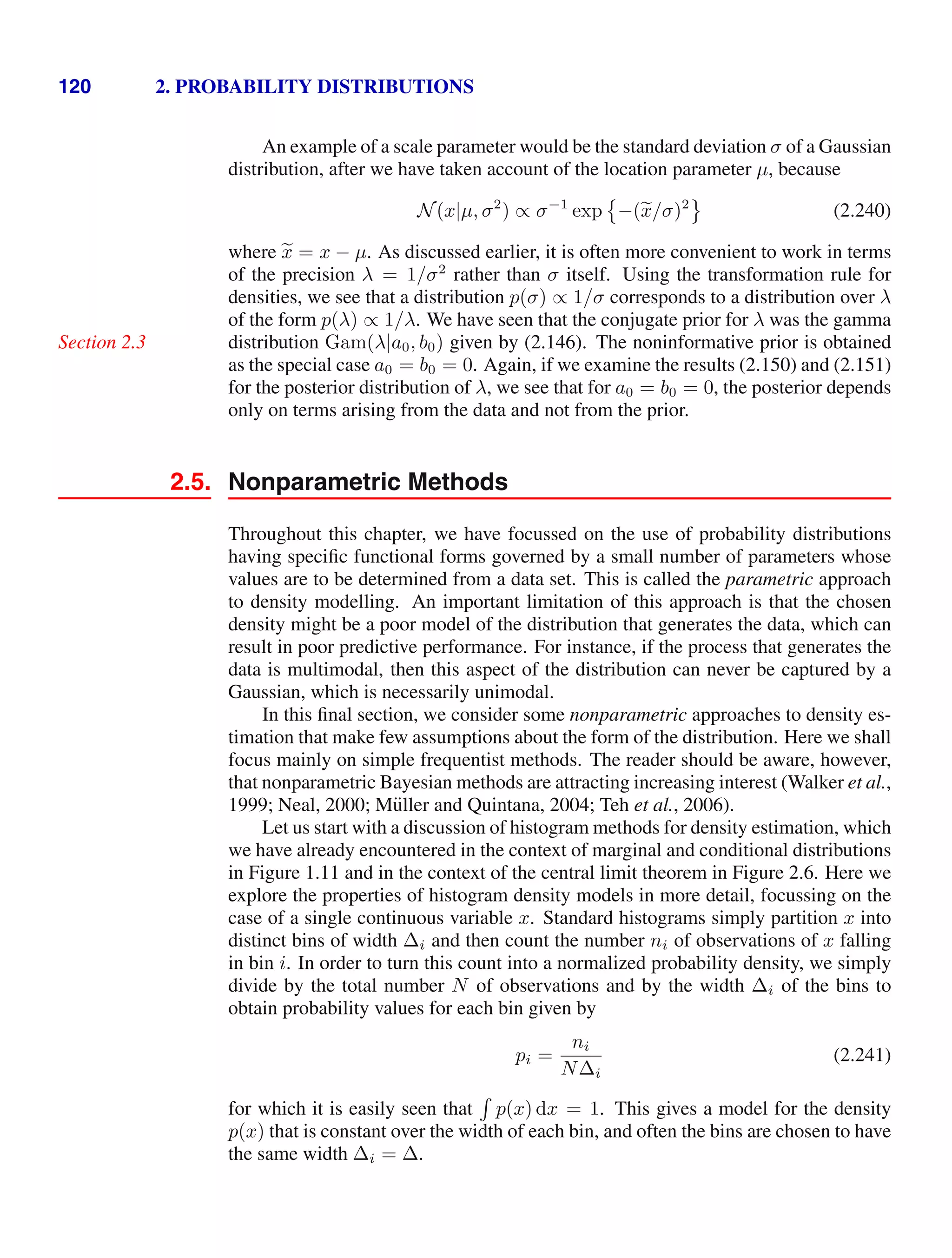
![122 2. PROBABILITY DISTRIBUTIONS
this neighbourhood property was defined by the bins, and there is a natural ‘smooth-
ing’ parameter describing the spatial extent of the local region, in this case the bin
width. Second, the value of the smoothing parameter should be neither too large nor
too small in order to obtain good results. This is reminiscent of the choice of model
complexity in polynomial curve fitting discussed in Chapter 1 where the degree M
of the polynomial, or alternatively the value α of the regularization parameter, was
optimal for some intermediate value, neither too large nor too small. Armed with
these insights, we turn now to a discussion of two widely used nonparametric tech-
niques for density estimation, kernel estimators and nearest neighbours, which have
better scaling with dimensionality than the simple histogram model.
2.5.1 Kernel density estimators
Let us suppose that observations are being drawn from some unknown probabil-
ity density p(x) in some D-dimensional space, which we shall take to be Euclidean,
and we wish to estimate the value of p(x). From our earlier discussion of locality,
let us consider some small region R containing x. The probability mass associated
with this region is given by
P =
R
p(x) dx. (2.242)
Now suppose that we have collected a data set comprising N observations drawn
from p(x). Because each data point has a probability P of falling within R, the total
number K of points that lie inside R will be distributed according to the binomial
distribution
Section 2.1
Bin(K|N, P) =
N!
K!(N − K)!
PK
(1 − P)1−K
. (2.243)
Using (2.11), we see that the mean fraction of points falling inside the region is
E[K/N] = P, and similarly using (2.12) we see that the variance around this mean
is var[K/N] = P(1 − P)/N. For large N, this distribution will be sharply peaked
around the mean and so
K NP. (2.244)
If, however, we also assume that the region R is sufficiently small that the probability
density p(x) is roughly constant over the region, then we have
P p(x)V (2.245)
where V is the volume of R. Combining (2.244) and (2.245), we obtain our density
estimate in the form
p(x) =
K
NV
. (2.246)
Note that the validity of (2.246) depends on two contradictory assumptions, namely
that the region R be sufficiently small that the density is approximately constant over
the region and yet sufficiently large (in relation to the value of that density) that the
number K of points falling inside the region is sufficient for the binomial distribution
to be sharply peaked.](https://image.slidesharecdn.com/bishop-patternrecognitionandmachinelearning-230316082240-9af1cdaa/75/Bishop-Pattern-Recognition-and-Machine-Learning-pdf-140-2048.jpg)
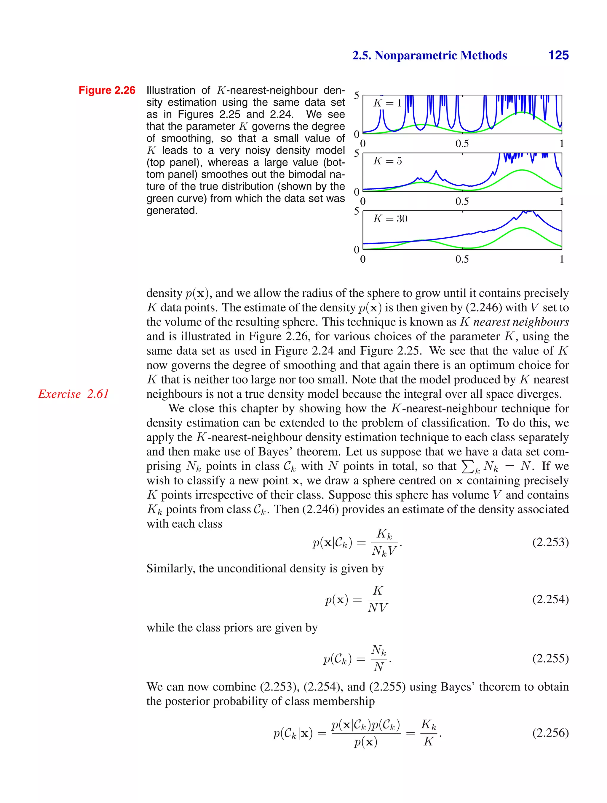
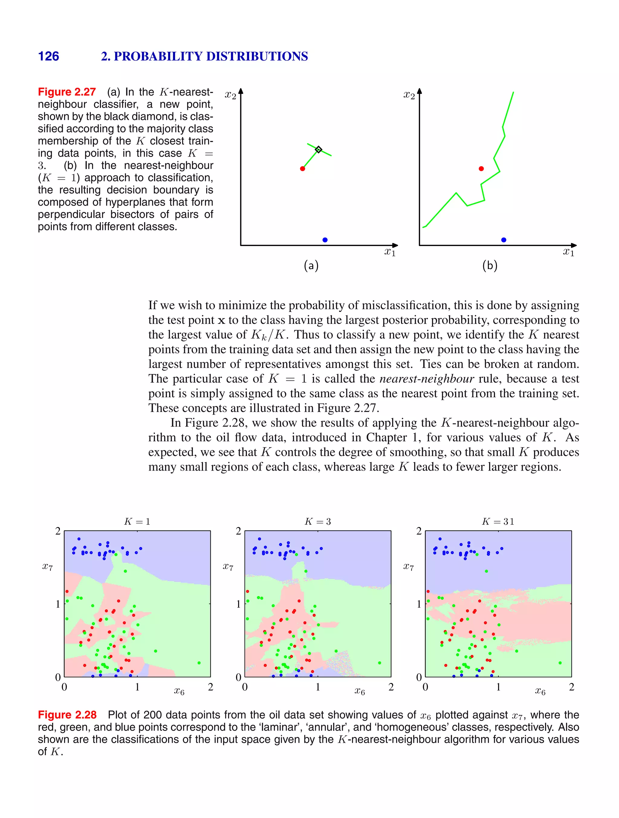
![Exercises 127
An interesting property of the nearest-neighbour (K = 1) classifier is that, in the
limit N → ∞, the error rate is never more than twice the minimum achievable error
rate of an optimal classifier, i.e., one that uses the true class distributions (Cover and
Hart, 1967) .
As discussed so far, both the K-nearest-neighbour method, and the kernel den-
sity estimator, require the entire training data set to be stored, leading to expensive
computation if the data set is large. This effect can be offset, at the expense of some
additional one-off computation, by constructing tree-based search structures to allow
(approximate) near neighbours to be found efficiently without doing an exhaustive
search of the data set. Nevertheless, these nonparametric methods are still severely
limited. On the other hand, we have seen that simple parametric models are very
restricted in terms of the forms of distribution that they can represent. We therefore
need to find density models that are very flexible and yet for which the complexity
of the models can be controlled independently of the size of the training set, and we
shall see in subsequent chapters how to achieve this.
Exercises
2.1 ( ) www Verify that the Bernoulli distribution (2.2) satisfies the following prop-
erties
1
x=0
p(x|µ) = 1 (2.257)
E[x] = µ (2.258)
var[x] = µ(1 − µ). (2.259)
Show that the entropy H[x] of a Bernoulli distributed random binary variable x is
given by
H[x] = −µ ln µ − (1 − µ) ln(1 − µ). (2.260)
2.2 ( ) The form of the Bernoulli distribution given by (2.2) is not symmetric be-
tween the two values of x. In some situations, it will be more convenient to use an
equivalent formulation for which x ∈ {−1, 1}, in which case the distribution can be
written
p(x|µ) =
1 − µ
2
(1−x)/2
1 + µ
2
(1+x)/2
(2.261)
where µ ∈ [−1, 1]. Show that the distribution (2.261) is normalized, and evaluate its
mean, variance, and entropy.
2.3 ( ) www In this exercise, we prove that the binomial distribution (2.9) is nor-
malized. First use the definition (2.10) of the number of combinations of m identical
objects chosen from a total of N to show that
N
m
+
N
m − 1
=
N + 1
m
. (2.262)](https://image.slidesharecdn.com/bishop-patternrecognitionandmachinelearning-230316082240-9af1cdaa/75/Bishop-Pattern-Recognition-and-Machine-Learning-pdf-145-2048.jpg)
![128 2. PROBABILITY DISTRIBUTIONS
Use this result to prove by induction the following result
(1 + x)N
=
N
m=0
N
m
xm
(2.263)
which is known as the binomial theorem, and which is valid for all real values of x.
Finally, show that the binomial distribution is normalized, so that
N
m=0
N
m
µm
(1 − µ)N−m
= 1 (2.264)
which can be done by first pulling out a factor (1 − µ)N
out of the summation and
then making use of the binomial theorem.
2.4 ( ) Show that the mean of the binomial distribution is given by (2.11). To do this,
differentiate both sides of the normalization condition (2.264) with respect to µ and
then rearrange to obtain an expression for the mean of n. Similarly, by differentiating
(2.264) twice with respect to µ and making use of the result (2.11) for the mean of
the binomial distribution prove the result (2.12) for the variance of the binomial.
2.5 ( ) www In this exercise, we prove that the beta distribution, given by (2.13), is
correctly normalized, so that (2.14) holds. This is equivalent to showing that
1
0
µa−1
(1 − µ)b−1
dµ =
Γ(a)Γ(b)
Γ(a + b)
. (2.265)
From the definition (1.141) of the gamma function, we have
Γ(a)Γ(b) =
∞
0
exp(−x)xa−1
dx
∞
0
exp(−y)yb−1
dy. (2.266)
Use this expression to prove (2.265) as follows. First bring the integral over y inside
the integrand of the integral over x, next make the change of variable t = y + x
where x is fixed, then interchange the order of the x and t integrations, and finally
make the change of variable x = tµ where t is fixed.
2.6 ( ) Make use of the result (2.265) to show that the mean, variance, and mode of the
beta distribution (2.13) are given respectively by
E[µ] =
a
a + b
(2.267)
var[µ] =
ab
(a + b)2(a + b + 1)
(2.268)
mode[µ] =
a − 1
a + b − 2
. (2.269)](https://image.slidesharecdn.com/bishop-patternrecognitionandmachinelearning-230316082240-9af1cdaa/75/Bishop-Pattern-Recognition-and-Machine-Learning-pdf-146-2048.jpg)
![Exercises 129
2.7 ( ) Consider a binomial random variable x given by (2.9), with prior distribution
for µ given by the beta distribution (2.13), and suppose we have observed m occur-
rences of x = 1 and l occurrences of x = 0. Show that the posterior mean value of x
lies between the prior mean and the maximum likelihood estimate for µ. To do this,
show that the posterior mean can be written as λ times the prior mean plus (1 − λ)
times the maximum likelihood estimate, where 0 λ 1. This illustrates the con-
cept of the posterior distribution being a compromise between the prior distribution
and the maximum likelihood solution.
2.8 ( ) Consider two variables x and y with joint distribution p(x, y). Prove the follow-
ing two results
E[x] = Ey [Ex[x|y]] (2.270)
var[x] = Ey [varx[x|y]] + vary [Ex[x|y]] . (2.271)
Here Ex[x|y] denotes the expectation of x under the conditional distribution p(x|y),
with a similar notation for the conditional variance.
2.9 ( ) www . In this exercise, we prove the normalization of the Dirichlet dis-
tribution (2.38) using induction. We have already shown in Exercise 2.5 that the
beta distribution, which is a special case of the Dirichlet for M = 2, is normalized.
We now assume that the Dirichlet distribution is normalized for M − 1 variables
and prove that it is normalized for M variables. To do this, consider the Dirichlet
distribution over M variables, and take account of the constraint
M
k=1 µk = 1 by
eliminating µM , so that the Dirichlet is written
pM (µ1, . . . , µM−1) = CM
M−1
k=1
µαk−1
k
1 −
M−1
j=1
µj
αM −1
(2.272)
and our goal is to find an expression for CM . To do this, integrate over µM−1, taking
care over the limits of integration, and then make a change of variable so that this
integral has limits 0 and 1. By assuming the correct result for CM−1 and making use
of (2.265), derive the expression for CM .
2.10 ( ) Using the property Γ(x + 1) = xΓ(x) of the gamma function, derive the
following results for the mean, variance, and covariance of the Dirichlet distribution
given by (2.38)
E[µj] =
αj
α0
(2.273)
var[µj] =
αj(α0 − αj)
α2
0(α0 + 1)
(2.274)
cov[µjµl] = −
αjαl
α2
0(α0 + 1)
, j = l (2.275)
where α0 is defined by (2.39).](https://image.slidesharecdn.com/bishop-patternrecognitionandmachinelearning-230316082240-9af1cdaa/75/Bishop-Pattern-Recognition-and-Machine-Learning-pdf-147-2048.jpg)
![130 2. PROBABILITY DISTRIBUTIONS
2.11 ( ) www By expressing the expectation of ln µj under the Dirichlet distribution
(2.38) as a derivative with respect to αj, show that
E[ln µj] = ψ(αj) − ψ(α0) (2.276)
where α0 is given by (2.39) and
ψ(a) ≡
d
da
ln Γ(a) (2.277)
is the digamma function.
2.12 ( ) The uniform distribution for a continuous variable x is defined by
U(x|a, b) =
1
b − a
, a x b. (2.278)
Verify that this distribution is normalized, and find expressions for its mean and
variance.
2.13 ( ) Evaluate the Kullback-Leibler divergence (1.113) between two Gaussians
p(x) = N(x|µ, Σ) and q(x) = N(x|m, L).
2.14 ( ) www This exercise demonstrates that the multivariate distribution with max-
imum entropy, for a given covariance, is a Gaussian. The entropy of a distribution
p(x) is given by
H[x] = −
p(x) ln p(x) dx. (2.279)
We wish to maximize H[x] over all distributions p(x) subject to the constraints that
p(x) be normalized and that it have a specific mean and covariance, so that
p(x) dx = 1 (2.280)
p(x)x dx = µ (2.281)
p(x)(x − µ)(x − µ)T
dx = Σ. (2.282)
By performing a variational maximization of (2.279) and using Lagrange multipliers
to enforce the constraints (2.280), (2.281), and (2.282), show that the maximum
likelihood distribution is given by the Gaussian (2.43).
2.15 ( ) Show that the entropy of the multivariate Gaussian N(x|µ, Σ) is given by
H[x] =
1
2
ln |Σ| +
D
2
(1 + ln(2π)) (2.283)
where D is the dimensionality of x.](https://image.slidesharecdn.com/bishop-patternrecognitionandmachinelearning-230316082240-9af1cdaa/75/Bishop-Pattern-Recognition-and-Machine-Learning-pdf-148-2048.jpg)
![Exercises 133
2.29 ( ) Using the partitioned matrix inversion formula (2.76), show that the inverse of
the precision matrix (2.104) is given by the covariance matrix (2.105).
2.30 ( ) By starting from (2.107) and making use of the result (2.105), verify the result
(2.108).
2.31 ( ) Consider two multidimensional random vectors x and z having Gaussian
distributions p(x) = N(x|µx, Σx) and p(z) = N(z|µz, Σz) respectively, together
with their sum y = x+z. Use the results (2.109) and (2.110) to find an expression for
the marginal distribution p(y) by considering the linear-Gaussian model comprising
the product of the marginal distribution p(x) and the conditional distribution p(y|x).
2.32 ( ) www This exercise and the next provide practice at manipulating the
quadratic forms that arise in linear-Gaussian models, as well as giving an indepen-
dent check of results derived in the main text. Consider a joint distribution p(x, y)
defined by the marginal and conditional distributions given by (2.99) and (2.100).
By examining the quadratic form in the exponent of the joint distribution, and using
the technique of ‘completing the square’ discussed in Section 2.3, find expressions
for the mean and covariance of the marginal distribution p(y) in which the variable
x has been integrated out. To do this, make use of the Woodbury matrix inversion
formula (2.289). Verify that these results agree with (2.109) and (2.110) obtained
using the results of Chapter 2.
2.33 ( ) Consider the same joint distribution as in Exercise 2.32, but now use the
technique of completing the square to find expressions for the mean and covariance
of the conditional distribution p(x|y). Again, verify that these agree with the corre-
sponding expressions (2.111) and (2.112).
2.34 ( ) www To find the maximum likelihood solution for the covariance matrix
of a multivariate Gaussian, we need to maximize the log likelihood function (2.118)
with respect to Σ, noting that the covariance matrix must be symmetric and positive
definite. Here we proceed by ignoring these constraints and doing a straightforward
maximization. Using the results (C.21), (C.26), and (C.28) from Appendix C, show
that the covariance matrix Σ that maximizes the log likelihood function (2.118) is
given by the sample covariance (2.122). We note that the final result is necessarily
symmetric and positive definite (provided the sample covariance is nonsingular).
2.35 ( ) Use the result (2.59) to prove (2.62). Now, using the results (2.59), and (2.62),
show that
E[xnxm] = µµT
+ InmΣ (2.291)
where xn denotes a data point sampled from a Gaussian distribution with mean µ
and covariance Σ, and Inm denotes the (n, m) element of the identity matrix. Hence
prove the result (2.124).
2.36 ( ) www Using an analogous procedure to that used to obtain (2.126), derive
an expression for the sequential estimation of the variance of a univariate Gaussian](https://image.slidesharecdn.com/bishop-patternrecognitionandmachinelearning-230316082240-9af1cdaa/75/Bishop-Pattern-Recognition-and-Machine-Learning-pdf-151-2048.jpg)
![136 2. PROBABILITY DISTRIBUTIONS
where denotes the real part, prove (2.178). Finally, by using sin(A − B) =
exp{i(A − B)}, where denotes the imaginary part, prove the result (2.183).
2.52 ( ) For large m, the von Mises distribution (2.179) becomes sharply peaked
around the mode θ0. By defining ξ = m1/2
(θ − θ0) and making the Taylor ex-
pansion of the cosine function given by
cos α = 1 −
α2
2
+ O(α4
) (2.299)
show that as m → ∞, the von Mises distribution tends to a Gaussian.
2.53 ( ) Using the trigonometric identity (2.183), show that solution of (2.182) for θ0 is
given by (2.184).
2.54 ( ) By computing first and second derivatives of the von Mises distribution (2.179),
and using I0(m) 0 for m 0, show that the maximum of the distribution occurs
when θ = θ0 and that the minimum occurs when θ = θ0 + π (mod 2π).
2.55 ( ) By making use of the result (2.168), together with (2.184) and the trigonometric
identity (2.178), show that the maximum likelihood solution mML for the concentra-
tion of the von Mises distribution satisfies A(mML) = r where r is the radius of the
mean of the observations viewed as unit vectors in the two-dimensional Euclidean
plane, as illustrated in Figure 2.17.
2.56 ( ) www Express the beta distribution (2.13), the gamma distribution (2.146),
and the von Mises distribution (2.179) as members of the exponential family (2.194)
and thereby identify their natural parameters.
2.57 ( ) Verify that the multivariate Gaussian distribution can be cast in exponential
family form (2.194) and derive expressions for η, u(x), h(x) and g(η) analogous to
(2.220)–(2.223).
2.58 ( ) The result (2.226) showed that the negative gradient of ln g(η) for the exponen-
tial family is given by the expectation of u(x). By taking the second derivatives of
(2.195), show that
−∇∇ ln g(η) = E[u(x)u(x)T
] − E[u(x)]E[u(x)T
] = cov[u(x)]. (2.300)
2.59 ( ) By changing variables using y = x/σ, show that the density (2.236) will be
correctly normalized, provided f(x) is correctly normalized.
2.60 ( ) www Consider a histogram-like density model in which the space x is di-
vided into fixed regions for which the density p(x) takes the constant value hi over
the ith
region, and that the volume of region i is denoted ∆i. Suppose we have a set
of N observations of x such that ni of these observations fall in region i. Using a
Lagrange multiplier to enforce the normalization constraint on the density, derive an
expression for the maximum likelihood estimator for the {hi}.
2.61 ( ) Show that the K-nearest-neighbour density model defines an improper distribu-
tion whose integral over all space is divergent.](https://image.slidesharecdn.com/bishop-patternrecognitionandmachinelearning-230316082240-9af1cdaa/75/Bishop-Pattern-Recognition-and-Machine-Learning-pdf-154-2048.jpg)
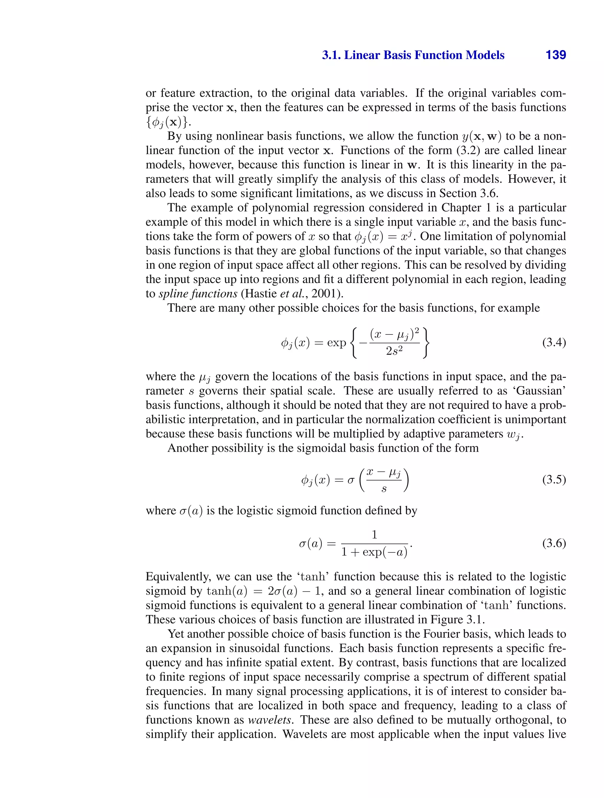
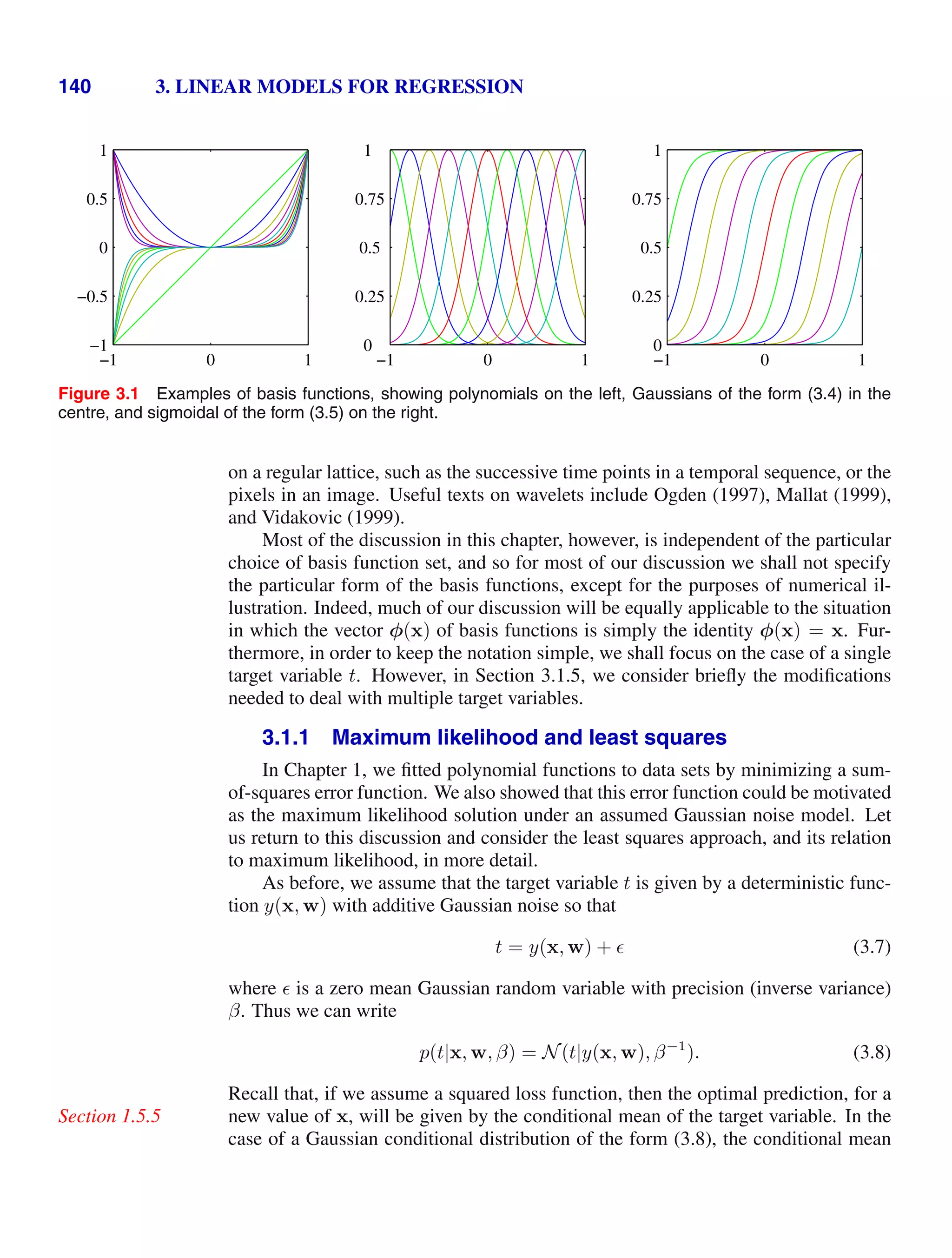
![3.1. Linear Basis Function Models 141
will be simply
E[t|x] =
tp(t|x) dt = y(x, w). (3.9)
Note that the Gaussian noise assumption implies that the conditional distribution of
t given x is unimodal, which may be inappropriate for some applications. An ex-
tension to mixtures of conditional Gaussian distributions, which permit multimodal
conditional distributions, will be discussed in Section 14.5.1.
Now consider a data set of inputs X = {x1, . . . , xN } with corresponding target
values t1, . . . , tN . We group the target variables {tn} into a column vector that we
denote by t where the typeface is chosen to distinguish it from a single observation
of a multivariate target, which would be denoted t. Making the assumption that
these data points are drawn independently from the distribution (3.8), we obtain the
following expression for the likelihood function, which is a function of the adjustable
parameters w and β, in the form
p(t|X, w, β) =
N
n=1
N(tn|wT
φ(xn), β−1
) (3.10)
where we have used (3.3). Note that in supervised learning problems such as regres-
sion (and classification), we are not seeking to model the distribution of the input
variables. Thus x will always appear in the set of conditioning variables, and so
from now on we will drop the explicit x from expressions such as p(t|x, w, β) in or-
der to keep the notation uncluttered. Taking the logarithm of the likelihood function,
and making use of the standard form (1.46) for the univariate Gaussian, we have
ln p(t|w, β) =
N
n=1
ln N(tn|wT
φ(xn), β−1
)
=
N
2
ln β −
N
2
ln(2π) − βED(w) (3.11)
where the sum-of-squares error function is defined by
ED(w) =
1
2
N
n=1
{tn − wT
φ(xn)}2
. (3.12)
Having written down the likelihood function, we can use maximum likelihood to
determine w and β. Consider first the maximization with respect to w. As observed
already in Section 1.2.5, we see that maximization of the likelihood function under a
conditional Gaussian noise distribution for a linear model is equivalent to minimizing
a sum-of-squares error function given by ED(w). The gradient of the log likelihood
function (3.11) takes the form
∇ ln p(t|w, β) =
N
n=1
tn − wT
φ(xn)
φ(xn)T
. (3.13)](https://image.slidesharecdn.com/bishop-patternrecognitionandmachinelearning-230316082240-9af1cdaa/75/Bishop-Pattern-Recognition-and-Machine-Learning-pdf-159-2048.jpg)
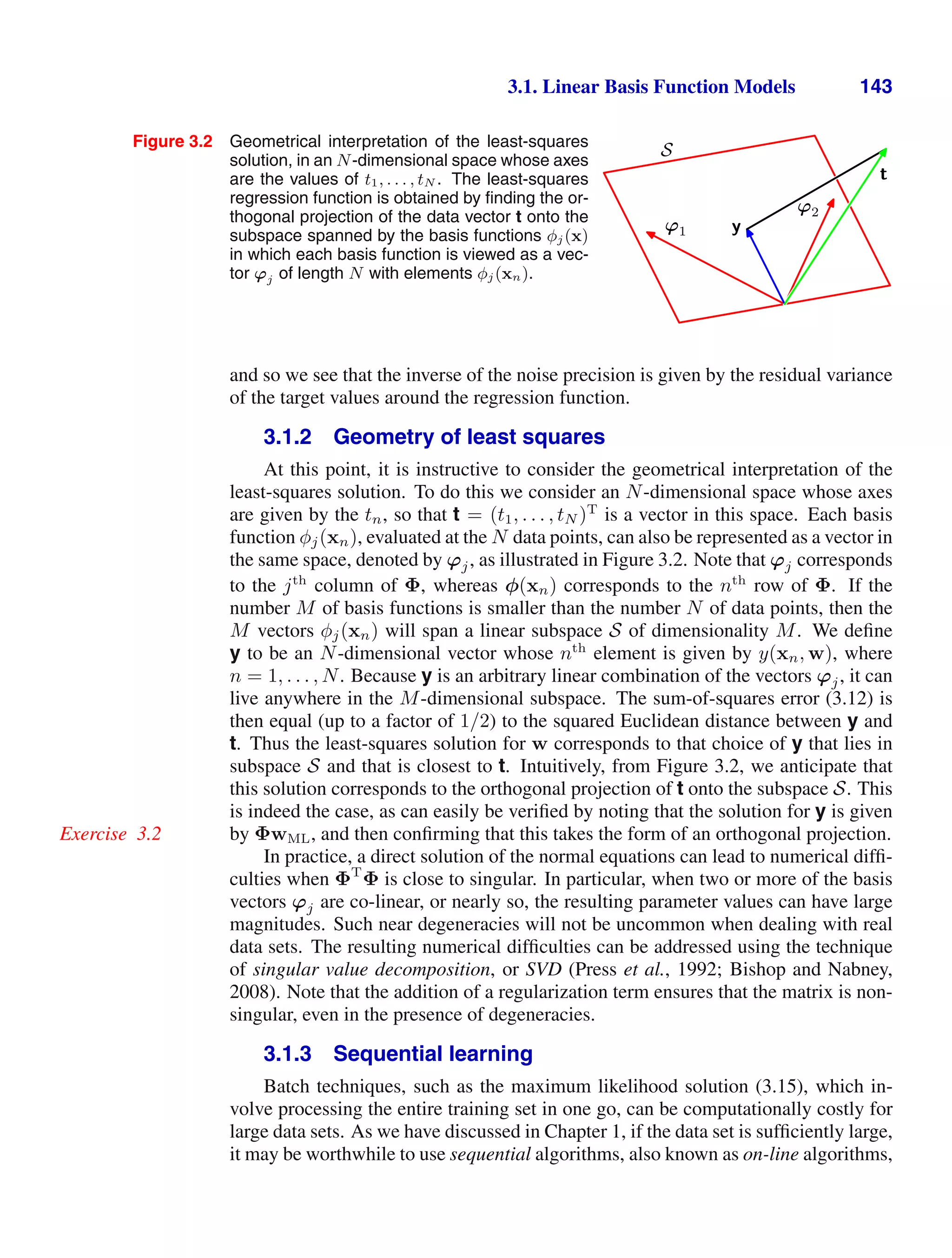
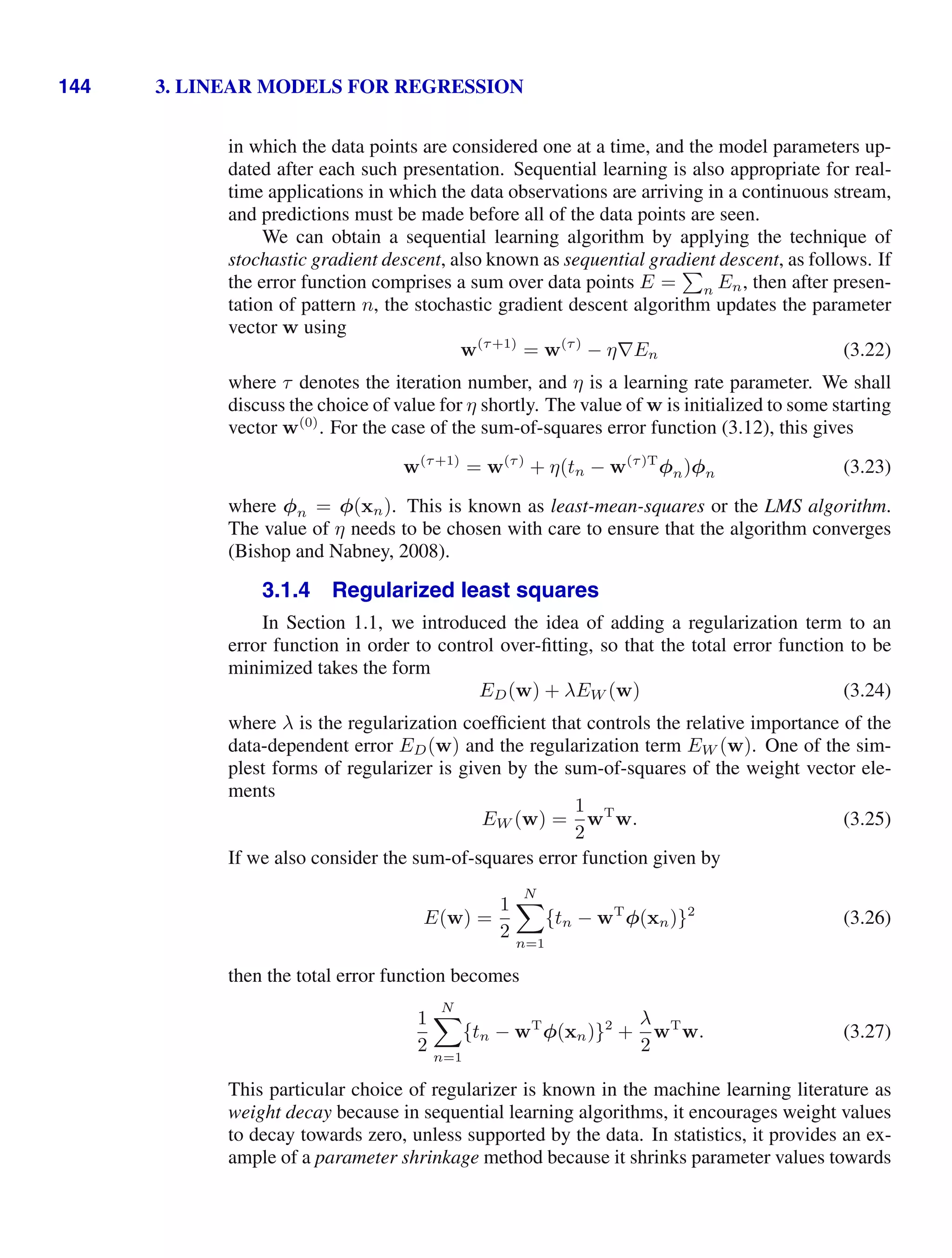
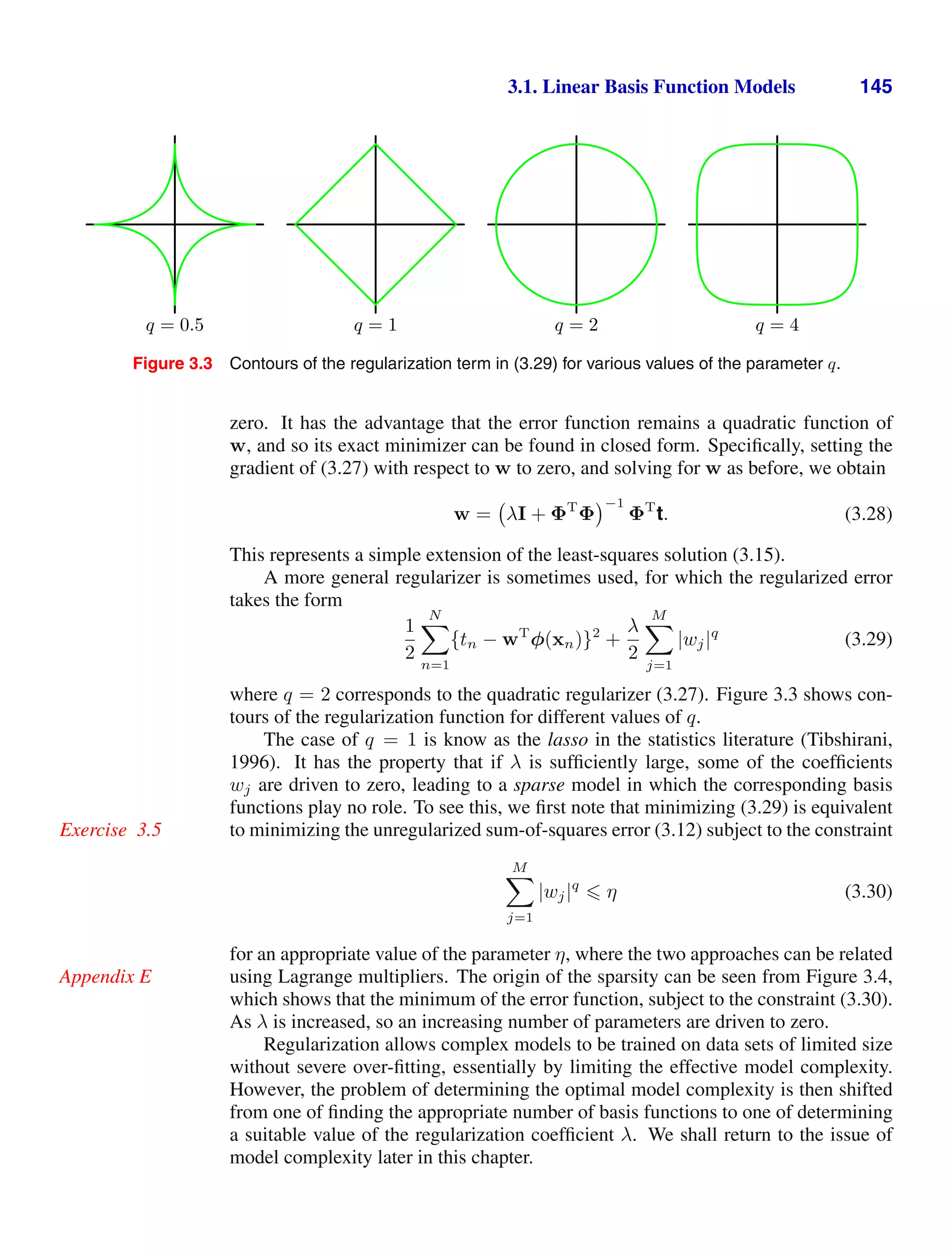
![148 3. LINEAR MODELS FOR REGRESSION
the squared loss function, for which the optimal prediction is given by the conditional
expectation, which we denote by h(x) and which is given by
h(x) = E[t|x] =
tp(t|x) dt. (3.36)
At this point, it is worth distinguishing between the squared loss function arising
from decision theory and the sum-of-squares error function that arose in the maxi-
mum likelihood estimation of model parameters. We might use more sophisticated
techniques than least squares, for example regularization or a fully Bayesian ap-
proach, to determine the conditional distribution p(t|x). These can all be combined
with the squared loss function for the purpose of making predictions.
We showed in Section 1.5.5 that the expected squared loss can be written in the
form
E[L] =
{y(x) − h(x)}
2
p(x) dx +
{h(x) − t}2
p(x, t) dx dt. (3.37)
Recall that the second term, which is independent of y(x), arises from the intrinsic
noise on the data and represents the minimum achievable value of the expected loss.
The first term depends on our choice for the function y(x), and we will seek a so-
lution for y(x) which makes this term a minimum. Because it is nonnegative, the
smallest that we can hope to make this term is zero. If we had an unlimited supply of
data (and unlimited computational resources), we could in principle find the regres-
sion function h(x) to any desired degree of accuracy, and this would represent the
optimal choice for y(x). However, in practice we have a data set D containing only
a finite number N of data points, and consequently we do not know the regression
function h(x) exactly.
If we model the h(x) using a parametric function y(x, w) governed by a pa-
rameter vector w, then from a Bayesian perspective the uncertainty in our model is
expressed through a posterior distribution over w. A frequentist treatment, however,
involves making a point estimate of w based on the data set D, and tries instead
to interpret the uncertainty of this estimate through the following thought experi-
ment. Suppose we had a large number of data sets each of size N and each drawn
independently from the distribution p(t, x). For any given data set D, we can run
our learning algorithm and obtain a prediction function y(x; D). Different data sets
from the ensemble will give different functions and consequently different values of
the squared loss. The performance of a particular learning algorithm is then assessed
by taking the average over this ensemble of data sets.
Consider the integrand of the first term in (3.37), which for a particular data set
D takes the form
{y(x; D) − h(x)}2
. (3.38)
Because this quantity will be dependent on the particular data set D, we take its aver-
age over the ensemble of data sets. If we add and subtract the quantity ED[y(x; D)]](https://image.slidesharecdn.com/bishop-patternrecognitionandmachinelearning-230316082240-9af1cdaa/75/Bishop-Pattern-Recognition-and-Machine-Learning-pdf-166-2048.jpg)
![3.2. The Bias-Variance Decomposition 149
inside the braces, and then expand, we obtain
{y(x; D) − ED[y(x; D)] + ED[y(x; D)] − h(x)}2
= {y(x; D) − ED[y(x; D)]}2
+ {ED[y(x; D)] − h(x)}2
+2{y(x; D) − ED[y(x; D)]}{ED[y(x; D)] − h(x)}. (3.39)
We now take the expectation of this expression with respect to D and note that the
final term will vanish, giving
ED
{y(x; D) − h(x)}2
= {ED[y(x; D)] − h(x)}2
( )* +
(bias)2
+ ED
{y(x; D) − ED[y(x; D)]}2
( )* +
variance
. (3.40)
We see that the expected squared difference between y(x; D) and the regression
function h(x) can be expressed as the sum of two terms. The first term, called the
squared bias, represents the extent to which the average prediction over all data sets
differs from the desired regression function. The second term, called the variance,
measures the extent to which the solutions for individual data sets vary around their
average, and hence this measures the extent to which the function y(x; D) is sensitive
to the particular choice of data set. We shall provide some intuition to support these
definitions shortly when we consider a simple example.
So far, we have considered a single input value x. If we substitute this expansion
back into (3.37), we obtain the following decomposition of the expected squared loss
expected loss = (bias)2
+ variance + noise (3.41)
where
(bias)2
=
{ED[y(x; D)] − h(x)}2
p(x) dx (3.42)
variance =
ED
{y(x; D) − ED[y(x; D)]}2
p(x) dx (3.43)
noise =
{h(x) − t}2
p(x, t) dx dt (3.44)
and the bias and variance terms now refer to integrated quantities.
Our goal is to minimize the expected loss, which we have decomposed into the
sum of a (squared) bias, a variance, and a constant noise term. As we shall see, there
is a trade-off between bias and variance, with very flexible models having low bias
and high variance, and relatively rigid models having high bias and low variance.
The model with the optimal predictive capability is the one that leads to the best
balance between bias and variance. This is illustrated by considering the sinusoidal
data set from Chapter 1. Here we generate 100 data sets, each containing N = 25
Appendix A
data points, independently from the sinusoidal curve h(x) = sin(2πx). The data
sets are indexed by l = 1, . . . , L, where L = 100, and for each data set D(l)
we](https://image.slidesharecdn.com/bishop-patternrecognitionandmachinelearning-230316082240-9af1cdaa/75/Bishop-Pattern-Recognition-and-Machine-Learning-pdf-167-2048.jpg)
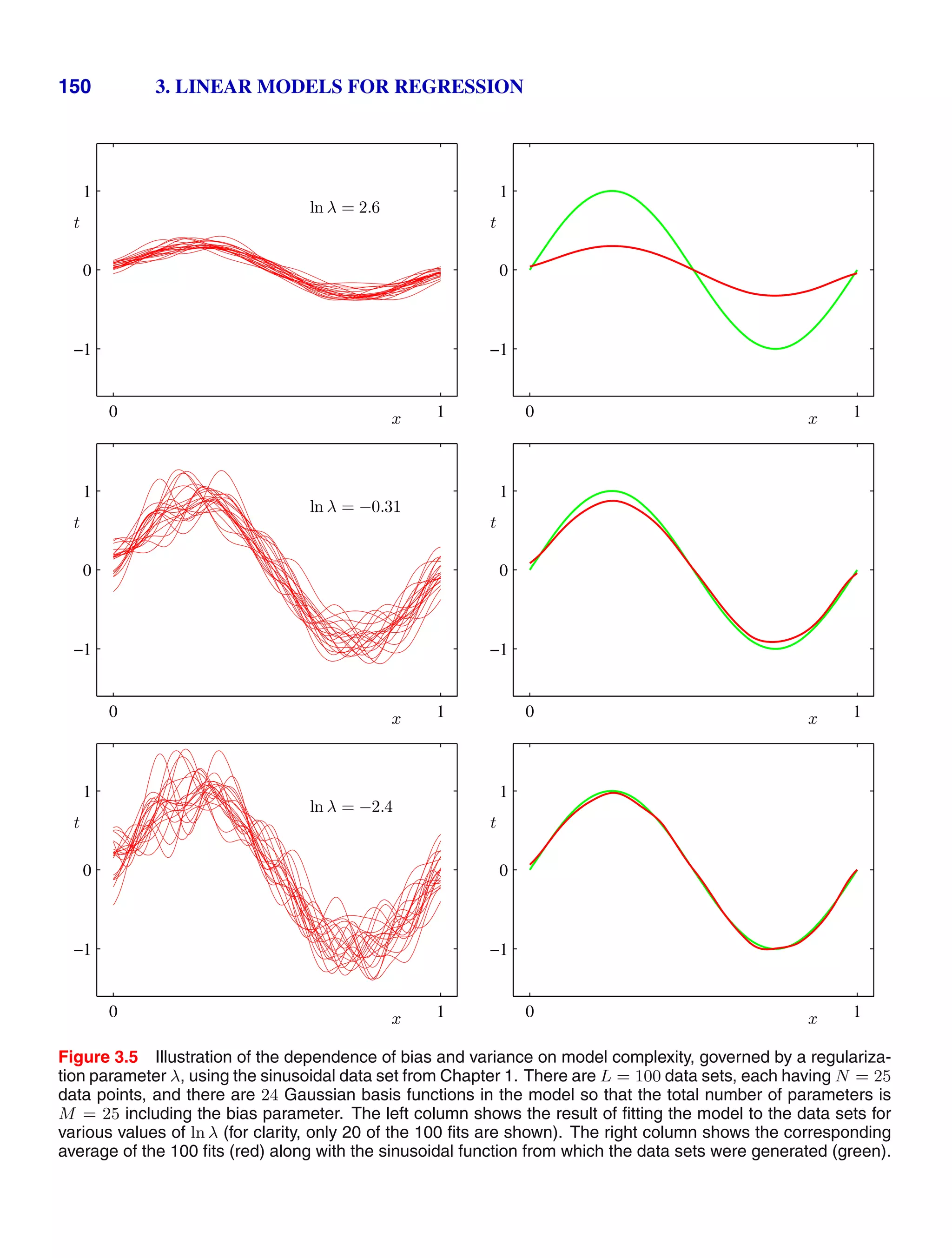
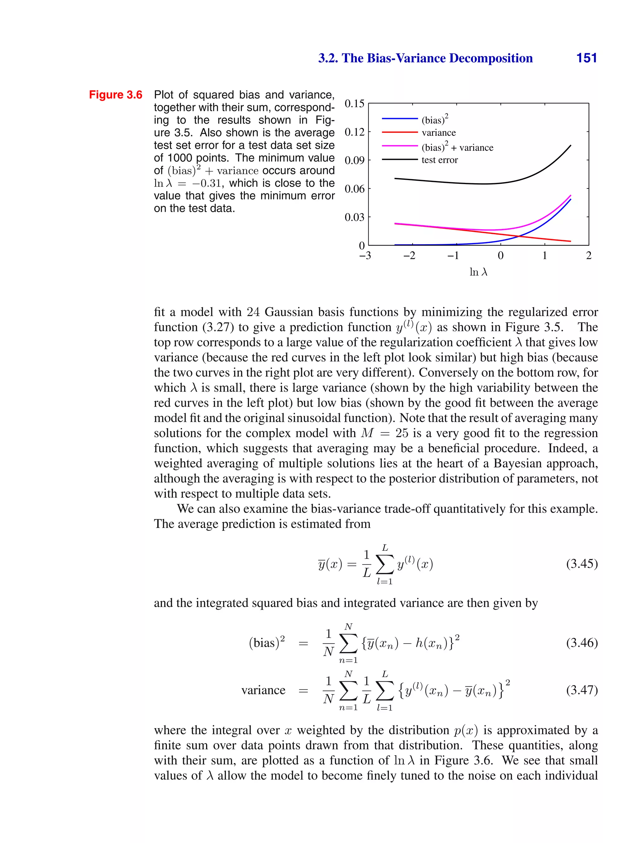
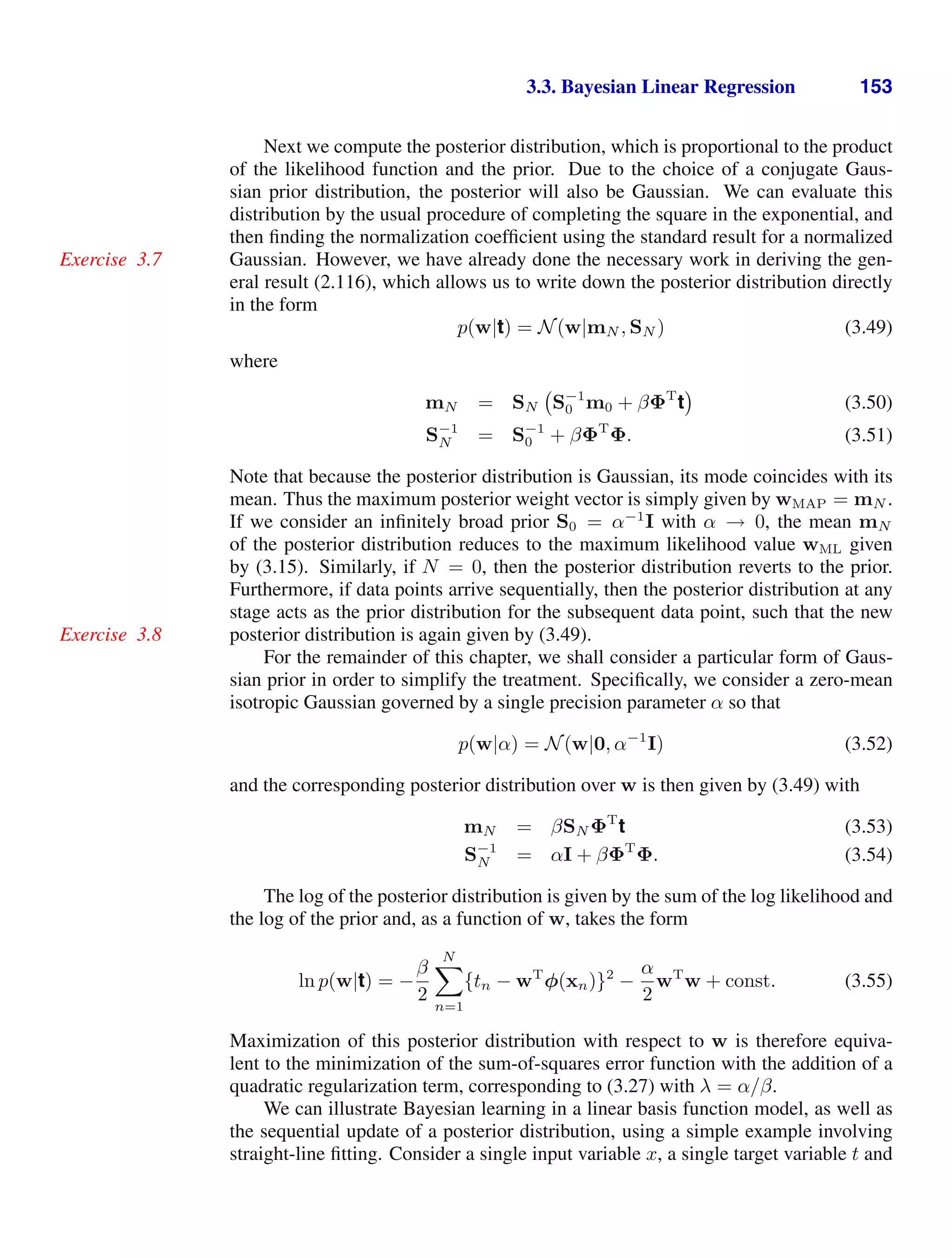
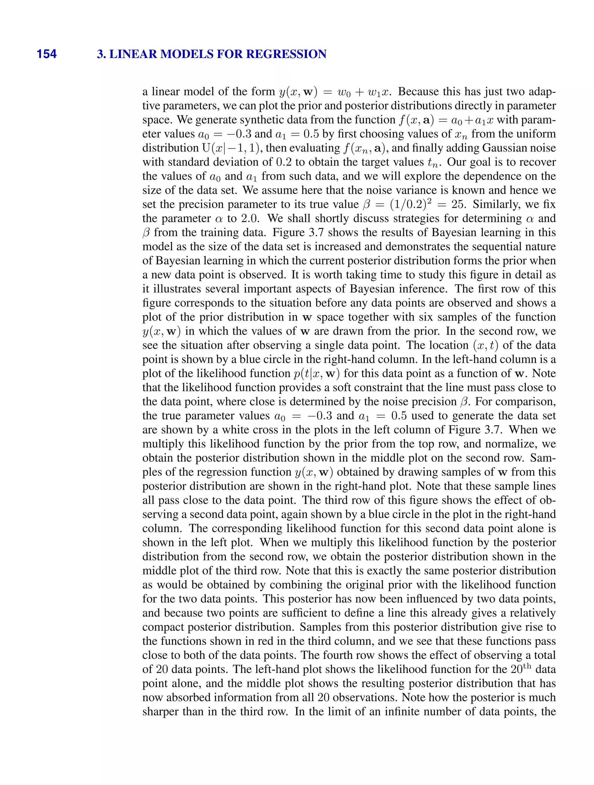
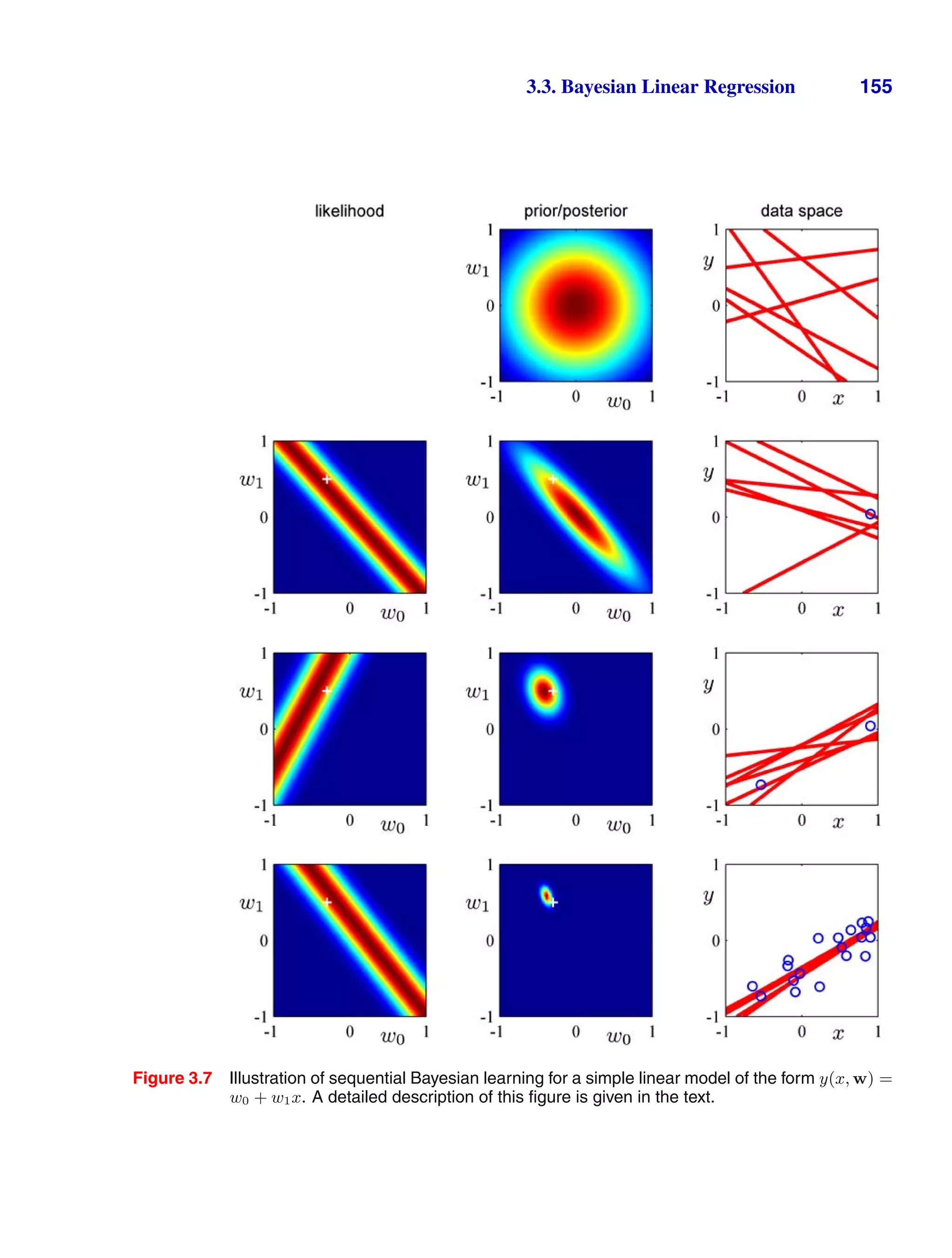
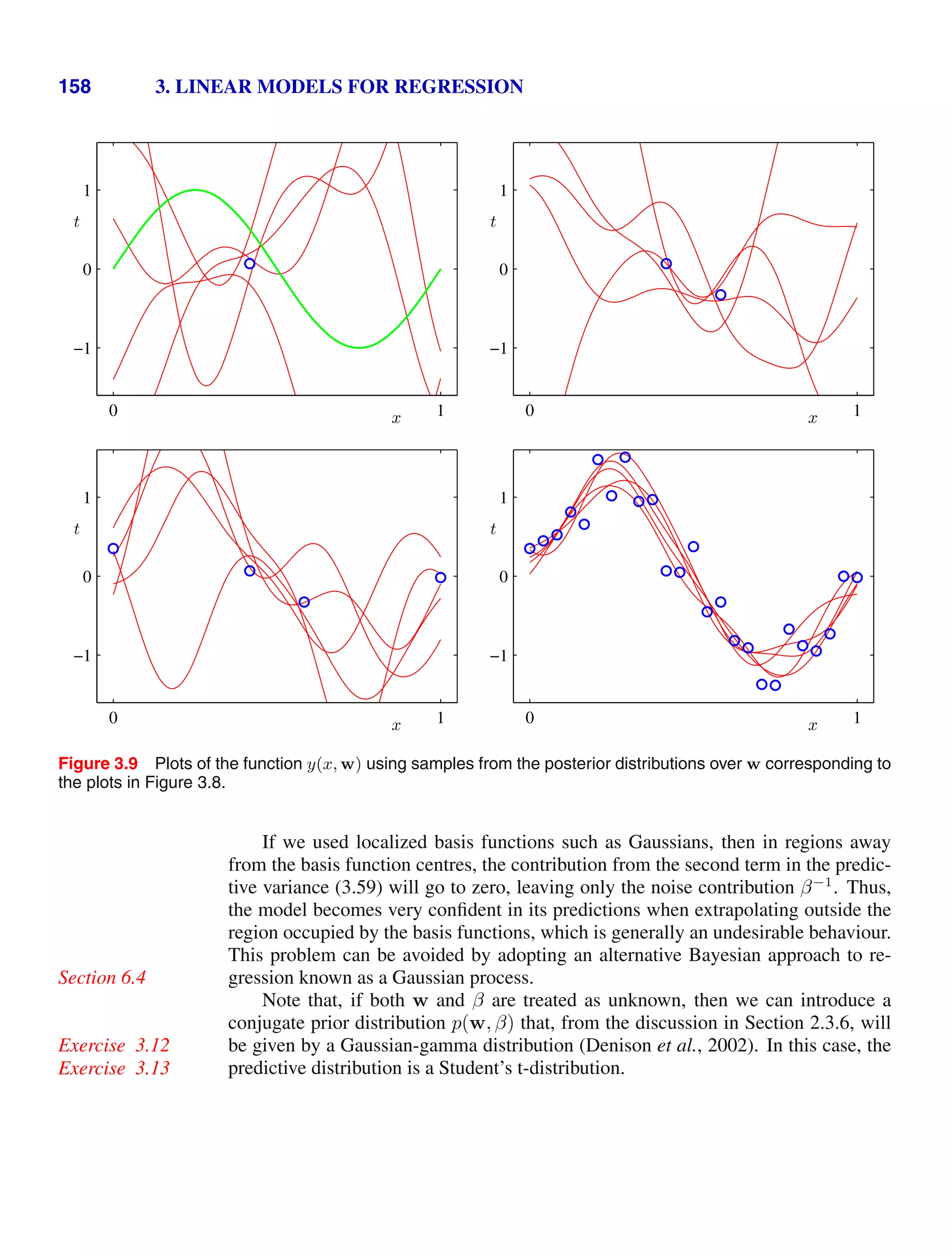
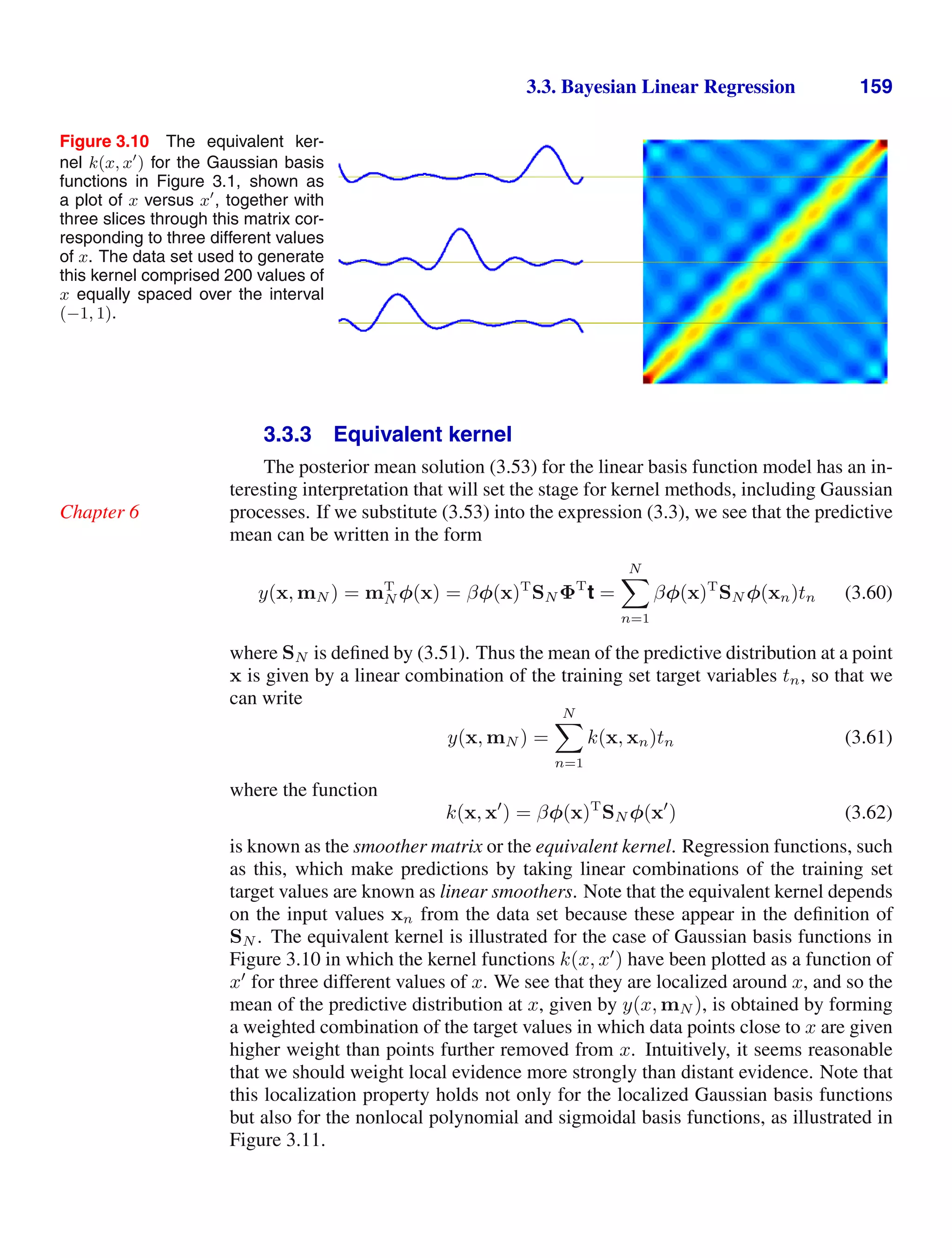
![160 3. LINEAR MODELS FOR REGRESSION
Figure 3.11 Examples of equiva-
lent kernels k(x, x
) for x = 0
plotted as a function of x
, corre-
sponding (left) to the polynomial ba-
sis functions and (right) to the sig-
moidal basis functions shown in Fig-
ure 3.1. Note that these are local-
ized functions of x
even though the
corresponding basis functions are
nonlocal. −1 0 1
0
0.02
0.04
−1 0 1
0
0.02
0.04
Further insight into the role of the equivalent kernel can be obtained by consid-
ering the covariance between y(x) and y(x
), which is given by
cov[y(x), y(x
)] = cov[φ(x)T
w, wT
φ(x
)]
= φ(x)T
SN φ(x
) = β−1
k(x, x
) (3.63)
where we have made use of (3.49) and (3.62). From the form of the equivalent
kernel, we see that the predictive mean at nearby points will be highly correlated,
whereas for more distant pairs of points the correlation will be smaller.
The predictive distribution shown in Figure 3.8 allows us to visualize the point-
wise uncertainty in the predictions, governed by (3.59). However, by drawing sam-
ples from the posterior distribution over w, and plotting the corresponding model
functions y(x, w) as in Figure 3.9, we are visualizing the joint uncertainty in the
posterior distribution between the y values at two (or more) x values, as governed by
the equivalent kernel.
The formulation of linear regression in terms of a kernel function suggests an
alternative approach to regression as follows. Instead of introducing a set of basis
functions, which implicitly determines an equivalent kernel, we can instead define
a localized kernel directly and use this to make predictions for new input vectors x,
given the observed training set. This leads to a practical framework for regression
(and classification) called Gaussian processes, which will be discussed in detail in
Section 6.4.
We have seen that the effective kernel defines the weights by which the training
set target values are combined in order to make a prediction at a new value of x, and
it can be shown that these weights sum to one, in other words
N
n=1
k(x, xn) = 1 (3.64)
for all values of x. This intuitively pleasing result can easily be proven informally
Exercise 3.14
by noting that the summation is equivalent to considering the predictive mean
y(x)
for a set of target data in which tn = 1 for all n. Provided the basis functions are
linearly independent, that there are more data points than basis functions, and that
one of the basis functions is constant (corresponding to the bias parameter), then it is
clear that we can fit the training data exactly and hence that the predictive mean will](https://image.slidesharecdn.com/bishop-patternrecognitionandmachinelearning-230316082240-9af1cdaa/75/Bishop-Pattern-Recognition-and-Machine-Learning-pdf-178-2048.jpg)
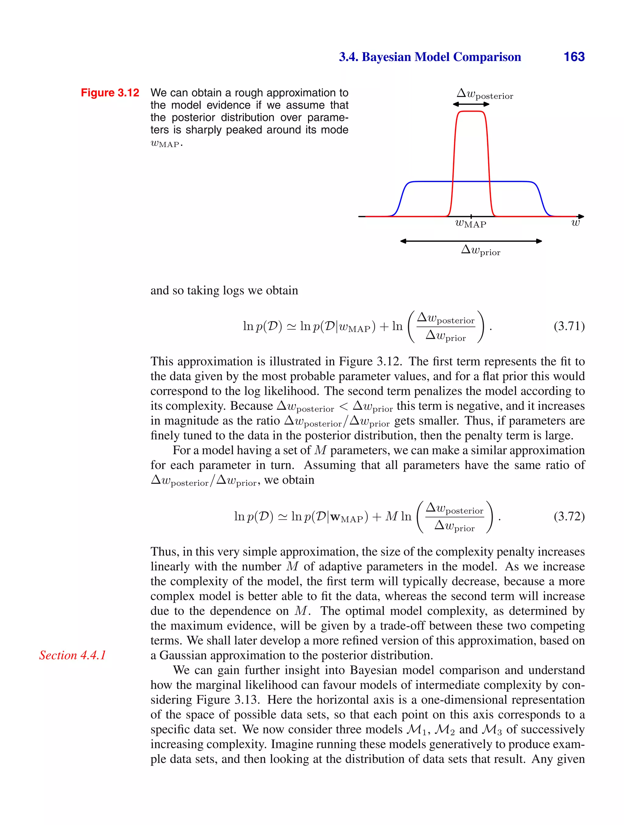
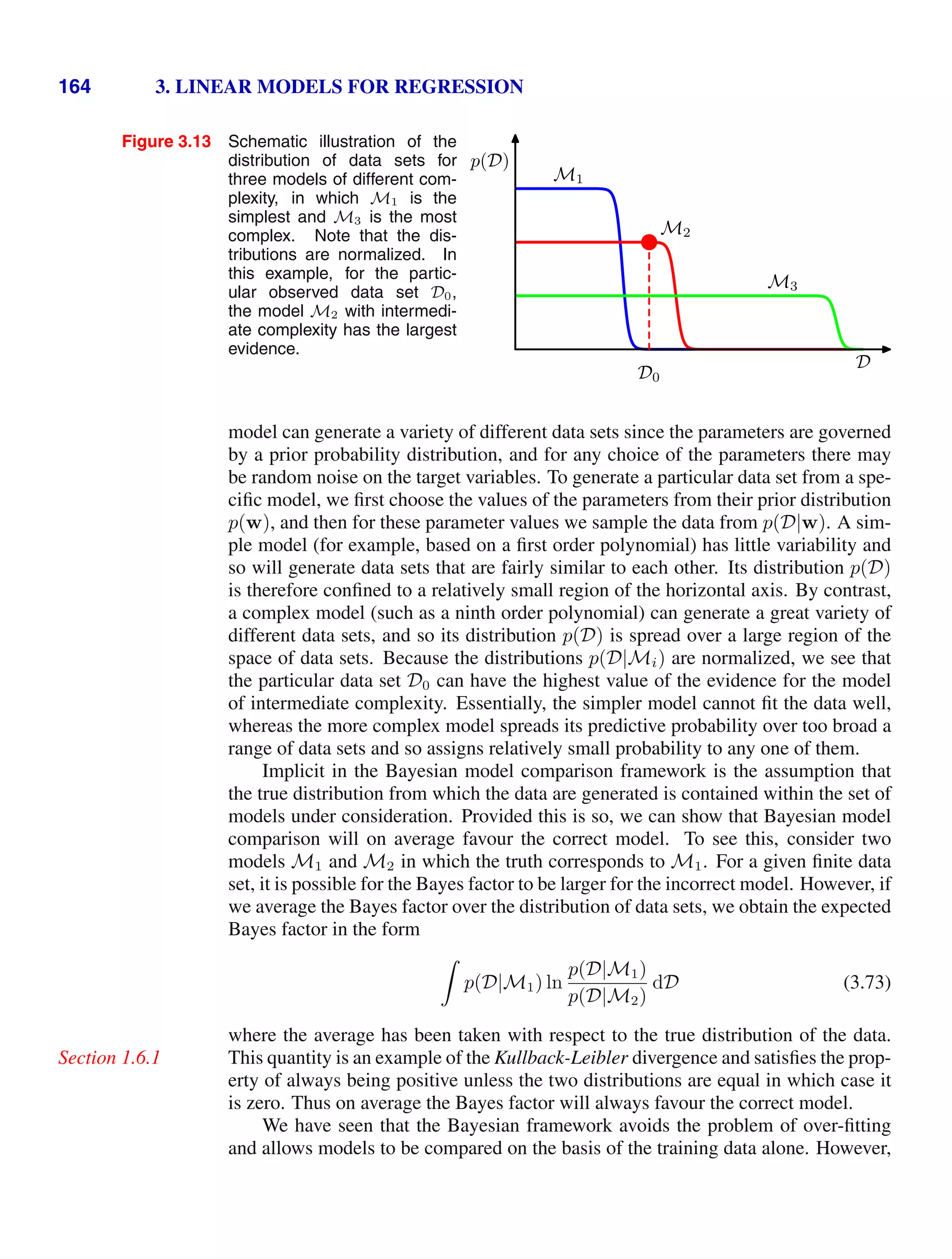
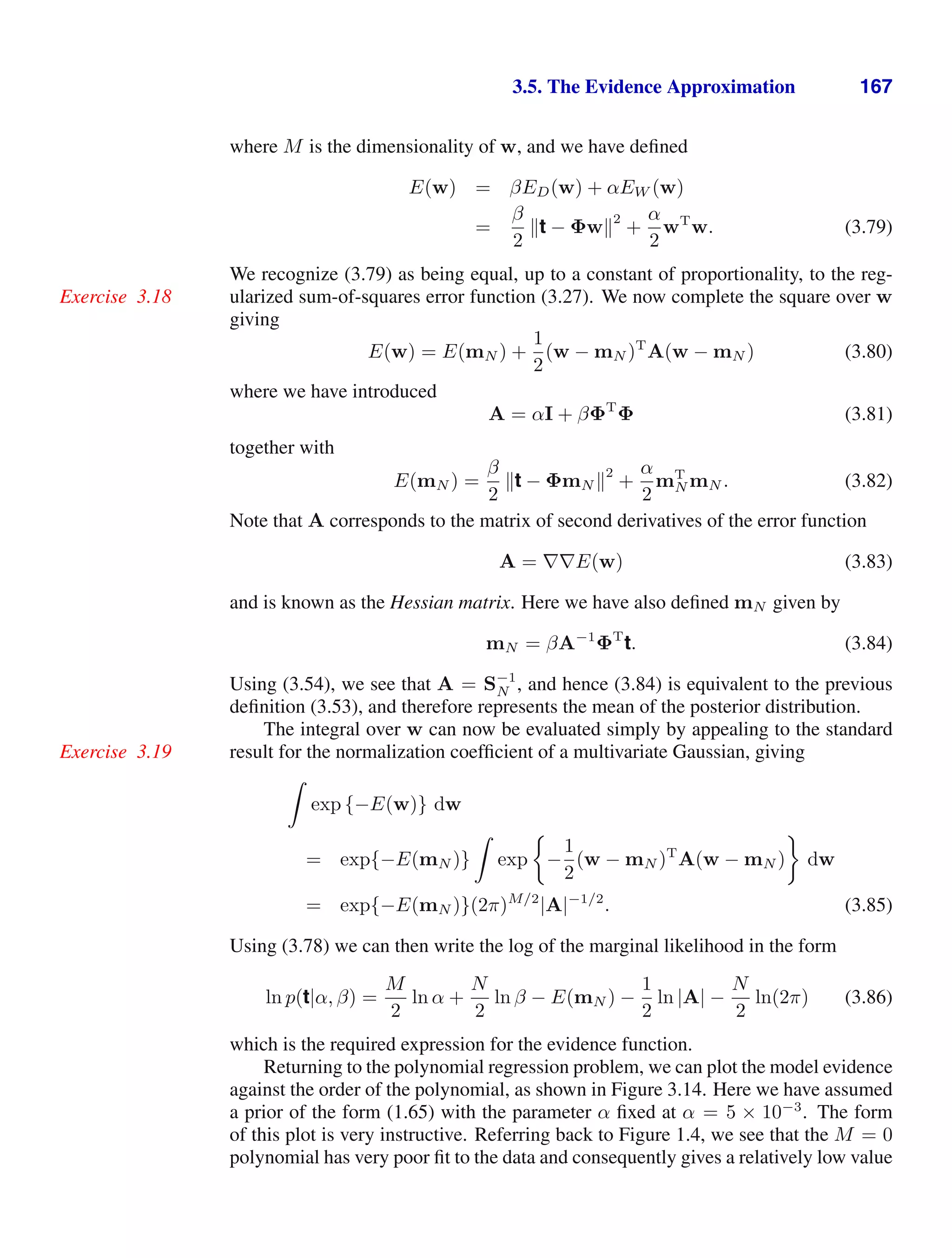
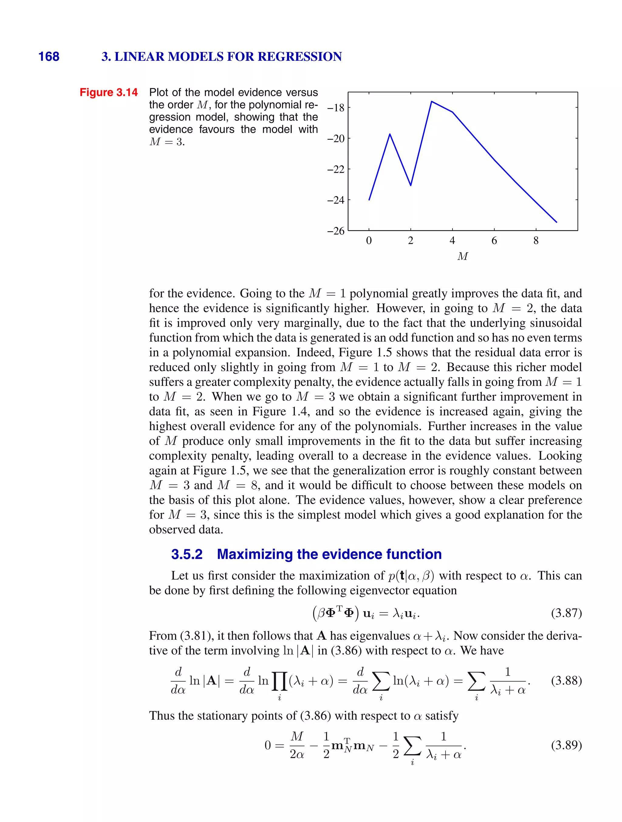
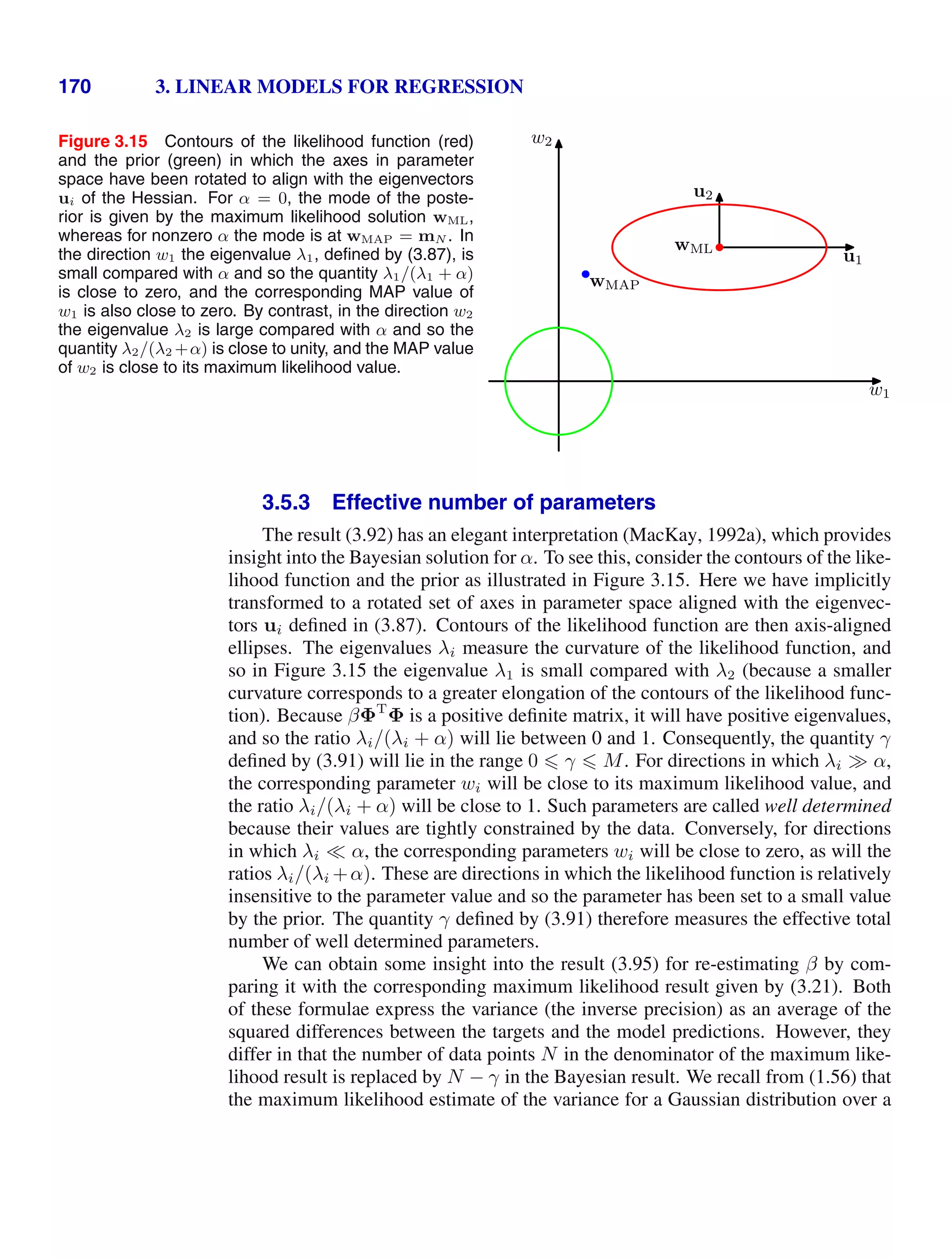
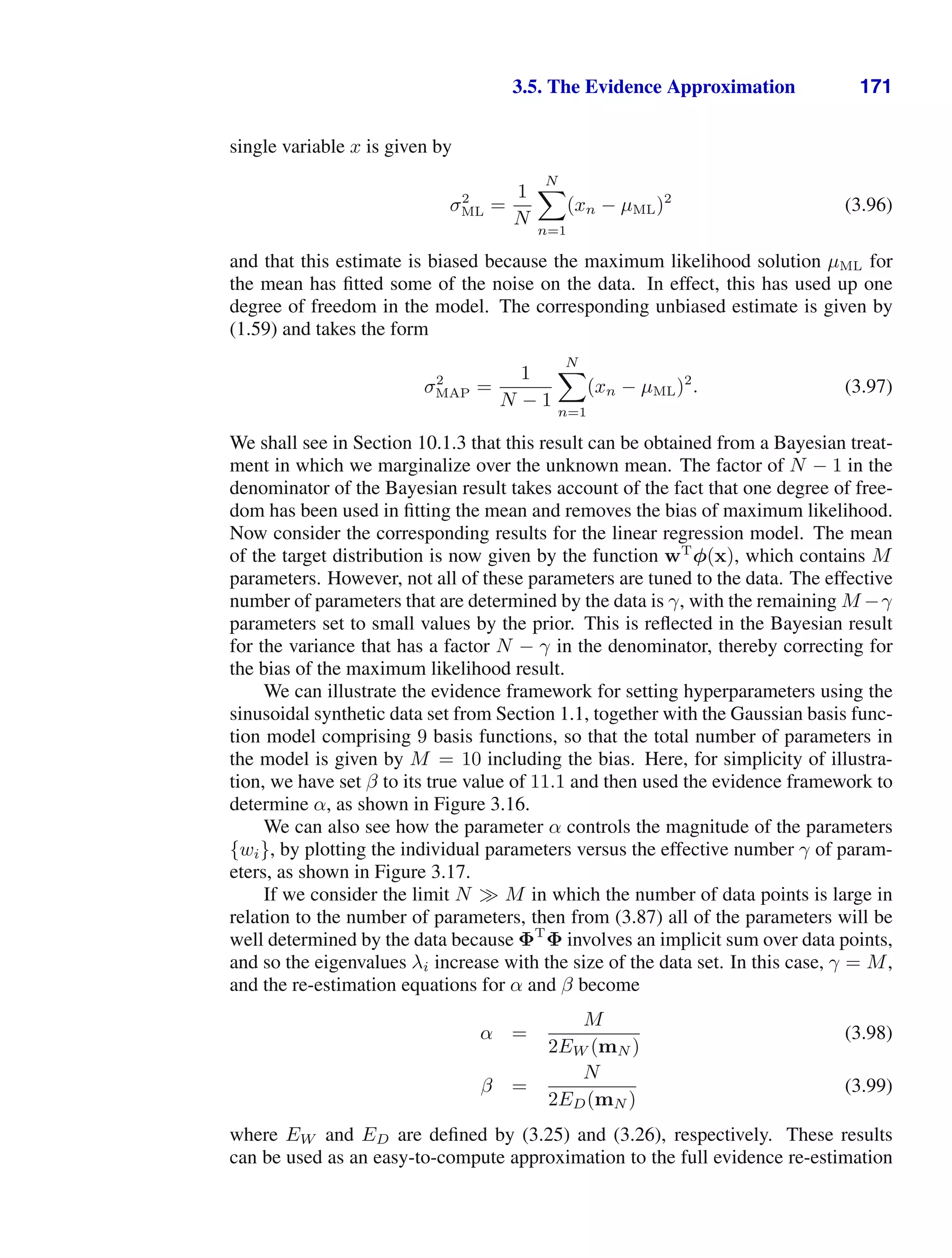
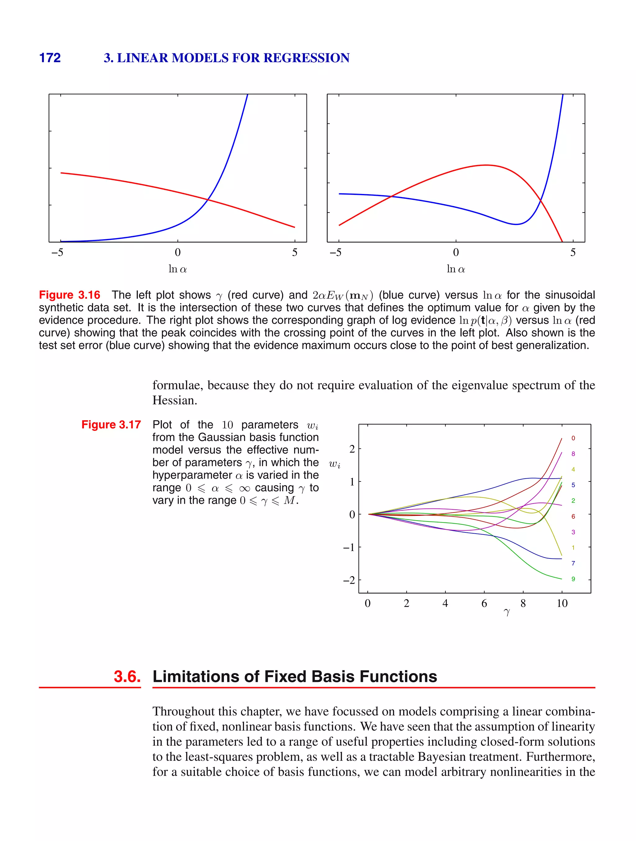
![174 3. LINEAR MODELS FOR REGRESSION
3.2 ( ) Show that the matrix
Φ(ΦT
Φ)−1
ΦT
(3.103)
takes any vector v and projects it onto the space spanned by the columns of Φ. Use
this result to show that the least-squares solution (3.15) corresponds to an orthogonal
projection of the vector t onto the manifold S as shown in Figure 3.2.
3.3 ( ) Consider a data set in which each data point tn is associated with a weighting
factor rn 0, so that the sum-of-squares error function becomes
ED(w) =
1
2
N
n=1
rn
tn − wT
φ(xn)
2
. (3.104)
Find an expression for the solution w
that minimizes this error function. Give two
alternative interpretations of the weighted sum-of-squares error function in terms of
(i) data dependent noise variance and (ii) replicated data points.
3.4 ( ) www Consider a linear model of the form
y(x, w) = w0 +
D
i=1
wixi (3.105)
together with a sum-of-squares error function of the form
ED(w) =
1
2
N
n=1
{y(xn, w) − tn}
2
. (3.106)
Now suppose that Gaussian noise i with zero mean and variance σ2
is added in-
dependently to each of the input variables xi. By making use of E[i] = 0 and
E[ij] = δijσ2
, show that minimizing ED averaged over the noise distribution is
equivalent to minimizing the sum-of-squares error for noise-free input variables with
the addition of a weight-decay regularization term, in which the bias parameter w0
is omitted from the regularizer.
3.5 ( ) www Using the technique of Lagrange multipliers, discussed in Appendix E,
show that minimization of the regularized error function (3.29) is equivalent to mini-
mizing the unregularized sum-of-squares error (3.12) subject to the constraint (3.30).
Discuss the relationship between the parameters η and λ.
3.6 ( ) www Consider a linear basis function regression model for a multivariate
target variable t having a Gaussian distribution of the form
p(t|W, Σ) = N(t|y(x, W), Σ) (3.107)
where
y(x, W) = WT
φ(x) (3.108)](https://image.slidesharecdn.com/bishop-patternrecognitionandmachinelearning-230316082240-9af1cdaa/75/Bishop-Pattern-Recognition-and-Machine-Learning-pdf-192-2048.jpg)
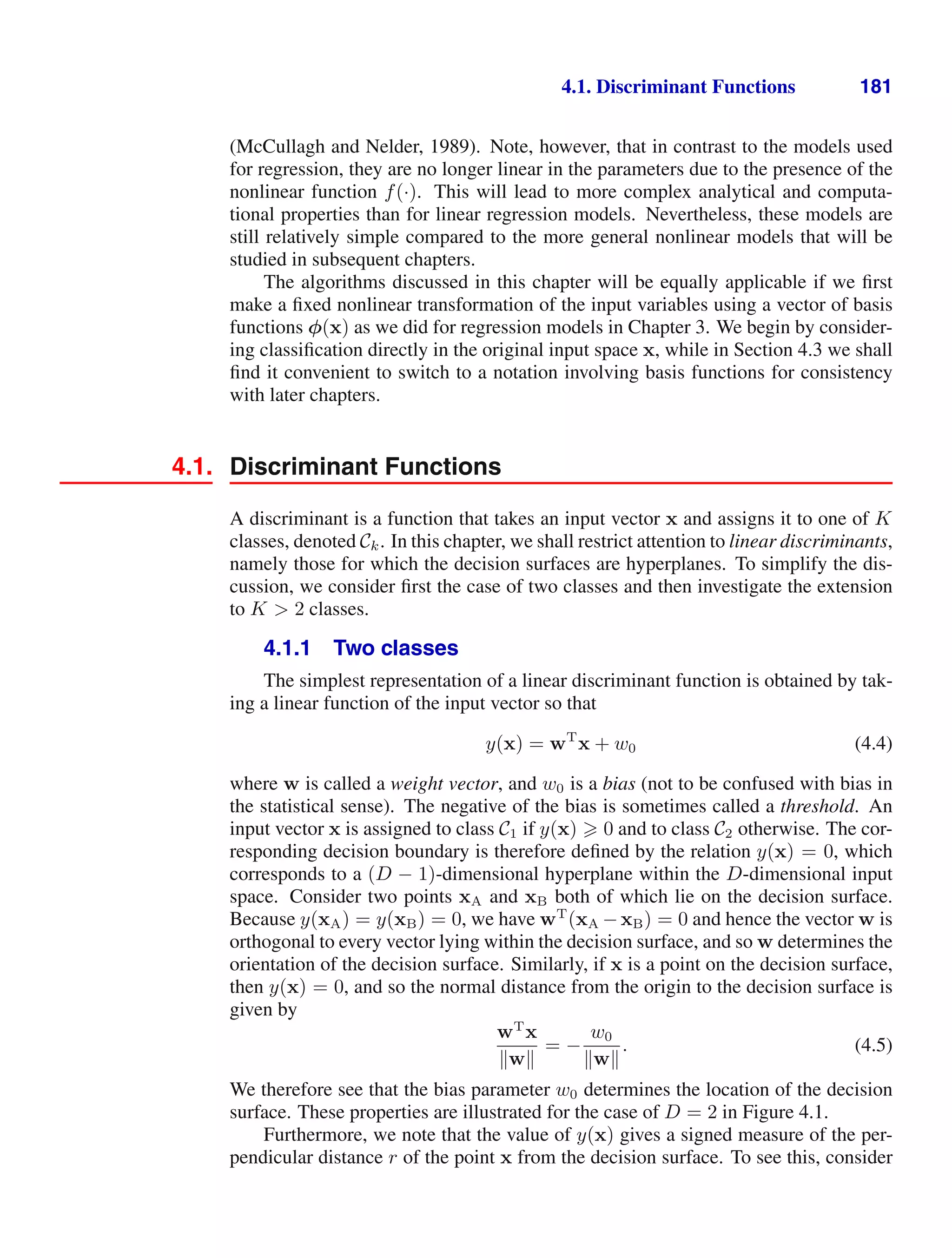
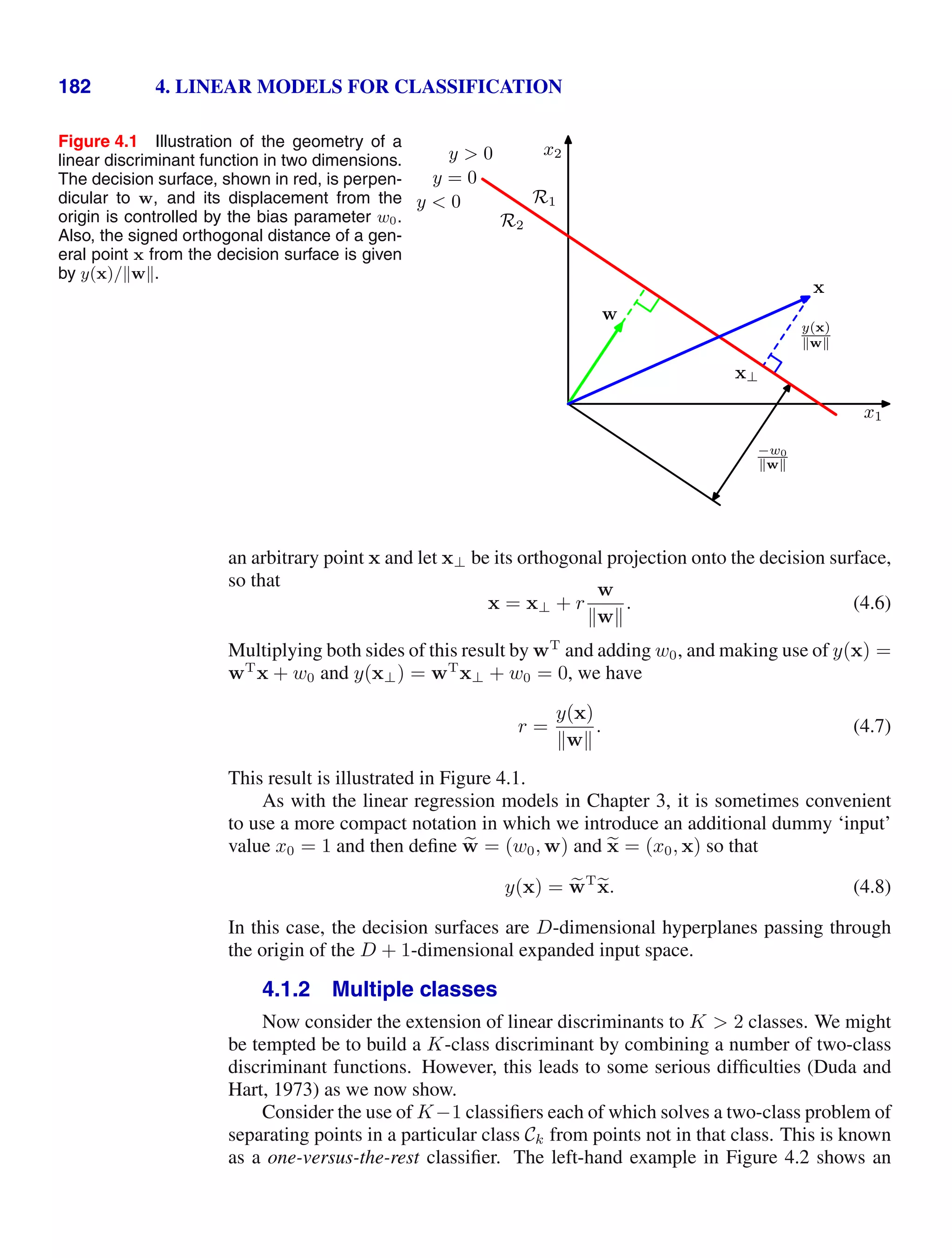
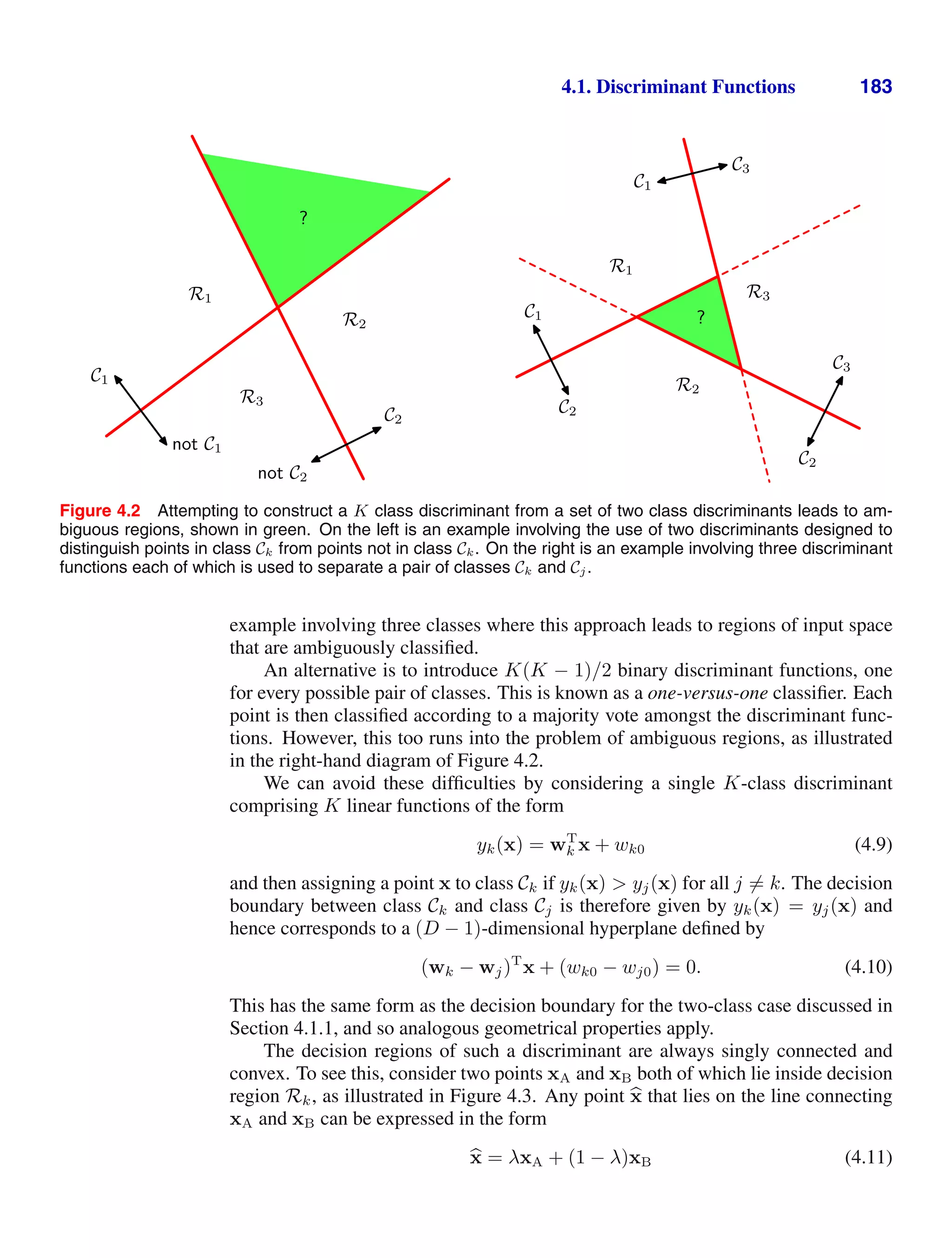
![184 4. LINEAR MODELS FOR CLASSIFICATION
Figure 4.3 Illustration of the decision regions for a mul-
ticlass linear discriminant, with the decision
boundaries shown in red. If two points xA
and xB both lie inside the same decision re-
gion Rk, then any point b
x that lies on the line
connecting these two points must also lie in
Rk, and hence the decision region must be
singly connected and convex.
Ri
Rj
Rk
xA
xB
x̂
where 0 λ 1. From the linearity of the discriminant functions, it follows that
yk(
x) = λyk(xA) + (1 − λ)yk(xB). (4.12)
Because both xA and xB lie inside Rk, it follows that yk(xA) yj(xA), and
yk(xB) yj(xB), for all j = k, and hence yk(
x) yj(
x), and so
x also lies
inside Rk. Thus Rk is singly connected and convex.
Note that for two classes, we can either employ the formalism discussed here,
based on two discriminant functions y1(x) and y2(x), or else use the simpler but
equivalent formulation described in Section 4.1.1 based on a single discriminant
function y(x).
We now explore three approaches to learning the parameters of linear discrimi-
nant functions, based on least squares, Fisher’s linear discriminant, and the percep-
tron algorithm.
4.1.3 Least squares for classification
In Chapter 3, we considered models that were linear functions of the parame-
ters, and we saw that the minimization of a sum-of-squares error function led to a
simple closed-form solution for the parameter values. It is therefore tempting to see
if we can apply the same formalism to classification problems. Consider a general
classification problem with K classes, with a 1-of-K binary coding scheme for the
target vector t. One justification for using least squares in such a context is that it
approximates the conditional expectation E[t|x] of the target values given the input
vector. For the binary coding scheme, this conditional expectation is given by the
vector of posterior class probabilities. Unfortunately, however, these probabilities
are typically approximated rather poorly, indeed the approximations can have values
outside the range (0, 1), due to the limited flexibility of a linear model as we shall
see shortly.
Each class Ck is described by its own linear model so that
yk(x) = wT
k x + wk0 (4.13)
where k = 1, . . . , K. We can conveniently group these together using vector nota-
tion so that
y(x) = ,
WT
x (4.14)](https://image.slidesharecdn.com/bishop-patternrecognitionandmachinelearning-230316082240-9af1cdaa/75/Bishop-Pattern-Recognition-and-Machine-Learning-pdf-201-2048.jpg)
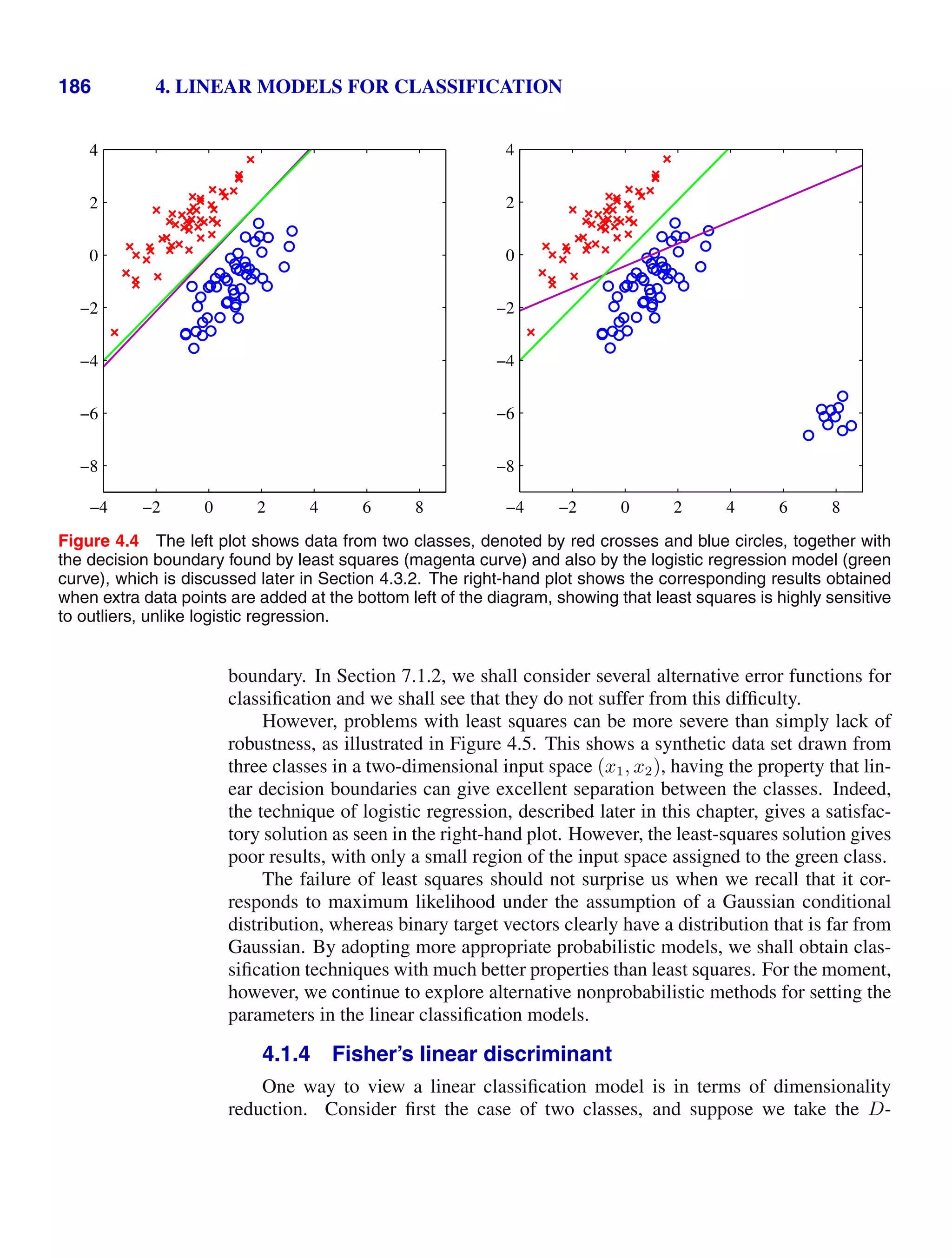
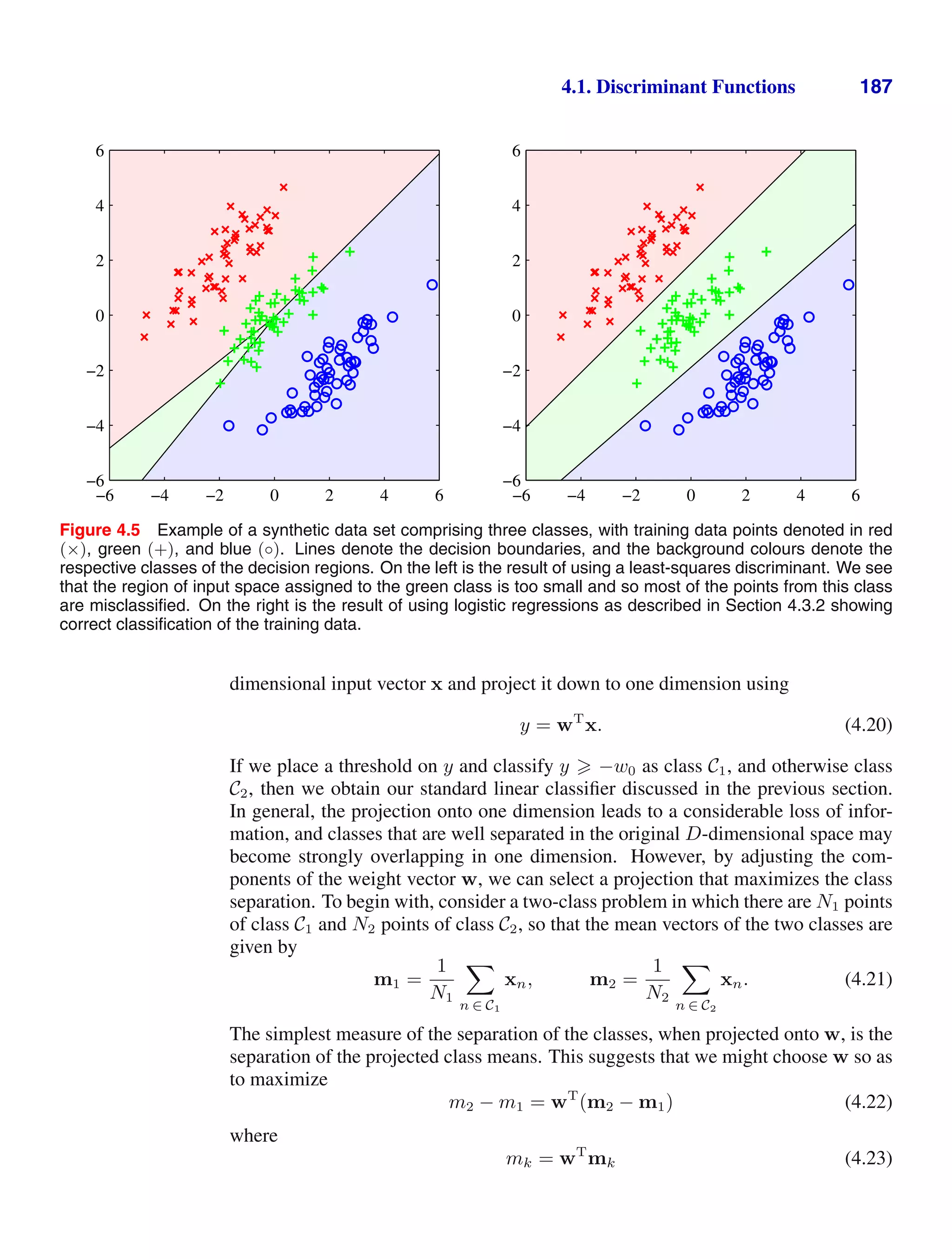
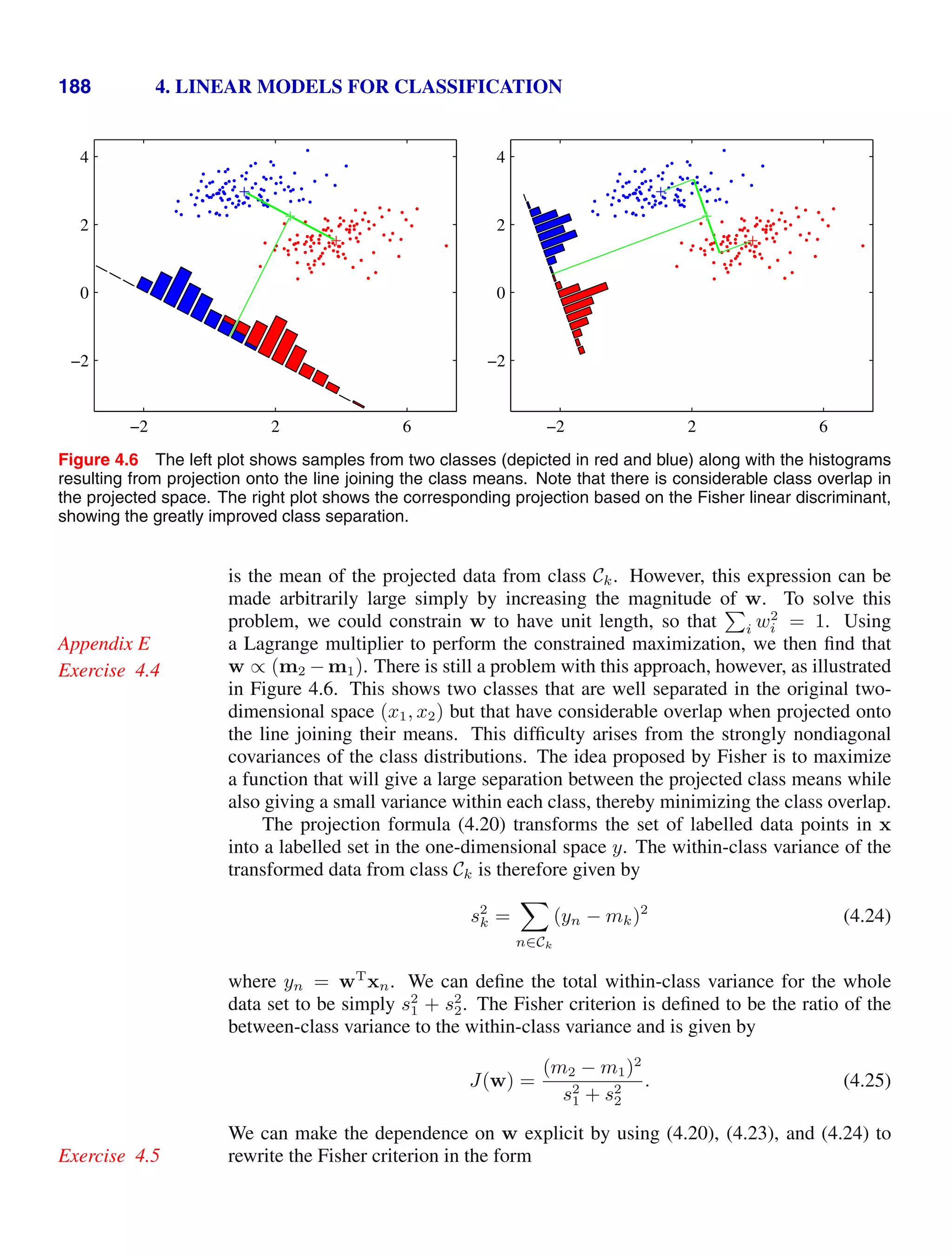
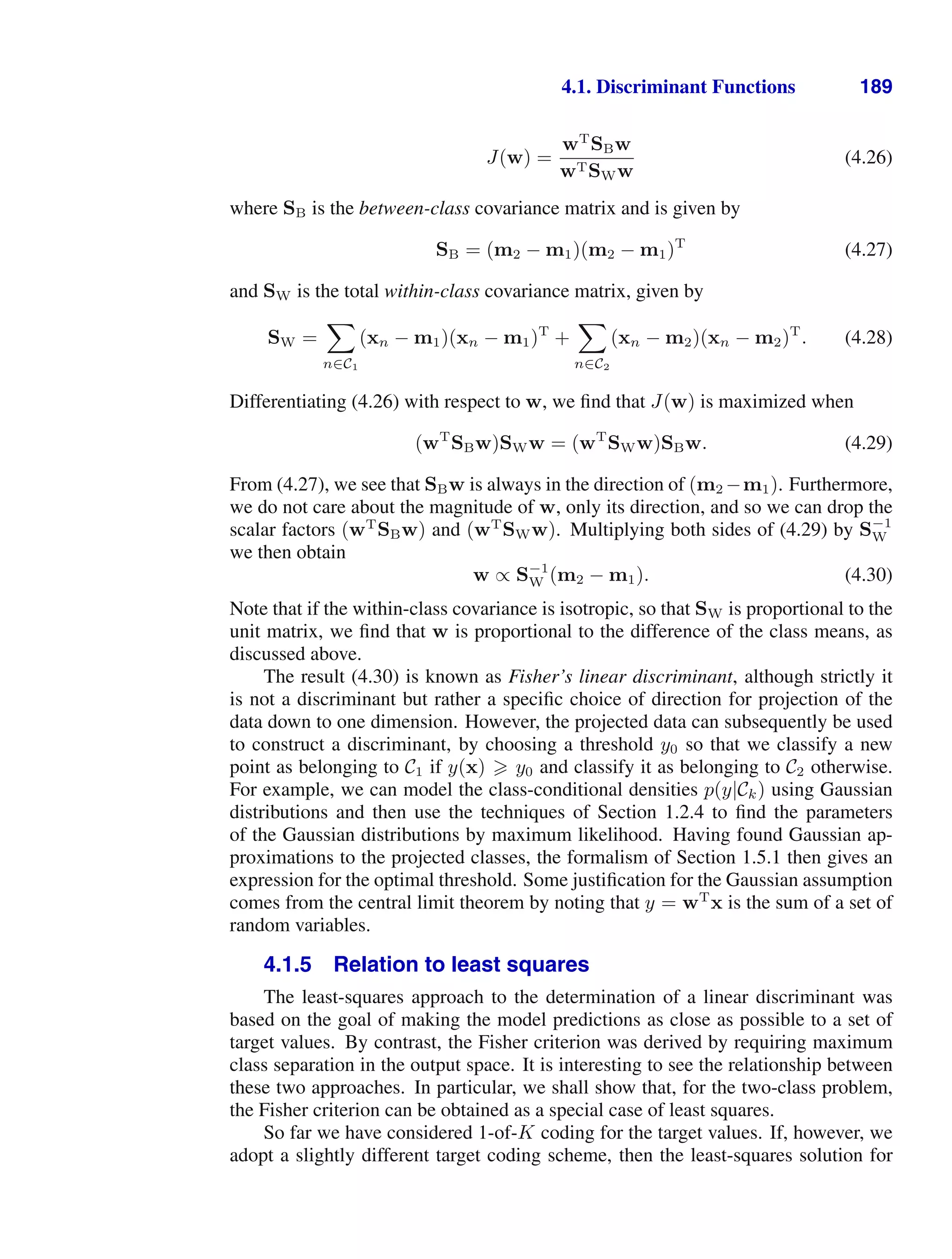
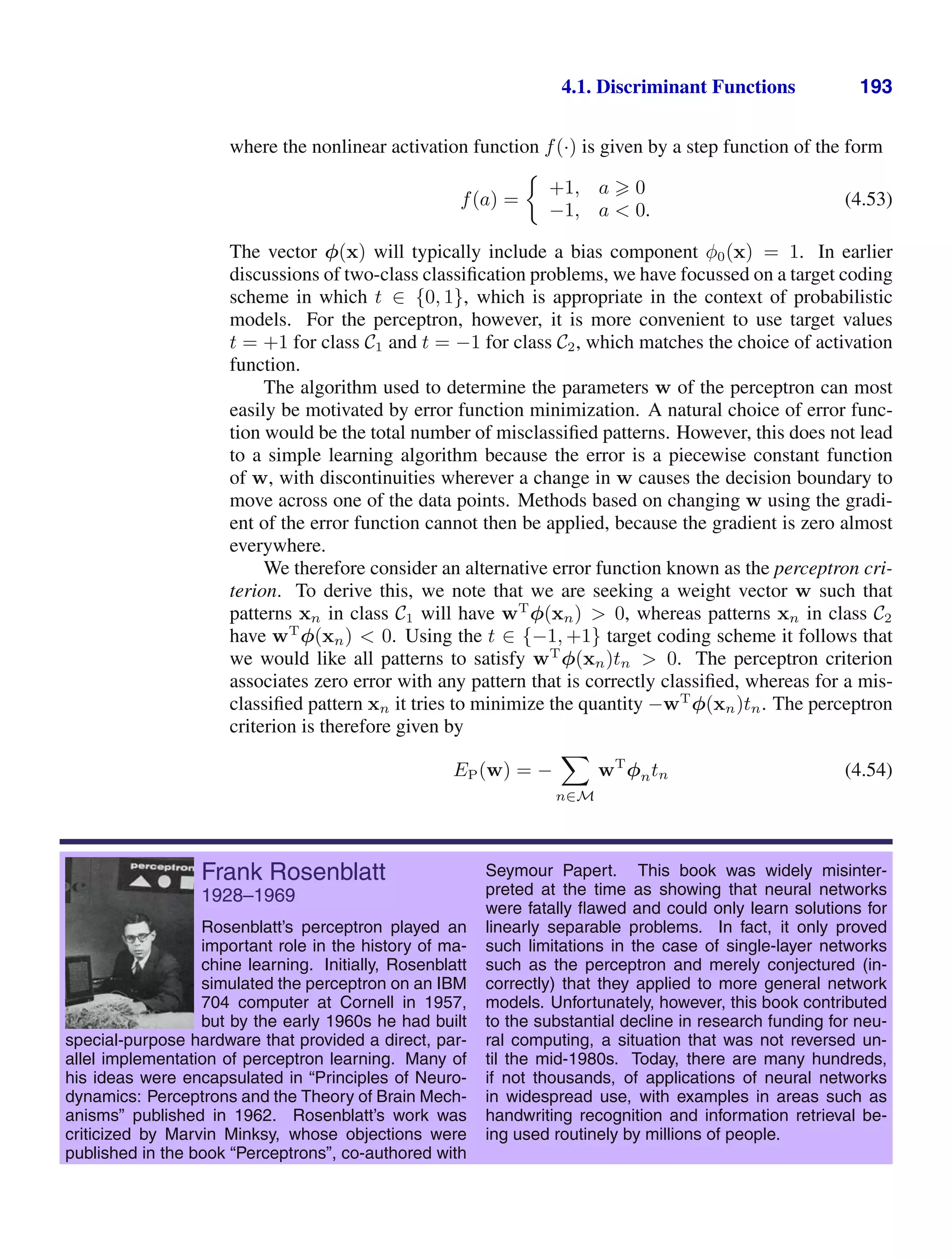
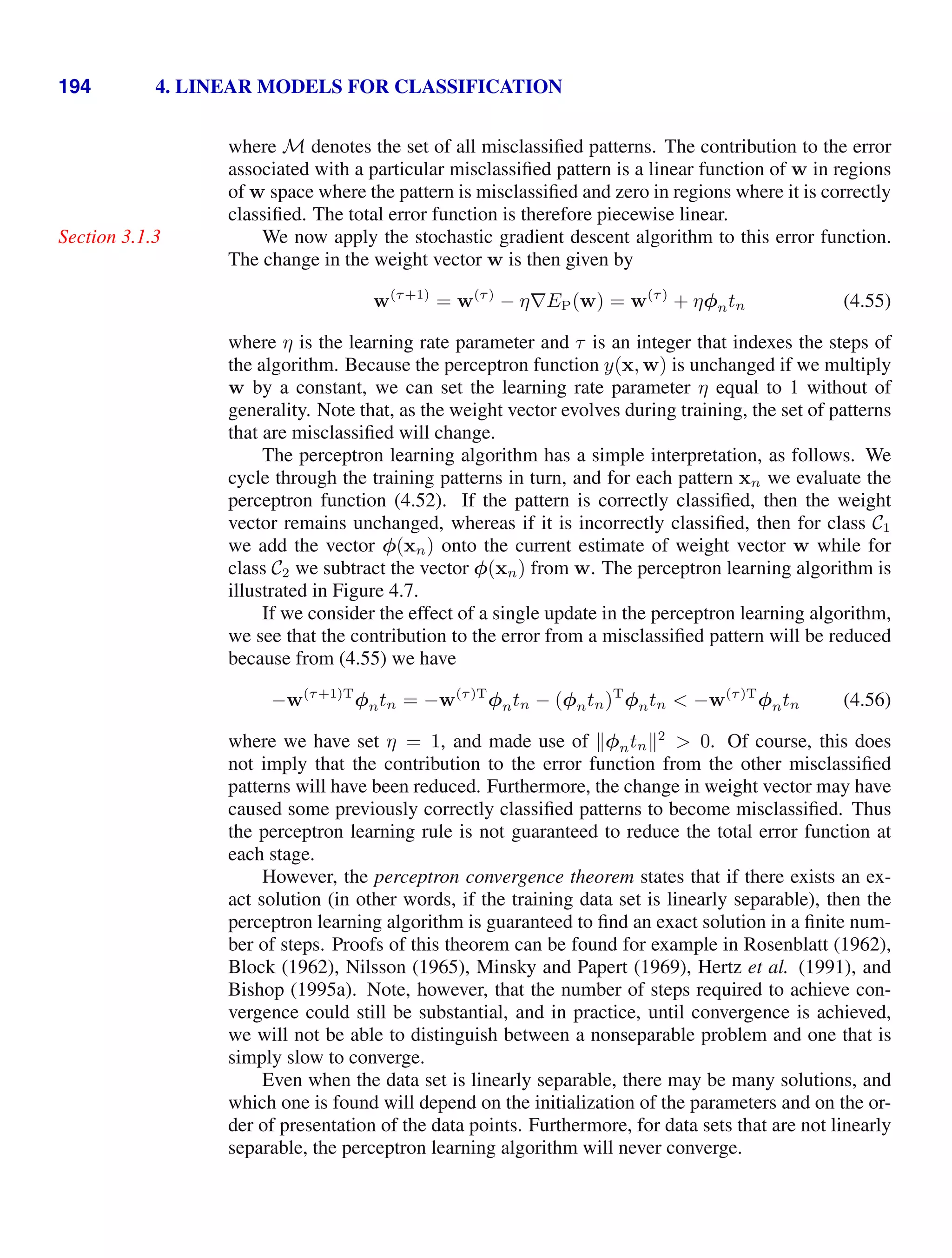
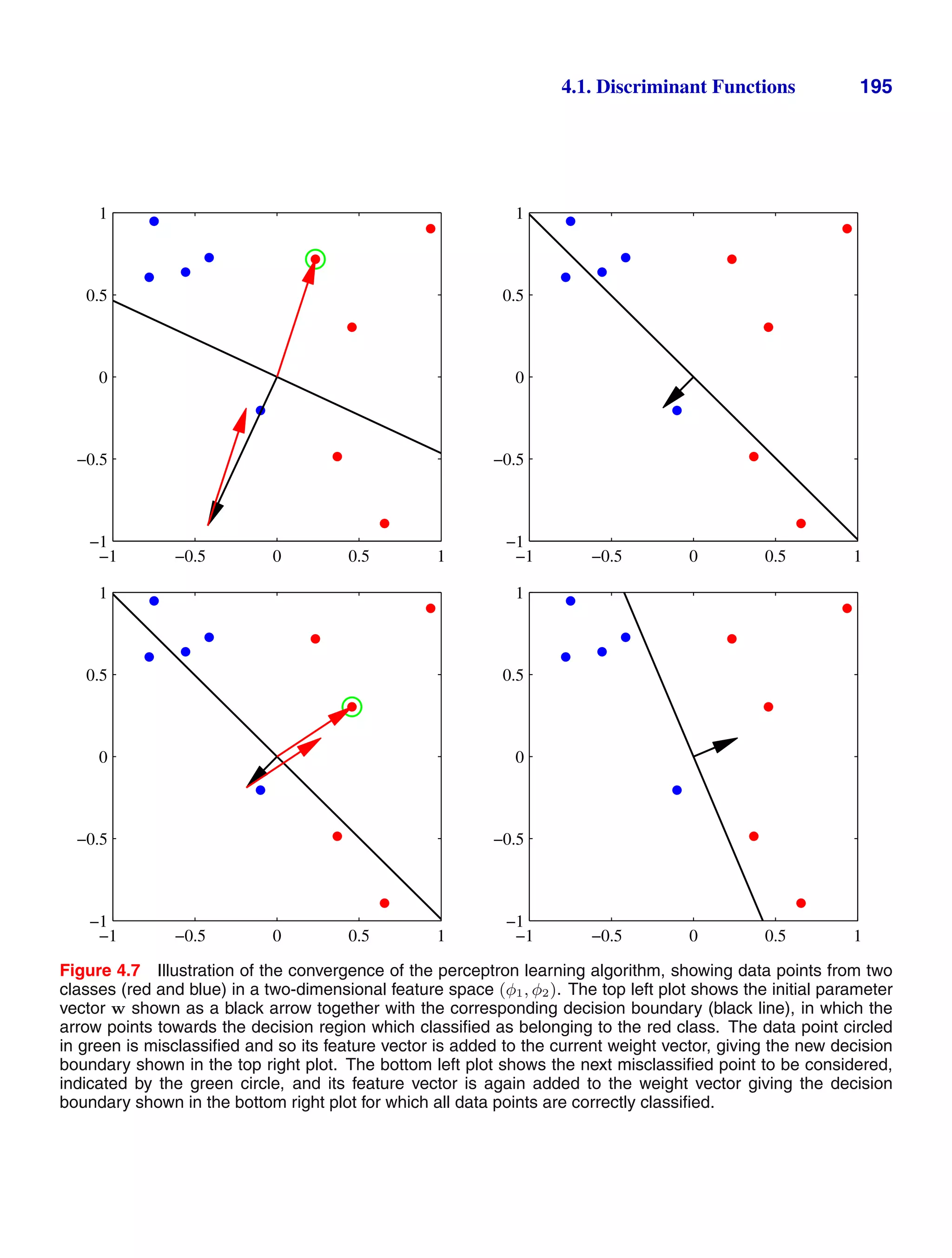
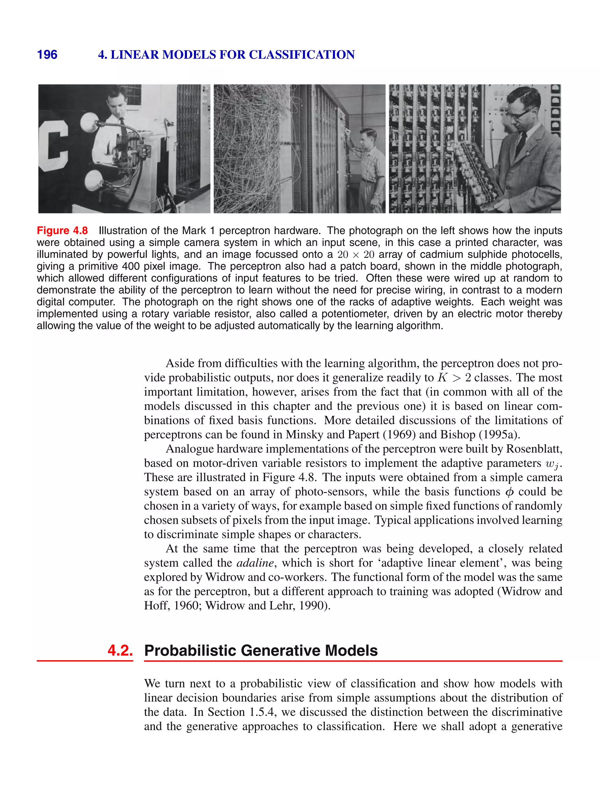
![4.2. Probabilistic Generative Models 197
Figure 4.9 Plot of the logistic sigmoid function
σ(a) defined by (4.59), shown in
red, together with the scaled pro-
bit function Φ(λa), for λ2
= π/8,
shown in dashed blue, where Φ(a)
is defined by (4.114). The scal-
ing factor π/8 is chosen so that the
derivatives of the two curves are
equal for a = 0.
−5 0 5
0
0.5
1
approach in which we model the class-conditional densities p(x|Ck), as well as the
class priors p(Ck), and then use these to compute posterior probabilities p(Ck|x)
through Bayes’ theorem.
Consider first of all the case of two classes. The posterior probability for class
C1 can be written as
p(C1|x) =
p(x|C1)p(C1)
p(x|C1)p(C1) + p(x|C2)p(C2)
=
1
1 + exp(−a)
= σ(a) (4.57)
where we have defined
a = ln
p(x|C1)p(C1)
p(x|C2)p(C2)
(4.58)
and σ(a) is the logistic sigmoid function defined by
σ(a) =
1
1 + exp(−a)
(4.59)
which is plotted in Figure 4.9. The term ‘sigmoid’ means S-shaped. This type of
function is sometimes also called a ‘squashing function’ because it maps the whole
real axis into a finite interval. The logistic sigmoid has been encountered already
in earlier chapters and plays an important role in many classification algorithms. It
satisfies the following symmetry property
σ(−a) = 1 − σ(a) (4.60)
as is easily verified. The inverse of the logistic sigmoid is given by
a = ln
σ
1 − σ
(4.61)
and is known as the logit function. It represents the log of the ratio of probabilities
ln [p(C1|x)/p(C2|x)] for the two classes, also known as the log odds.](https://image.slidesharecdn.com/bishop-patternrecognitionandmachinelearning-230316082240-9af1cdaa/75/Bishop-Pattern-Recognition-and-Machine-Learning-pdf-214-2048.jpg)
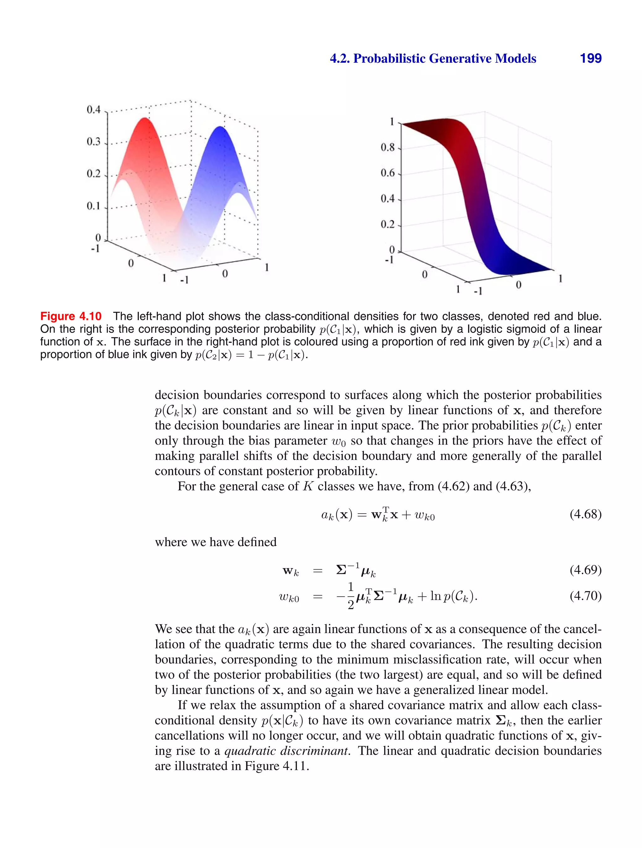
![200 4. LINEAR MODELS FOR CLASSIFICATION
−2 −1 0 1 2
−2.5
−2
−1.5
−1
−0.5
0
0.5
1
1.5
2
2.5
Figure 4.11 The left-hand plot shows the class-conditional densities for three classes each having a Gaussian
distribution, coloured red, green, and blue, in which the red and green classes have the same covariance matrix.
The right-hand plot shows the corresponding posterior probabilities, in which the RGB colour vector represents
the posterior probabilities for the respective three classes. The decision boundaries are also shown. Notice that
the boundary between the red and green classes, which have the same covariance matrix, is linear, whereas
those between the other pairs of classes are quadratic.
4.2.2 Maximum likelihood solution
Once we have specified a parametric functional form for the class-conditional
densities p(x|Ck), we can then determine the values of the parameters, together with
the prior class probabilities p(Ck), using maximum likelihood. This requires a data
set comprising observations of x along with their corresponding class labels.
Consider first the case of two classes, each having a Gaussian class-conditional
density with a shared covariance matrix, and suppose we have a data set {xn, tn}
where n = 1, . . . , N. Here tn = 1 denotes class C1 and tn = 0 denotes class C2. We
denote the prior class probability p(C1) = π, so that p(C2) = 1 − π. For a data point
xn from class C1, we have tn = 1 and hence
p(xn, C1) = p(C1)p(xn|C1) = πN(xn|µ1, Σ).
Similarly for class C2, we have tn = 0 and hence
p(xn, C2) = p(C2)p(xn|C2) = (1 − π)N(xn|µ2, Σ).
Thus the likelihood function is given by
p(t|π, µ1, µ2, Σ) =
N
n=1
[πN(xn|µ1, Σ)]
tn
[(1 − π)N(xn|µ2, Σ)]
1−tn
(4.71)
where t = (t1, . . . , tN )T
. As usual, it is convenient to maximize the log of the
likelihood function. Consider first the maximization with respect to π. The terms in](https://image.slidesharecdn.com/bishop-patternrecognitionandmachinelearning-230316082240-9af1cdaa/75/Bishop-Pattern-Recognition-and-Machine-Learning-pdf-217-2048.jpg)
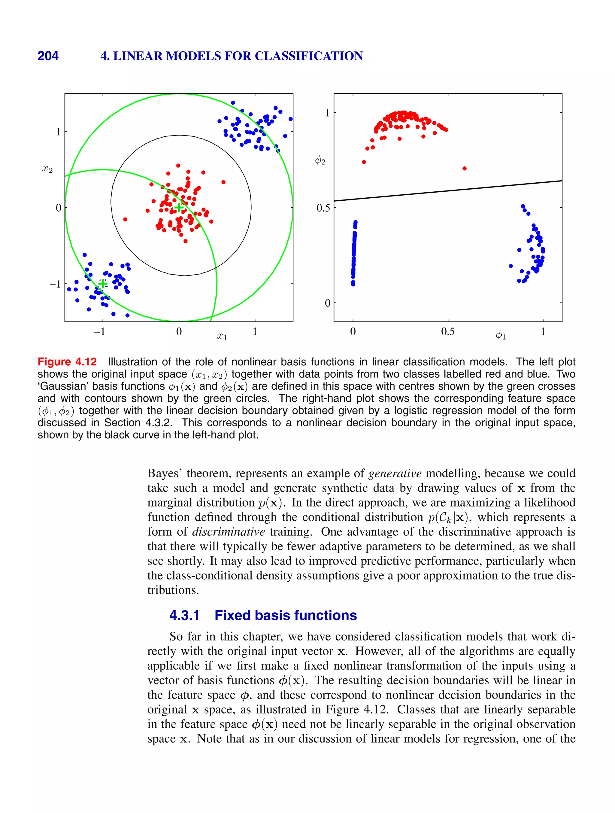
![208 4. LINEAR MODELS FOR CLASSIFICATION
where we have made use of (4.88). Also, we have introduced the N × N diagonal
matrix R with elements
Rnn = yn(1 − yn). (4.98)
We see that the Hessian is no longer constant but depends on w through the weight-
ing matrix R, corresponding to the fact that the error function is no longer quadratic.
Using the property 0 yn 1, which follows from the form of the logistic sigmoid
function, we see that uT
Hu 0 for an arbitrary vector u, and so the Hessian matrix
H is positive definite. It follows that the error function is a concave function of w
and hence has a unique minimum.
Exercise 4.15
The Newton-Raphson update formula for the logistic regression model then be-
comes
w(new)
= w(old)
− (ΦT
RΦ)−1
ΦT
(y − t)
= (ΦT
RΦ)−1
ΦT
RΦw(old)
− ΦT
(y − t)
= (ΦT
RΦ)−1
ΦT
Rz (4.99)
where z is an N-dimensional vector with elements
z = Φw(old)
− R−1
(y − t). (4.100)
We see that the update formula (4.99) takes the form of a set of normal equations for a
weighted least-squares problem. Because the weighing matrix R is not constant but
depends on the parameter vector w, we must apply the normal equations iteratively,
each time using the new weight vector w to compute a revised weighing matrix
R. For this reason, the algorithm is known as iterative reweighted least squares, or
IRLS (Rubin, 1983). As in the weighted least-squares problem, the elements of the
diagonal weighting matrix R can be interpreted as variances because the mean and
variance of t in the logistic regression model are given by
E[t] = σ(x) = y (4.101)
var[t] = E[t2
] − E[t]2
= σ(x) − σ(x)2
= y(1 − y) (4.102)
where we have used the property t2
= t for t ∈ {0, 1}. In fact, we can interpret IRLS
as the solution to a linearized problem in the space of the variable a = wT
φ. The
quantity zn, which corresponds to the nth
element of z, can then be given a simple
interpretation as an effective target value in this space obtained by making a local
linear approximation to the logistic sigmoid function around the current operating
point w(old)
an(w) an(w(old)
) +
dan
dyn
w(old)
(tn − yn)
= φT
nw(old)
−
(yn − tn)
yn(1 − yn)
= zn. (4.103)](https://image.slidesharecdn.com/bishop-patternrecognitionandmachinelearning-230316082240-9af1cdaa/75/Bishop-Pattern-Recognition-and-Machine-Learning-pdf-225-2048.jpg)
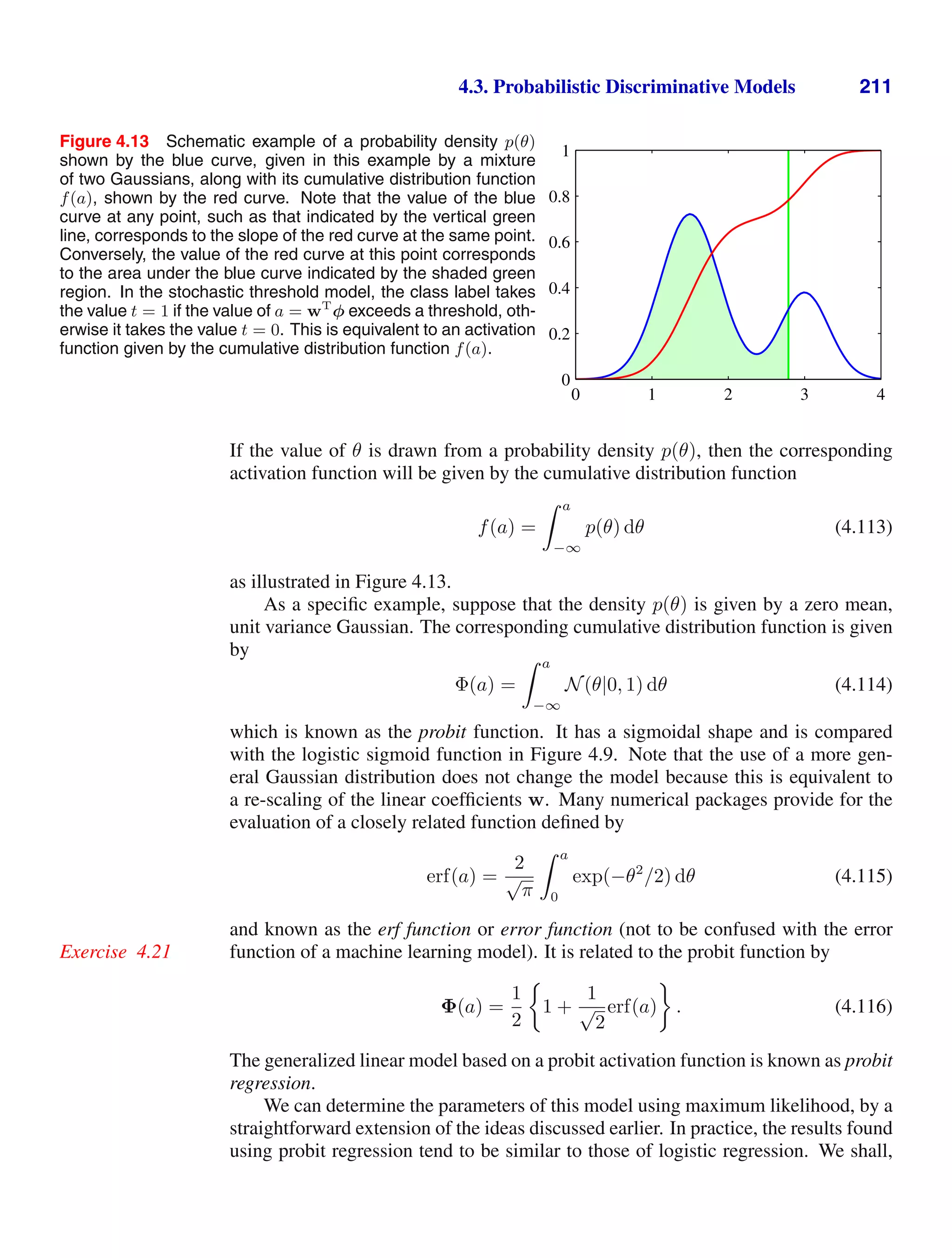
![212 4. LINEAR MODELS FOR CLASSIFICATION
however, find another use for the probit model when we discuss Bayesian treatments
of logistic regression in Section 4.5.
One issue that can occur in practical applications is that of outliers, which can
arise for instance through errors in measuring the input vector x or through misla-
belling of the target value t. Because such points can lie a long way to the wrong side
of the ideal decision boundary, they can seriously distort the classifier. Note that the
logistic and probit regression models behave differently in this respect because the
tails of the logistic sigmoid decay asymptotically like exp(−x) for x → ∞, whereas
for the probit activation function they decay like exp(−x2
), and so the probit model
can be significantly more sensitive to outliers.
However, both the logistic and the probit models assume the data is correctly
labelled. The effect of mislabelling is easily incorporated into a probabilistic model
by introducing a probability that the target value t has been flipped to the wrong
value (Opper and Winther, 2000a), leading to a target value distribution for data point
x of the form
p(t|x) = (1 − )σ(x) + (1 − σ(x))
= + (1 − 2)σ(x) (4.117)
where σ(x) is the activation function with input vector x. Here may be set in
advance, or it may be treated as a hyperparameter whose value is inferred from the
data.
4.3.6 Canonical link functions
For the linear regression model with a Gaussian noise distribution, the error
function, corresponding to the negative log likelihood, is given by (3.12). If we take
the derivative with respect to the parameter vector w of the contribution to the error
function from a data point n, this takes the form of the ‘error’ yn − tn times the
feature vector φn, where yn = wT
φn. Similarly, for the combination of the logistic
sigmoid activation function and the cross-entropy error function (4.90), and for the
softmax activation function with the multiclass cross-entropy error function (4.108),
we again obtain this same simple form. We now show that this is a general result
of assuming a conditional distribution for the target variable from the exponential
family, along with a corresponding choice for the activation function known as the
canonical link function.
We again make use of the restricted form (4.84) of exponential family distribu-
tions. Note that here we are applying the assumption of exponential family distribu-
tion to the target variable t, in contrast to Section 4.2.4 where we applied it to the
input vector x. We therefore consider conditional distributions of the target variable
of the form
p(t|η, s) =
1
s
h
t
s
g(η) exp
ηt
s
. (4.118)
Using the same line of argument as led to the derivation of the result (2.226), we see
that the conditional mean of t, which we denote by y, is given by
y ≡ E[t|η] = −s
d
dη
ln g(η). (4.119)](https://image.slidesharecdn.com/bishop-patternrecognitionandmachinelearning-230316082240-9af1cdaa/75/Bishop-Pattern-Recognition-and-Machine-Learning-pdf-229-2048.jpg)
![4.4. The Laplace Approximation 213
Thus y and η must related, and we denote this relation through η = ψ(y).
Following Nelder and Wedderburn (1972), we define a generalized linear model
to be one for which y is a nonlinear function of a linear combination of the input (or
feature) variables so that
y = f(wT
φ) (4.120)
where f(·) is known as the activation function in the machine learning literature, and
f−1
(·) is known as the link function in statistics.
Now consider the log likelihood function for this model, which, as a function of
η, is given by
ln p(t|η, s) =
N
n=1
ln p(tn|η, s) =
N
n=1
ln g(ηn) +
ηntn
s
+ const (4.121)
where we are assuming that all observations share a common scale parameter (which
corresponds to the noise variance for a Gaussian distribution for instance) and so s
is independent of n. The derivative of the log likelihood with respect to the model
parameters w is then given by
∇w ln p(t|η, s) =
N
n=1
d
dηn
ln g(ηn) +
tn
s
dηn
dyn
dyn
dan
∇an
=
N
n=1
1
s
{tn − yn} ψ
(yn)f
(an)φn (4.122)
where an = wT
φn, and we have used yn = f(an) together with the result (4.119)
for E[t|η]. We now see that there is a considerable simplification if we choose a
particular form for the link function f−1
(y) given by
f−1
(y) = ψ(y) (4.123)
which gives f(ψ(y)) = y and hence f
(ψ)ψ
(y) = 1. Also, because a = f−1
(y),
we have a = ψ and hence f
(a)ψ
(y) = 1. In this case, the gradient of the error
function reduces to
∇ ln E(w) =
1
s
N
n=1
{yn − tn}φn. (4.124)
For the Gaussian s = β−1
, whereas for the logistic model s = 1.
4.4. The Laplace Approximation
In Section 4.5 we shall discuss the Bayesian treatment of logistic regression. As
we shall see, this is more complex than the Bayesian treatment of linear regression
models, discussed in Sections 3.3 and 3.5. In particular, we cannot integrate exactly](https://image.slidesharecdn.com/bishop-patternrecognitionandmachinelearning-230316082240-9af1cdaa/75/Bishop-Pattern-Recognition-and-Machine-Learning-pdf-230-2048.jpg)
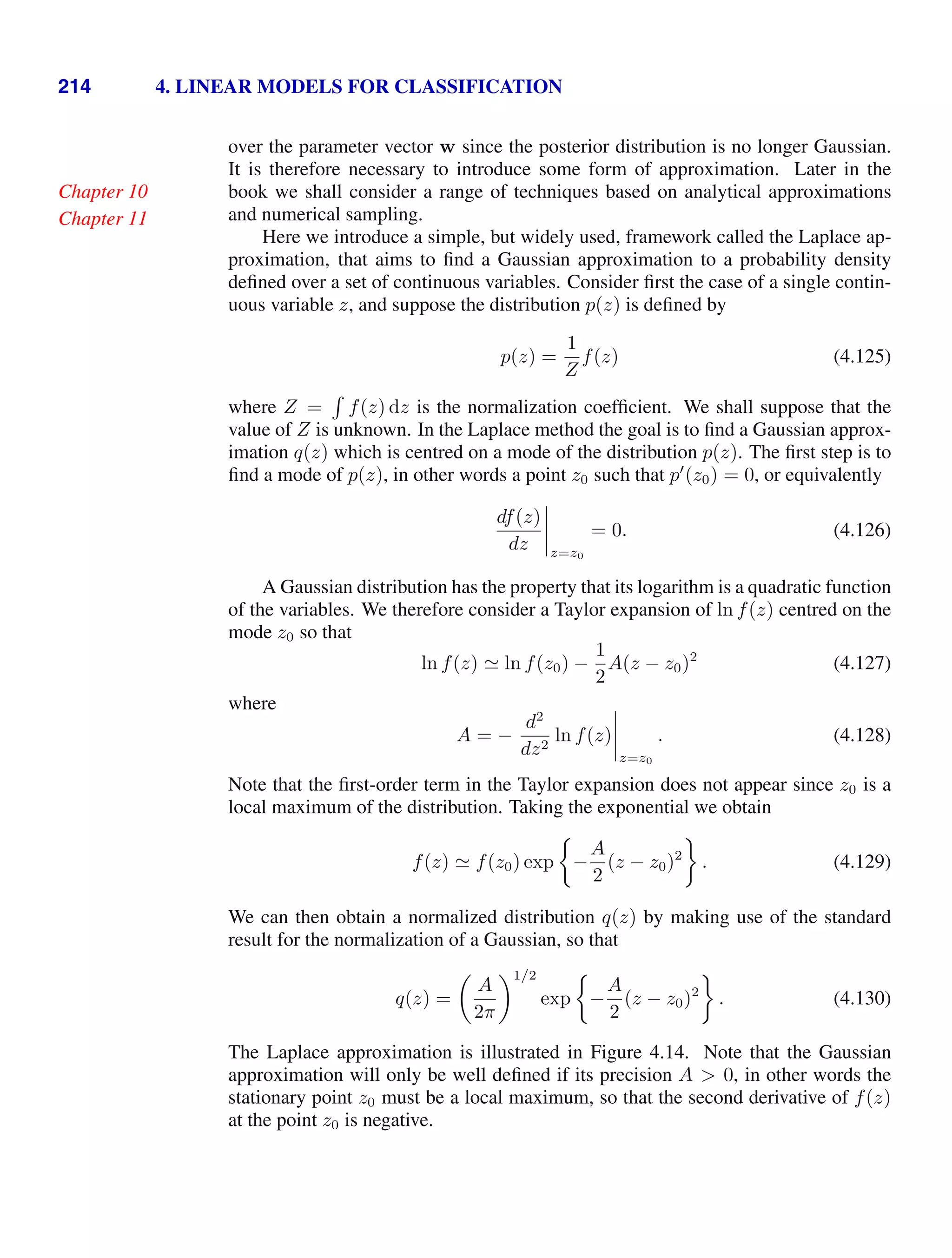
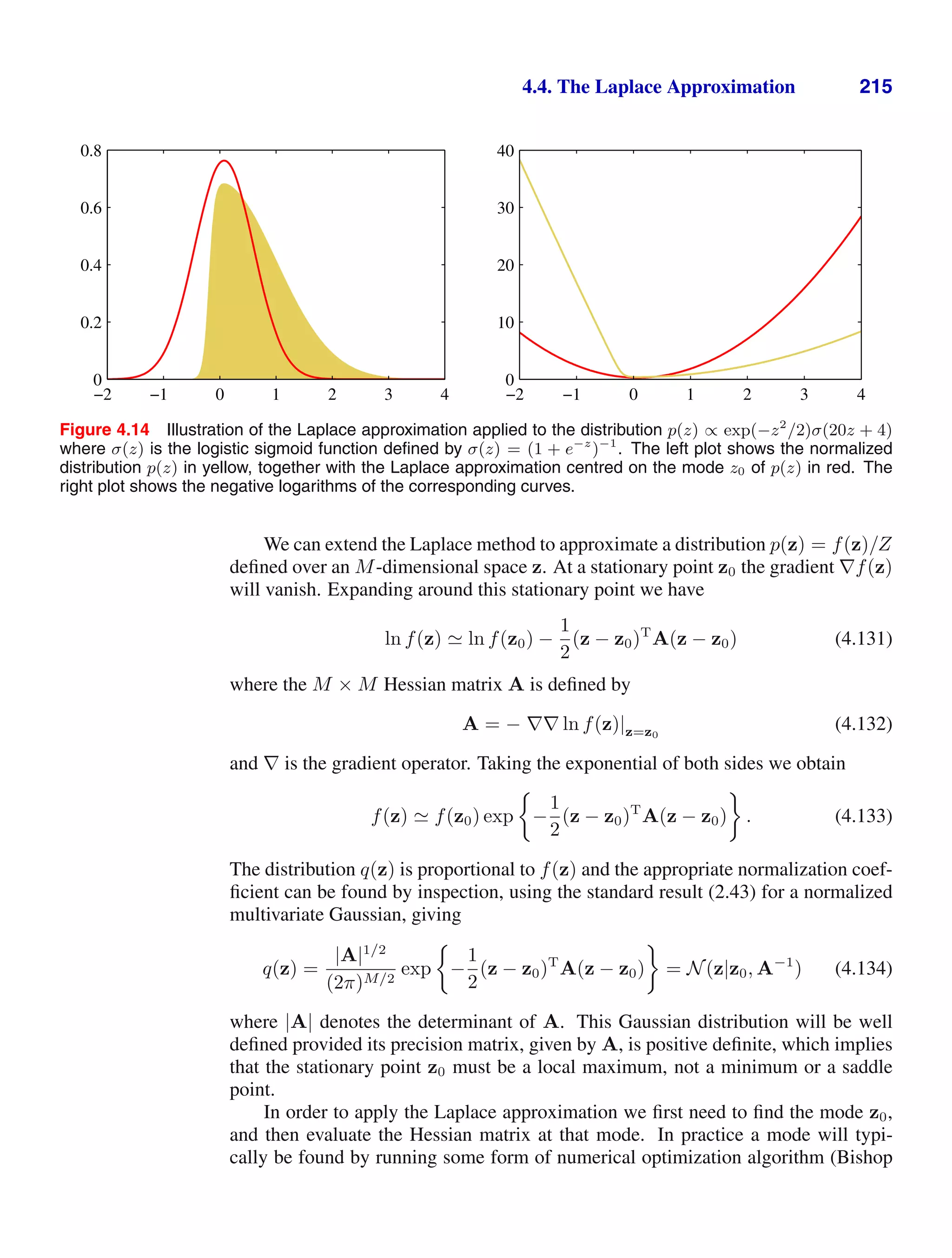
![4.5. Bayesian Logistic Regression 219
where
p(a) =
δ(a − wT
φ)q(w) dw. (4.148)
We can evaluate p(a) by noting that the delta function imposes a linear constraint
on w and so forms a marginal distribution from the joint distribution q(w) by inte-
grating out all directions orthogonal to φ. Because q(w) is Gaussian, we know from
Section 2.3.2 that the marginal distribution will also be Gaussian. We can evaluate
the mean and covariance of this distribution by taking moments, and interchanging
the order of integration over a and w, so that
µa = E[a] =
p(a)a da =
q(w)wT
φ dw = wT
MAPφ (4.149)
where we have used the result (4.144) for the variational posterior distribution q(w).
Similarly
σ2
a = var[a] =
p(a)
a2
− E[a]2
da
=
q(w)
(wT
φ)2
− (mT
N φ)2
dw = φT
SN φ. (4.150)
Note that the distribution of a takes the same form as the predictive distribution
(3.58) for the linear regression model, with the noise variance set to zero. Thus our
variational approximation to the predictive distribution becomes
p(C1|t) =
σ(a)p(a) da =
σ(a)N(a|µa, σ2
a) da. (4.151)
This result can also be derived directly by making use of the results for the marginal
of a Gaussian distribution given in Section 2.3.2.
Exercise 4.24
The integral over a represents the convolution of a Gaussian with a logistic sig-
moid, and cannot be evaluated analytically. We can, however, obtain a good approx-
imation (Spiegelhalter and Lauritzen, 1990; MacKay, 1992b; Barber and Bishop,
1998a) by making use of the close similarity between the logistic sigmoid function
σ(a) defined by (4.59) and the probit function Φ(a) defined by (4.114). In order to
obtain the best approximation to the logistic function we need to re-scale the hori-
zontal axis, so that we approximate σ(a) by Φ(λa). We can find a suitable value of
λ by requiring that the two functions have the same slope at the origin, which gives
λ2
= π/8. The similarity of the logistic sigmoid and the probit function, for this
Exercise 4.25
choice of λ, is illustrated in Figure 4.9.
The advantage of using a probit function is that its convolution with a Gaussian
can be expressed analytically in terms of another probit function. Specifically we
can show that
Exercise 4.26
Φ(λa)N(a|µ, σ2
) da = Φ
µ
(λ−2 + σ2)1/2
. (4.152)](https://image.slidesharecdn.com/bishop-patternrecognitionandmachinelearning-230316082240-9af1cdaa/75/Bishop-Pattern-Recognition-and-Machine-Learning-pdf-236-2048.jpg)

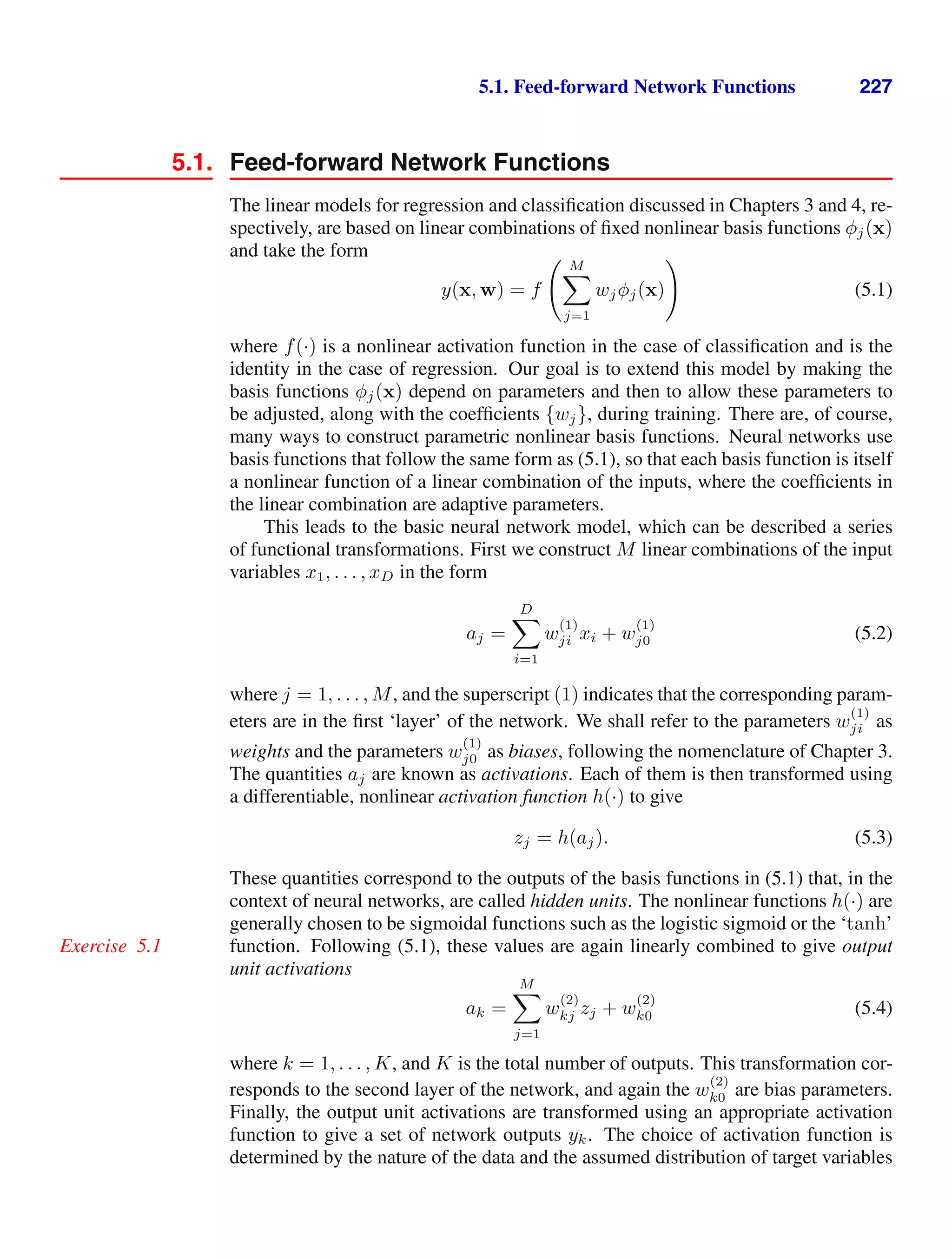
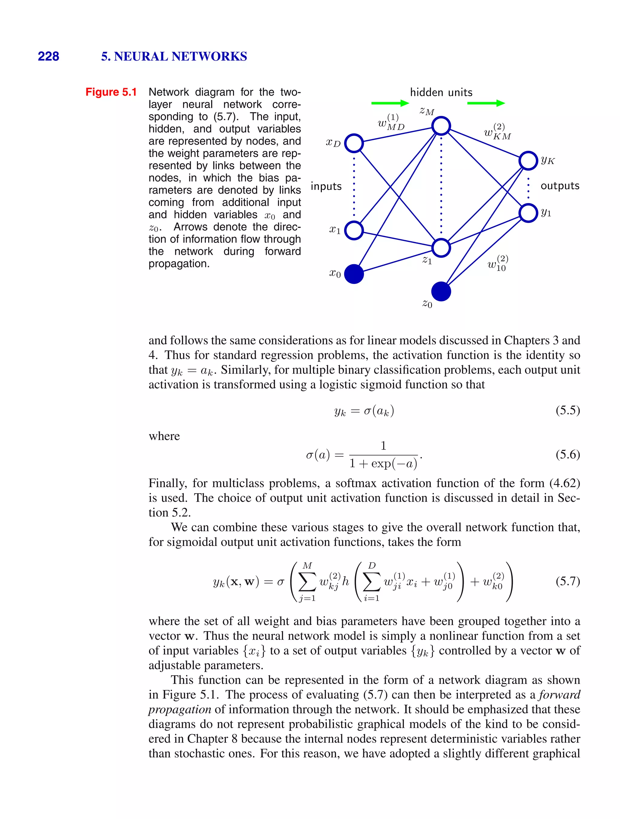
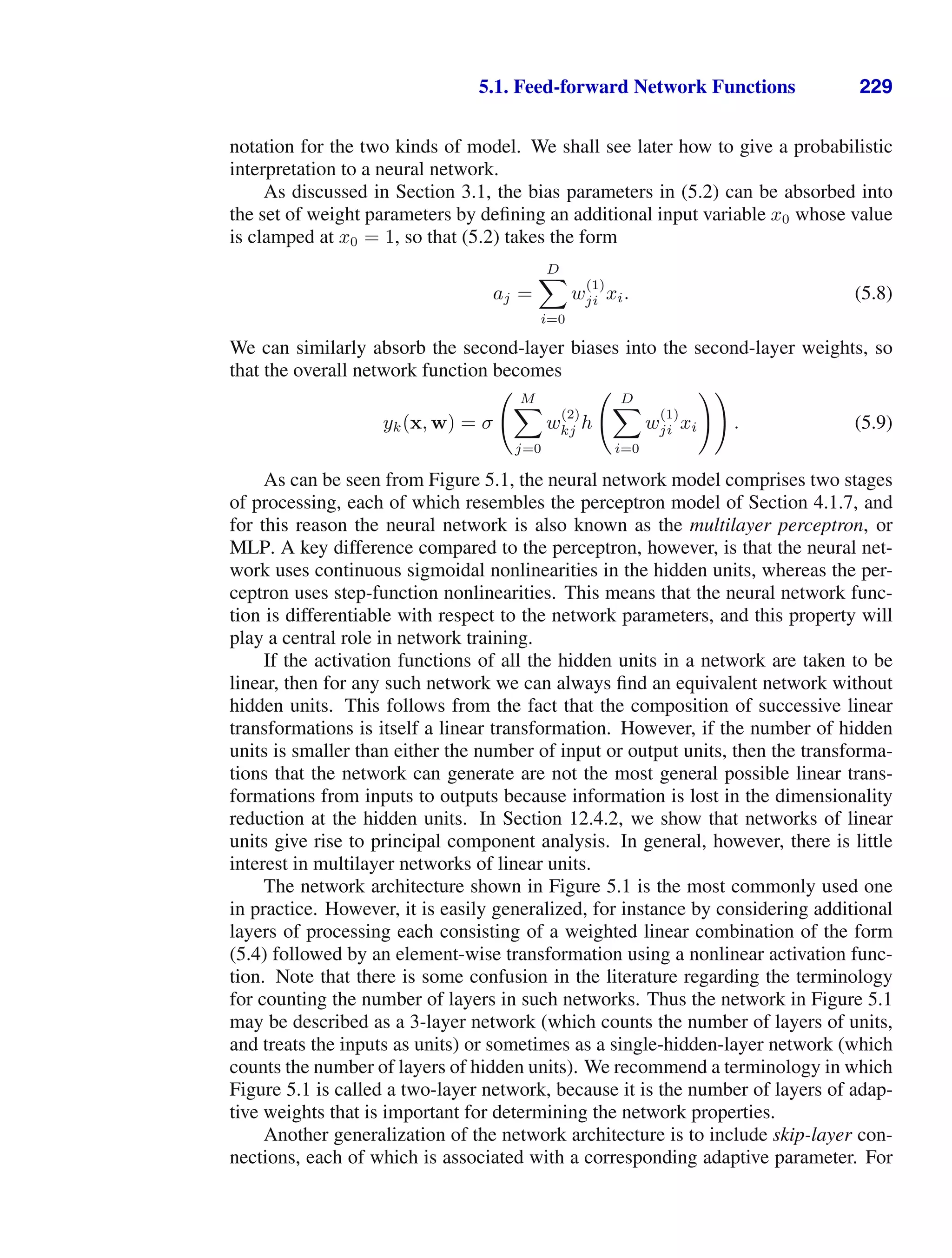
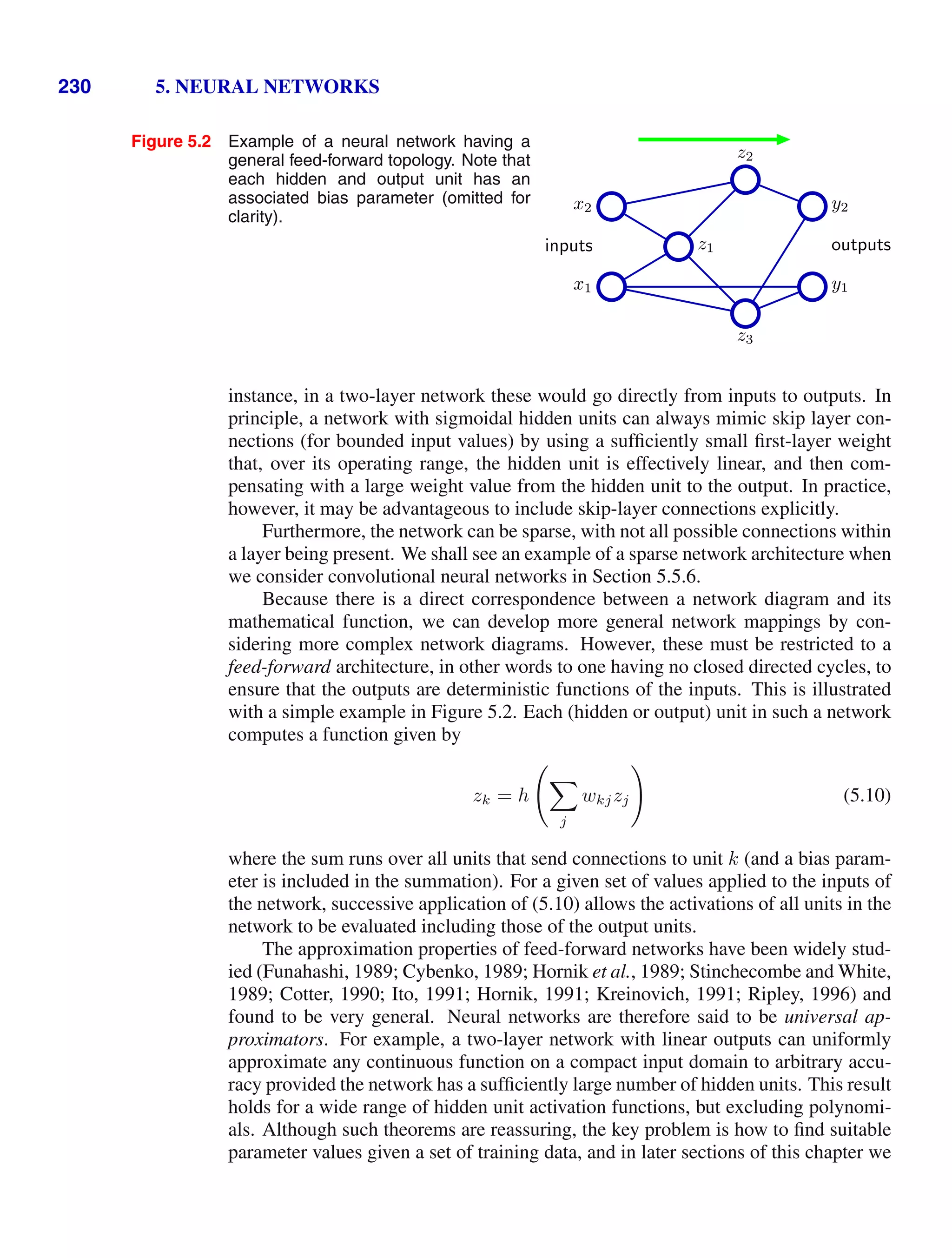
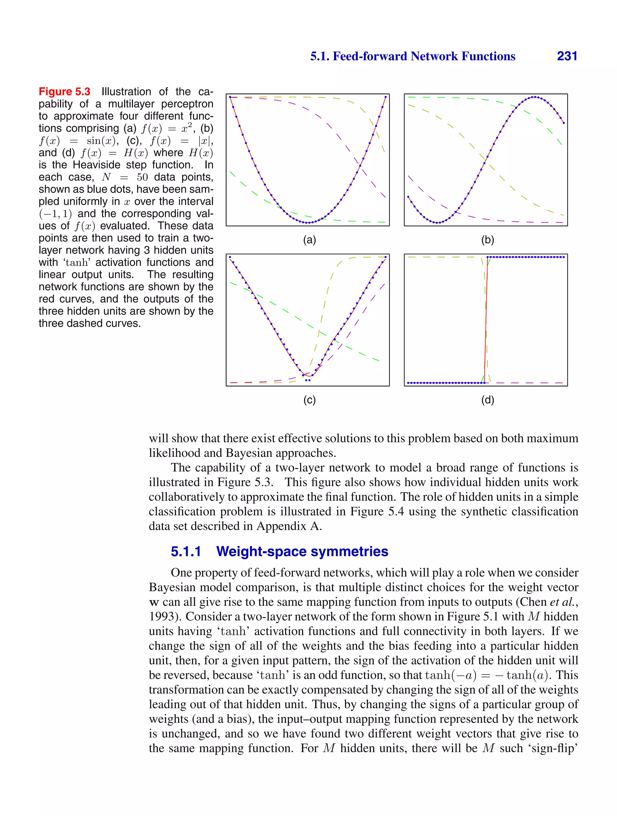
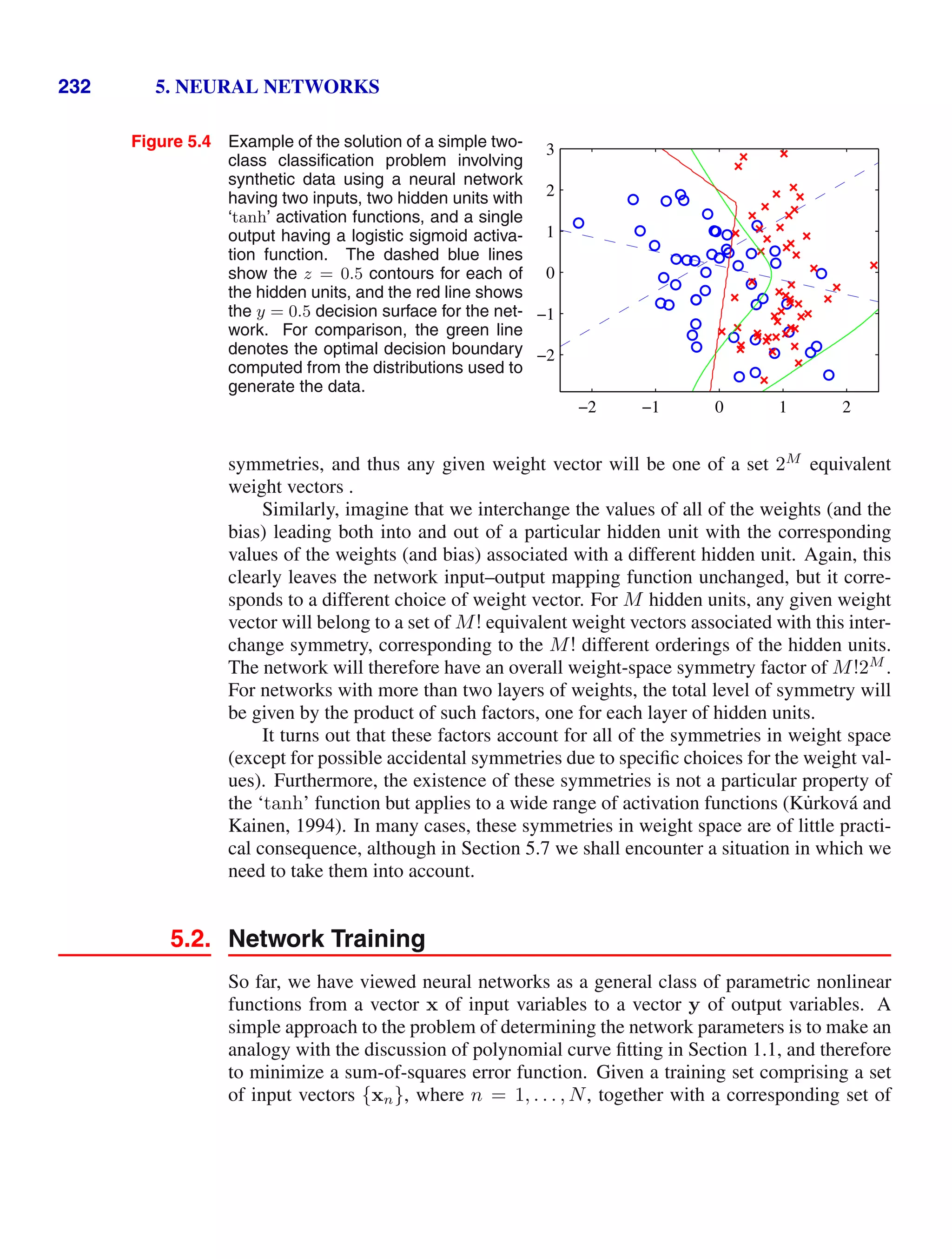
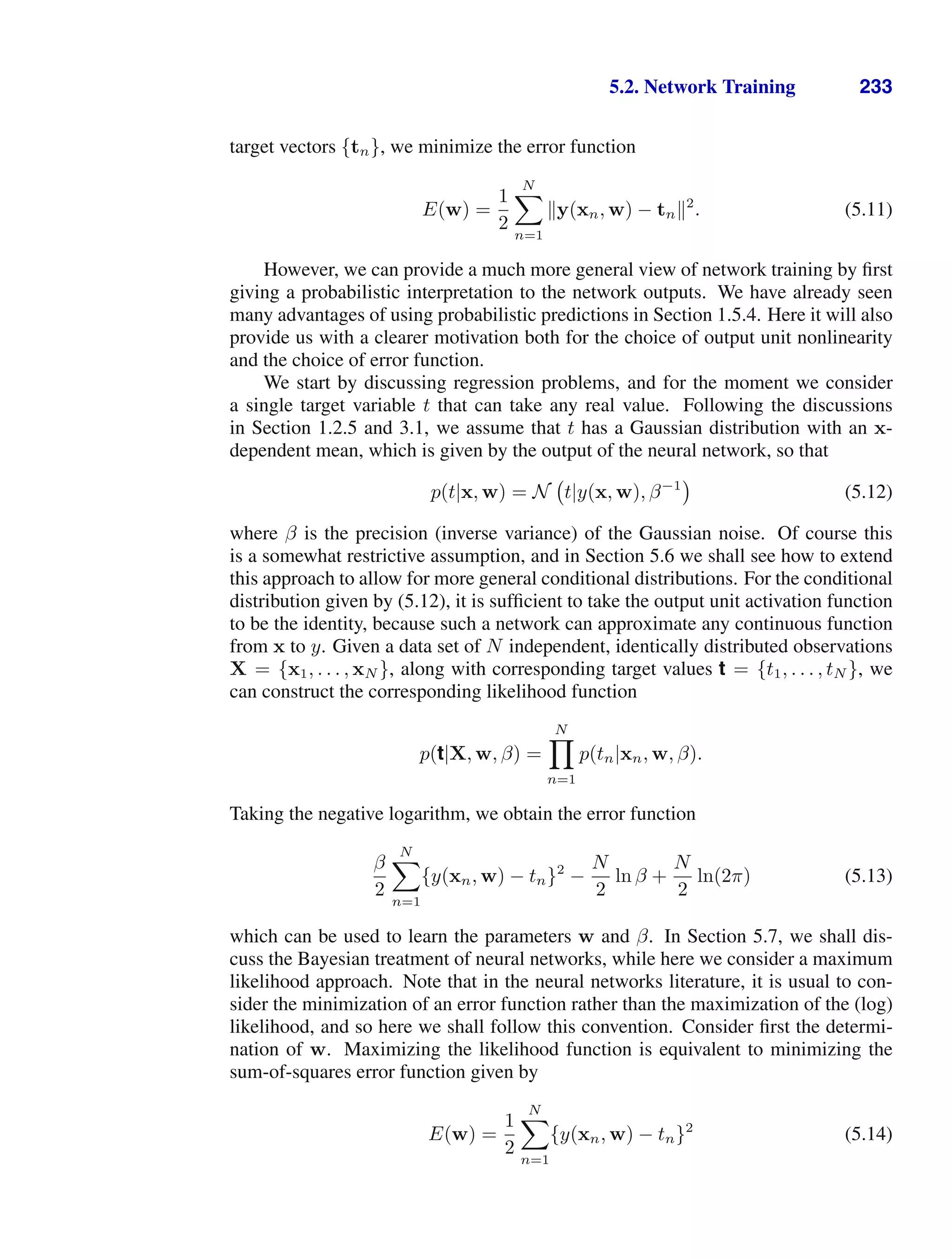
![5.2. Network Training 235
If we consider a training set of independent observations, then the error function,
which is given by the negative log likelihood, is then a cross-entropy error function
of the form
E(w) = −
N
n=1
{tn ln yn + (1 − tn) ln(1 − yn)} (5.21)
where yn denotes y(xn, w). Note that there is no analogue of the noise precision β
because the target values are assumed to be correctly labelled. However, the model
is easily extended to allow for labelling errors. Simard et al. (2003) found that using
Exercise 5.4
the cross-entropy error function instead of the sum-of-squares for a classification
problem leads to faster training as well as improved generalization.
If we have K separate binary classifications to perform, then we can use a net-
work having K outputs each of which has a logistic sigmoid activation function.
Associated with each output is a binary class label tk ∈ {0, 1}, where k = 1, . . . , K.
If we assume that the class labels are independent, given the input vector, then the
conditional distribution of the targets is
p(t|x, w) =
K
k=1
yk(x, w)tk
[1 − yk(x, w)]
1−tk
. (5.22)
Taking the negative logarithm of the corresponding likelihood function then gives
the following error function
Exercise 5.5
E(w) = −
N
n=1
K
k=1
{tnk ln ynk + (1 − tnk) ln(1 − ynk)} (5.23)
where ynk denotes yk(xn, w). Again, the derivative of the error function with re-
spect to the activation for a particular output unit takes the form (5.18) just as in the
Exercise 5.6
regression case.
It is interesting to contrast the neural network solution to this problem with the
corresponding approach based on a linear classification model of the kind discussed
in Chapter 4. Suppose that we are using a standard two-layer network of the kind
shown in Figure 5.1. We see that the weight parameters in the first layer of the
network are shared between the various outputs, whereas in the linear model each
classification problem is solved independently. The first layer of the network can
be viewed as performing a nonlinear feature extraction, and the sharing of features
between the different outputs can save on computation and can also lead to improved
generalization.
Finally, we consider the standard multiclass classification problem in which each
input is assigned to one of K mutually exclusive classes. The binary target variables
tk ∈ {0, 1} have a 1-of-K coding scheme indicating the class, and the network
outputs are interpreted as yk(x, w) = p(tk = 1|x), leading to the following error
function
E(w) = −
N
n=1
K
k=1
tkn ln yk(xn, w). (5.24)](https://image.slidesharecdn.com/bishop-patternrecognitionandmachinelearning-230316082240-9af1cdaa/75/Bishop-Pattern-Recognition-and-Machine-Learning-pdf-252-2048.jpg)
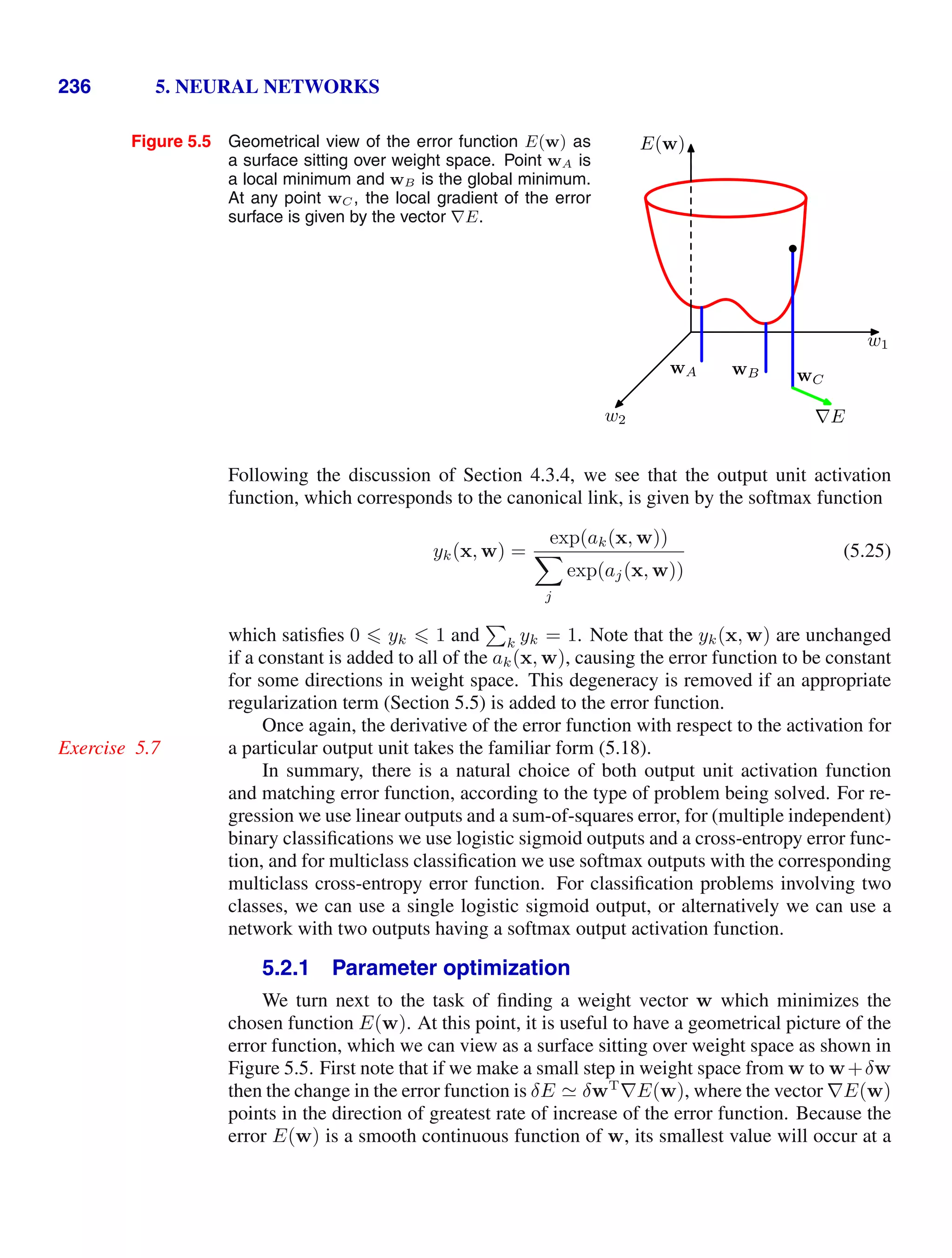
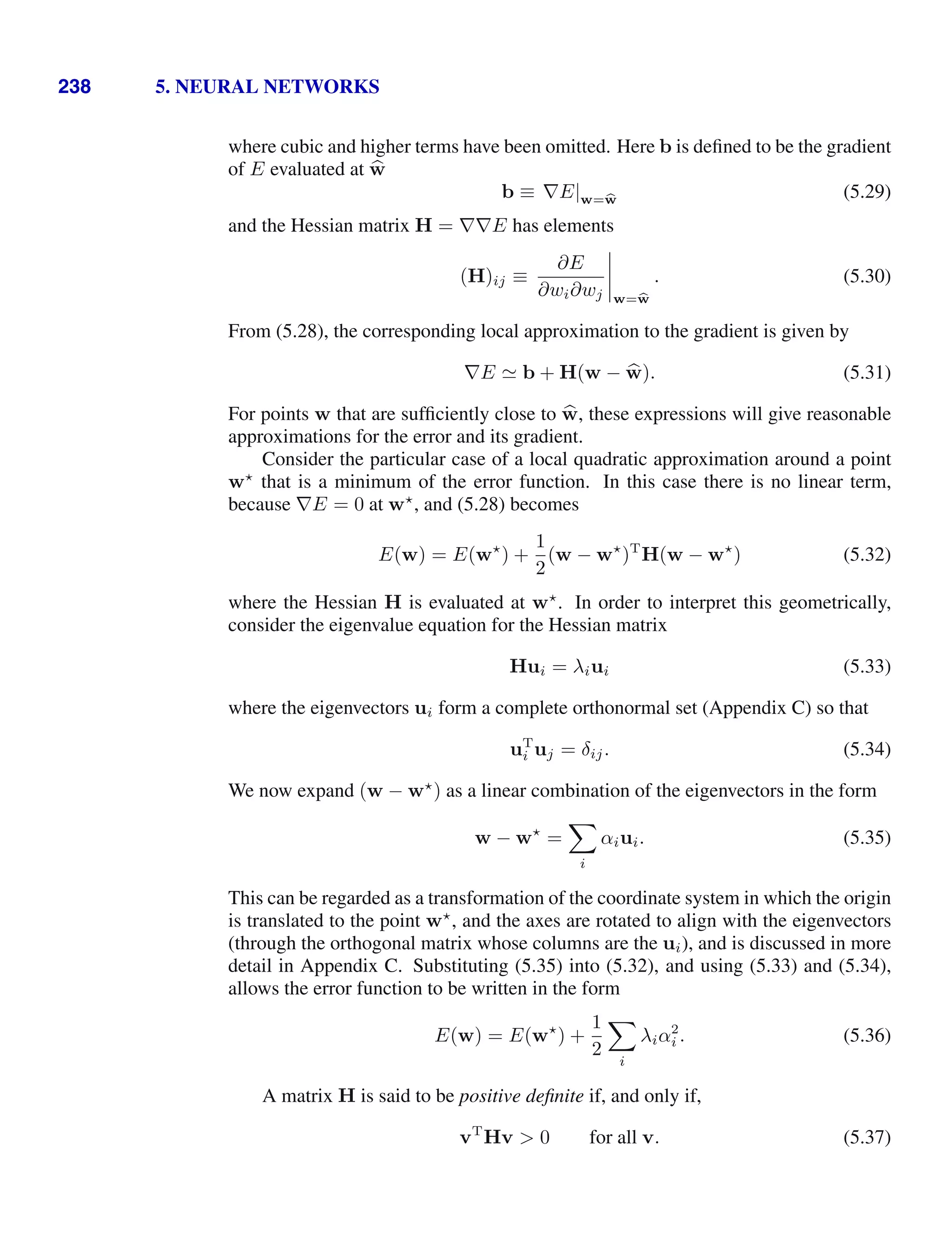
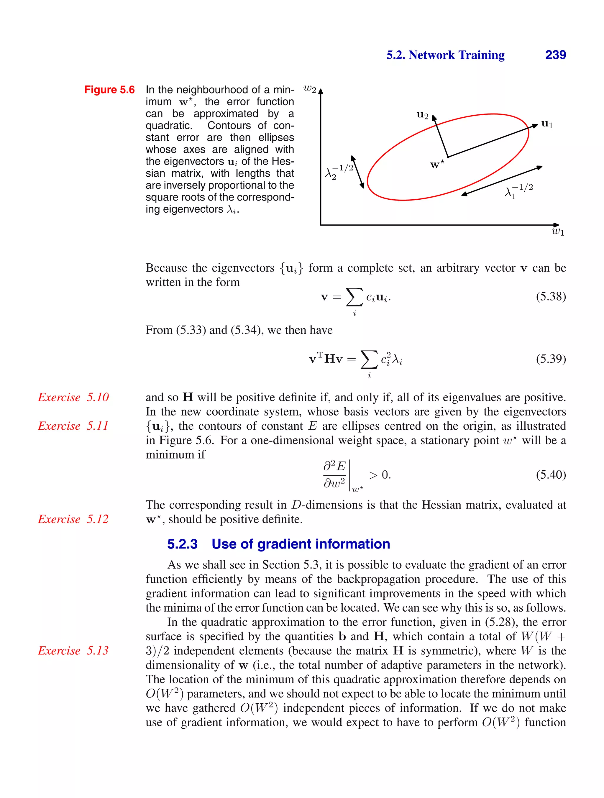
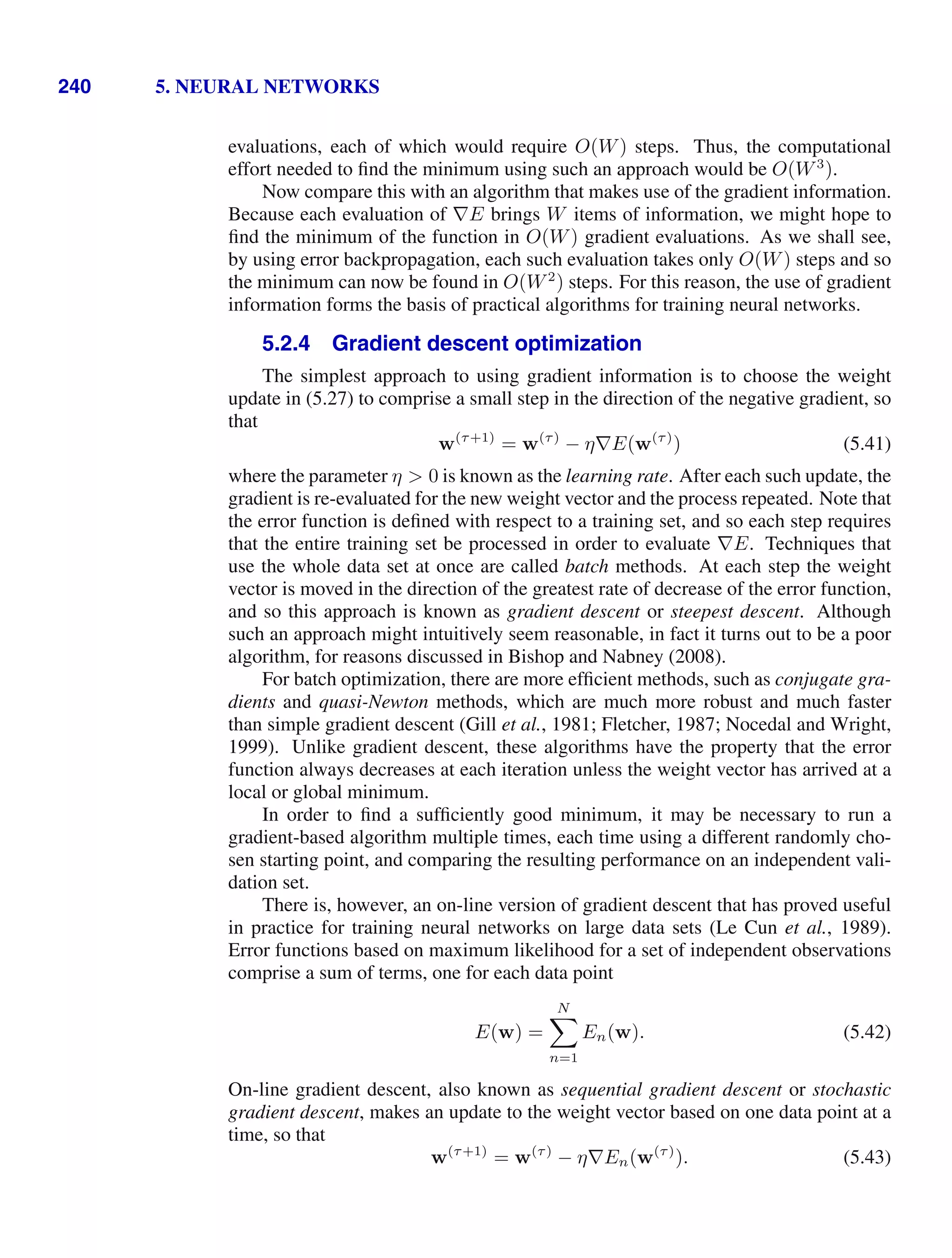
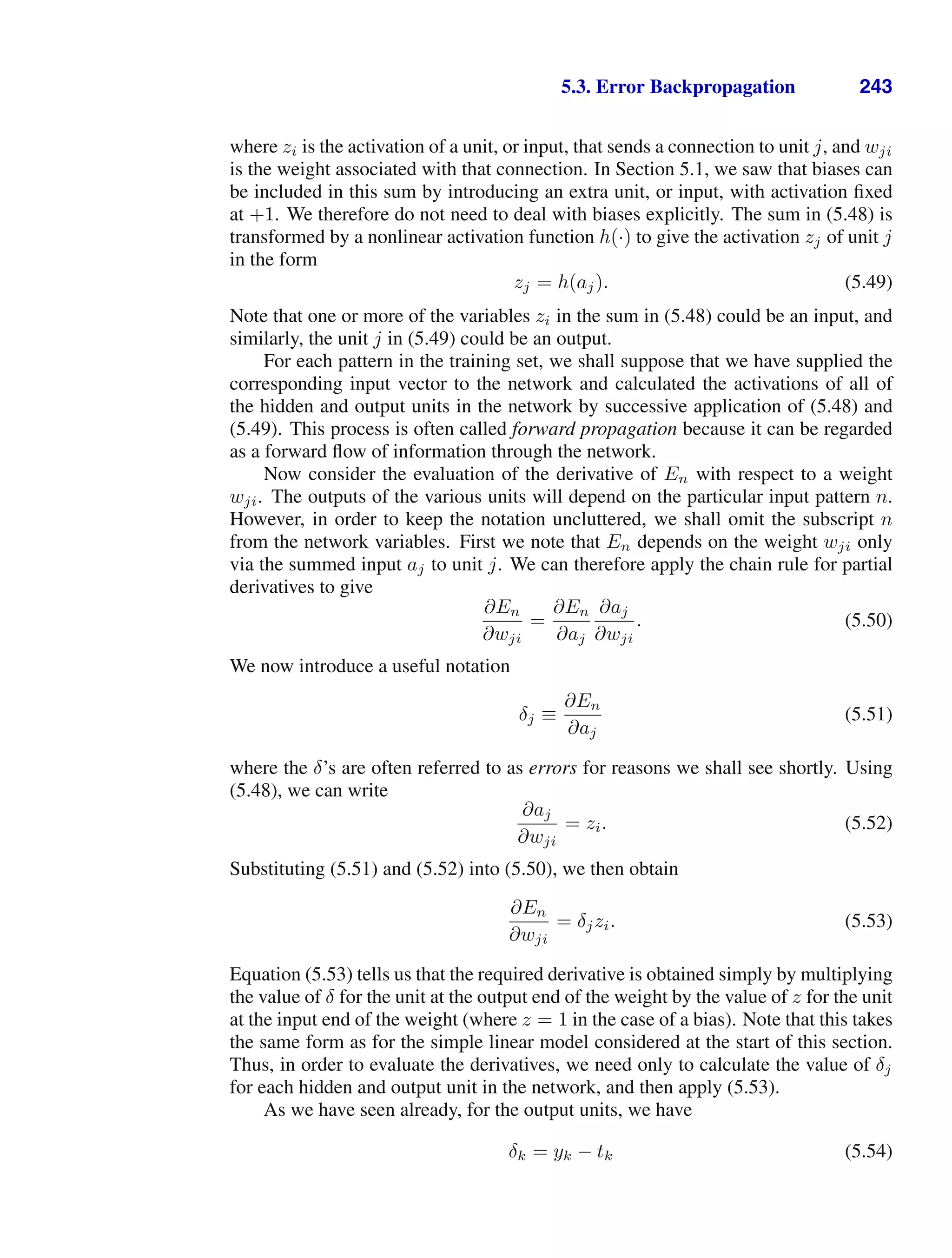
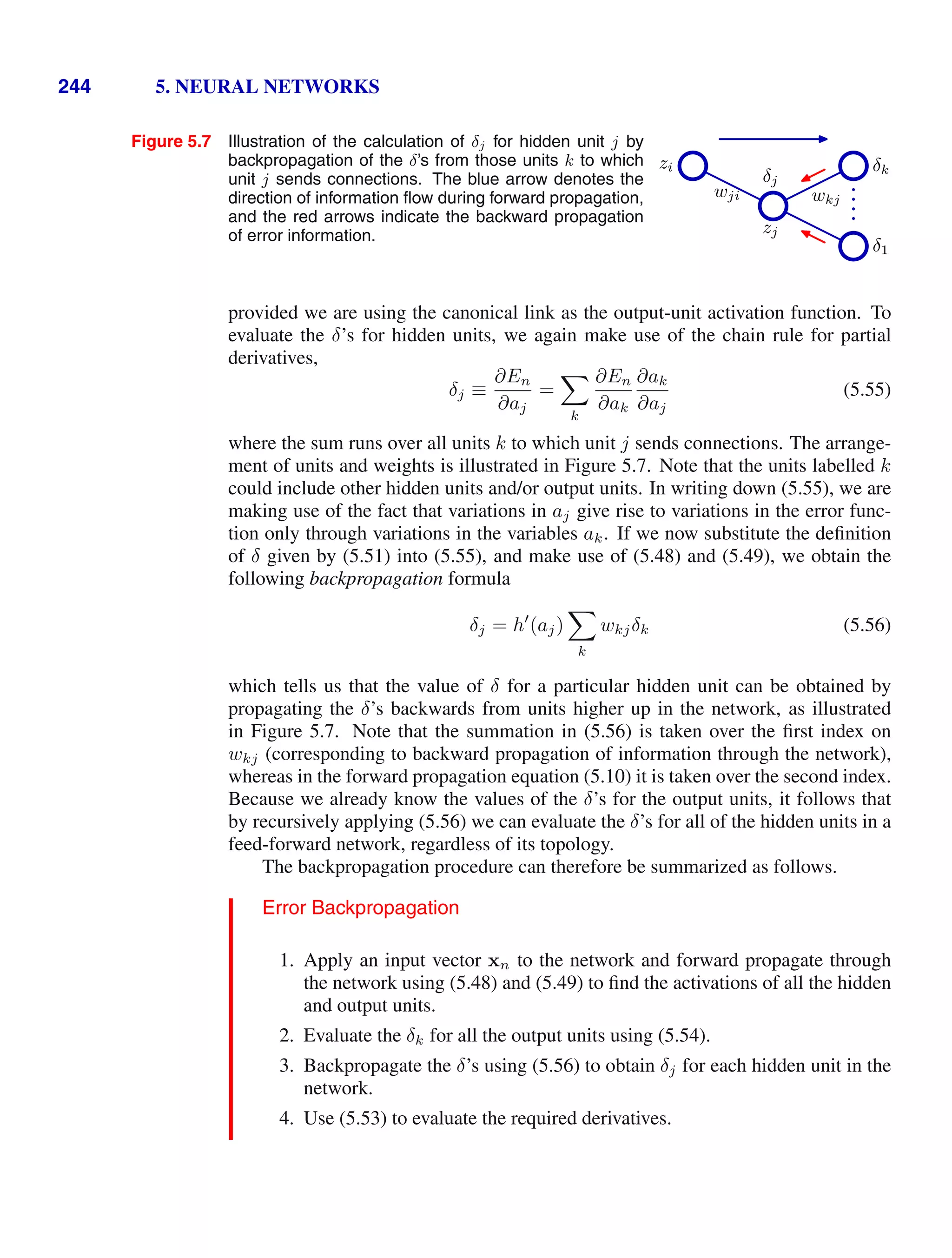
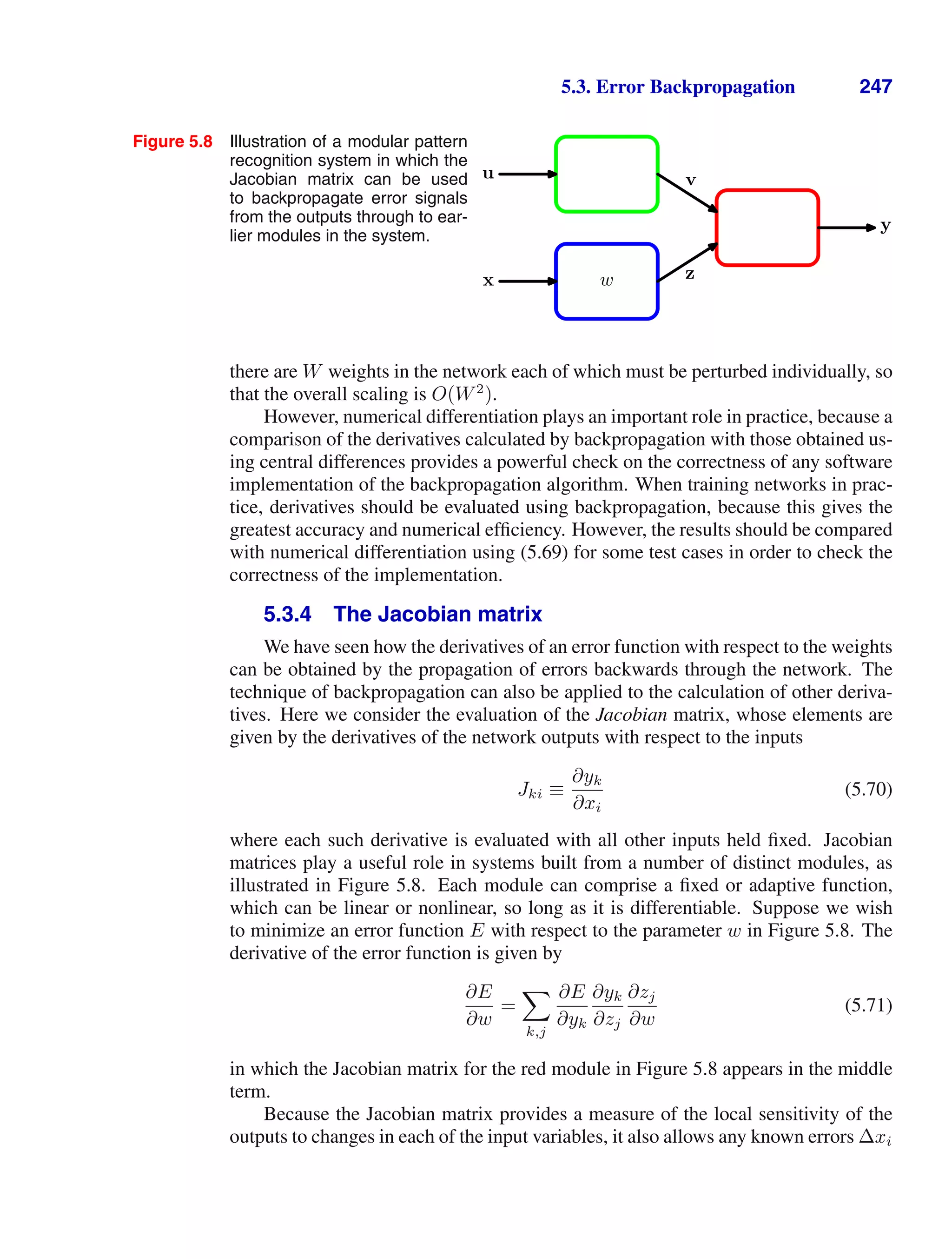
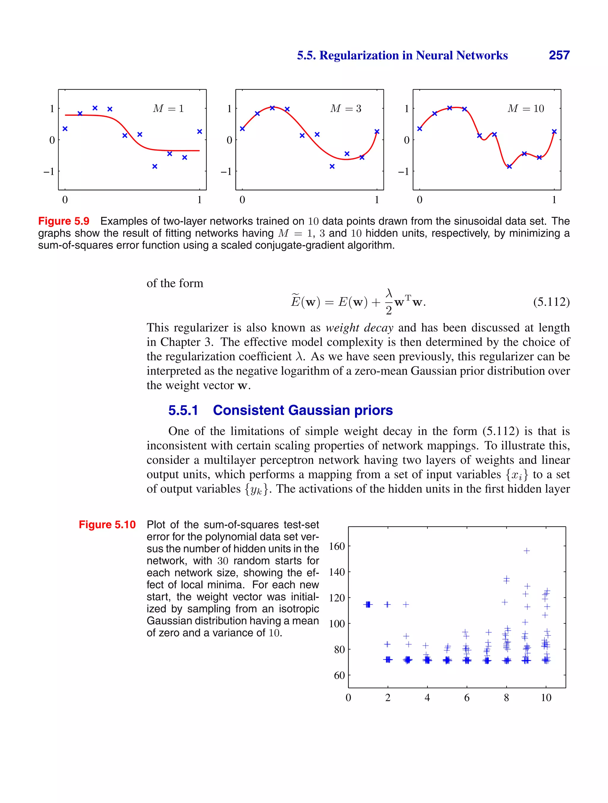
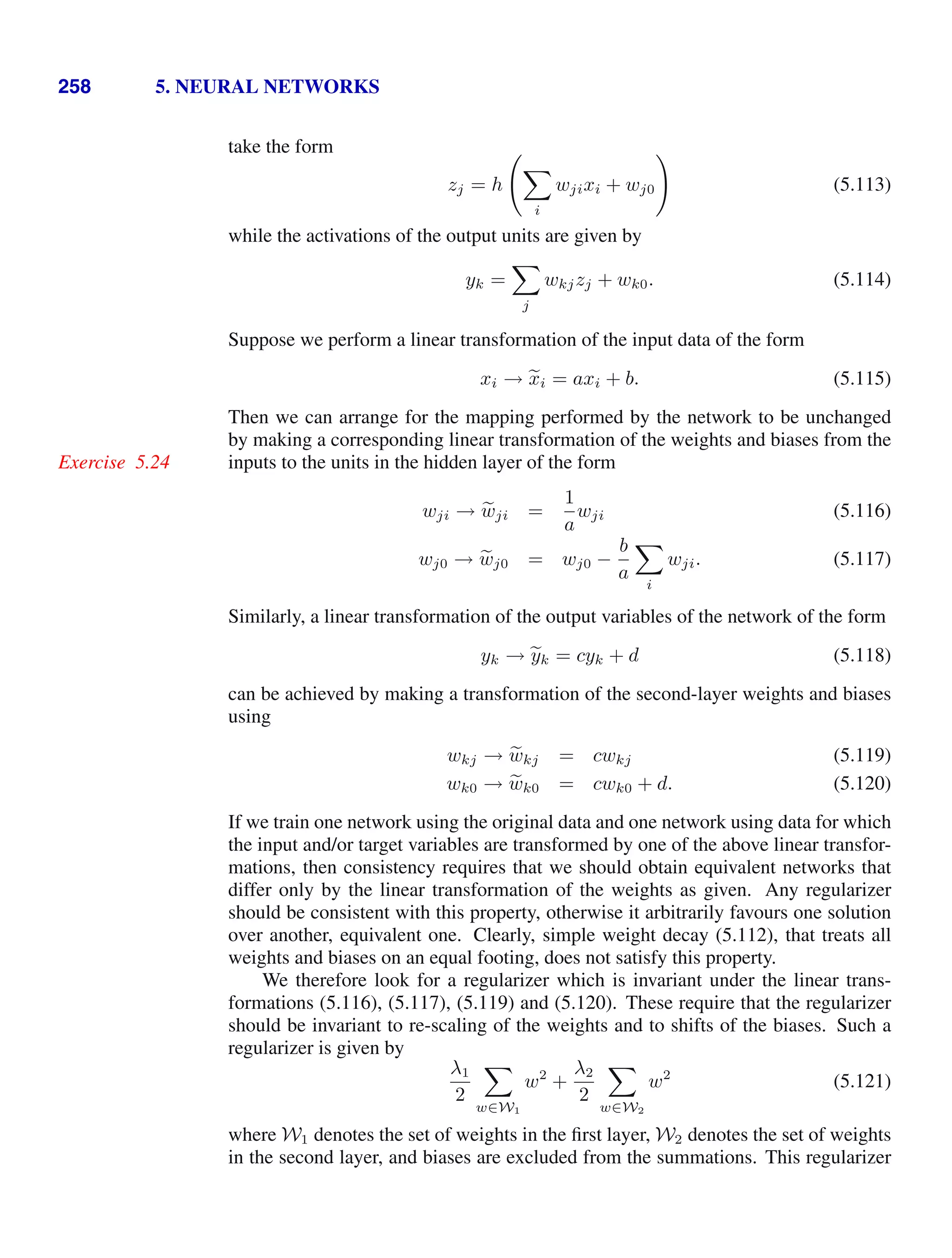
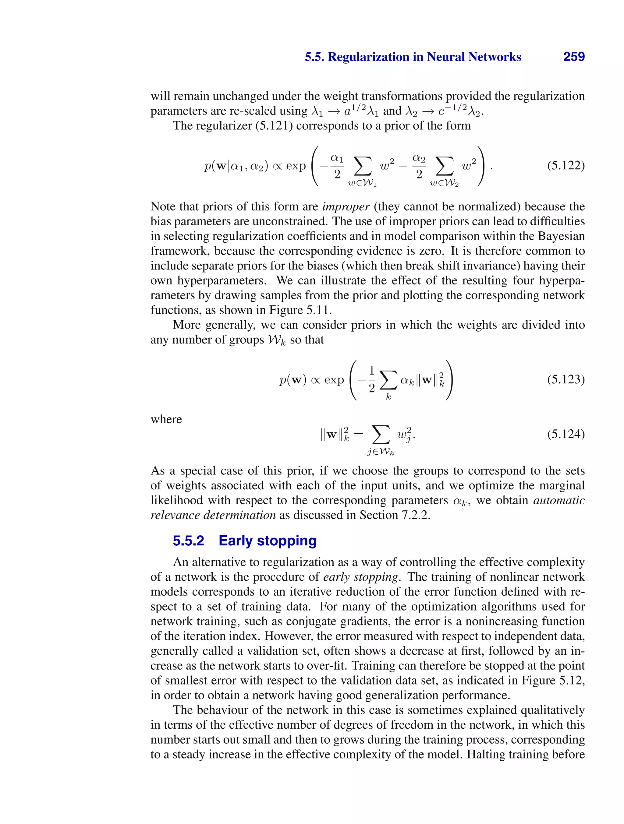
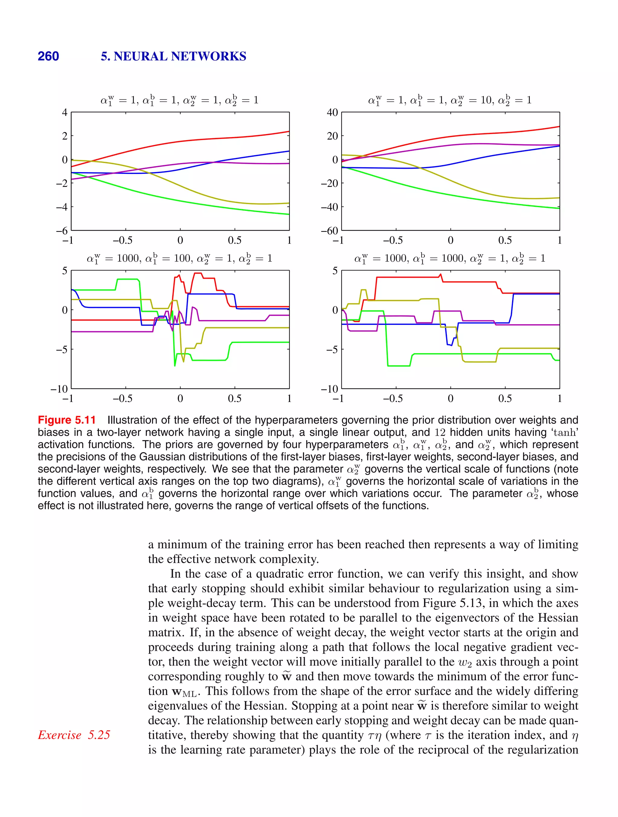
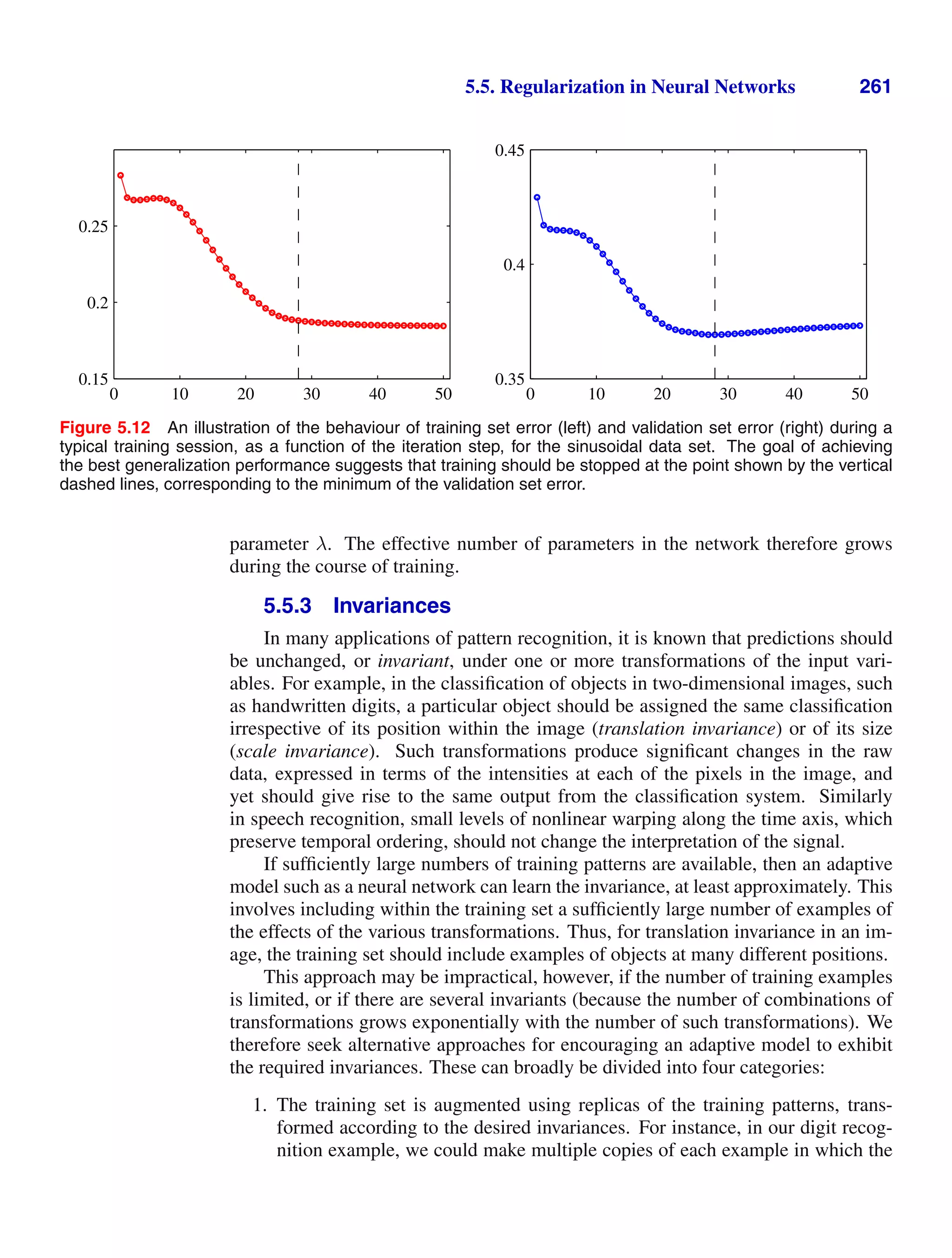
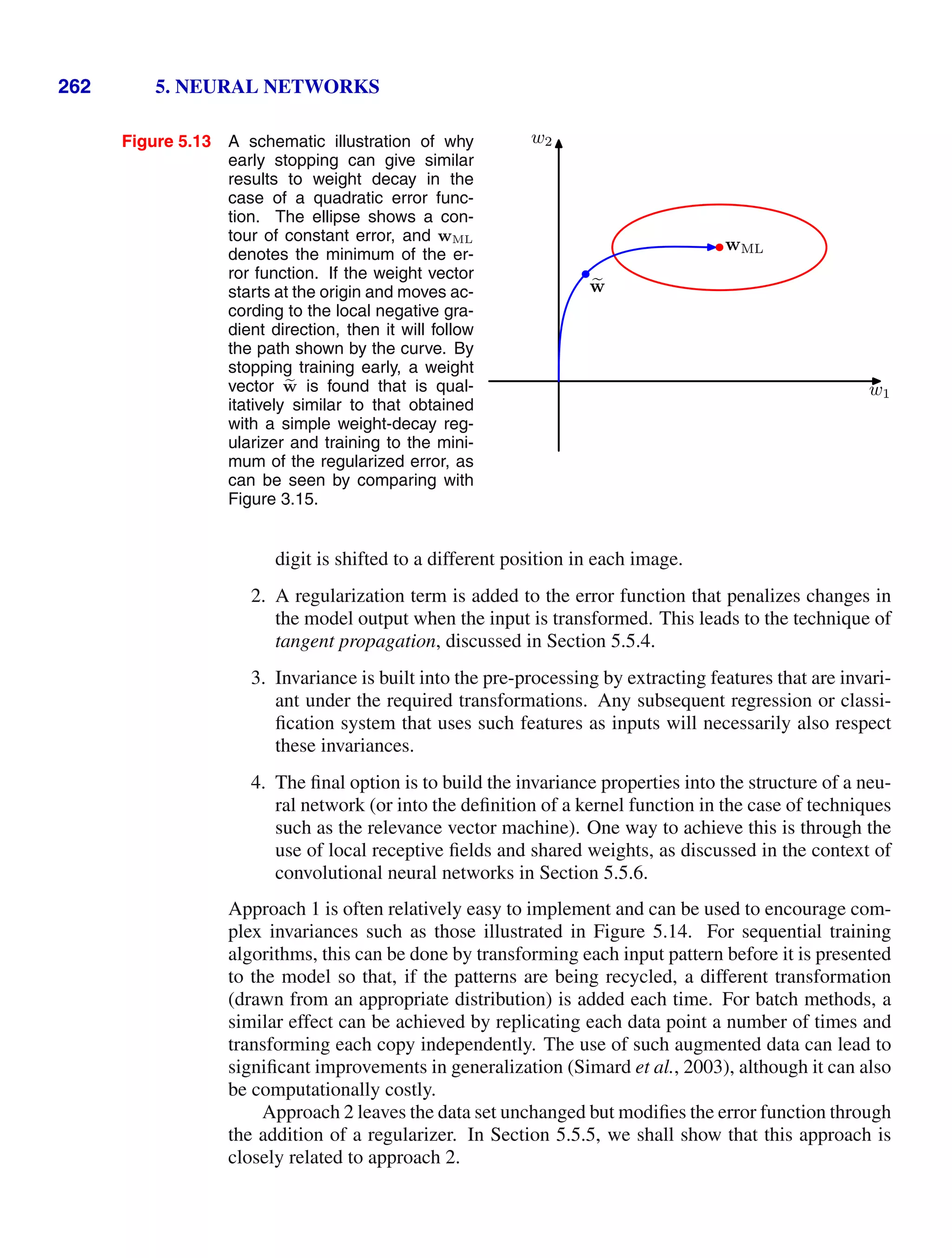
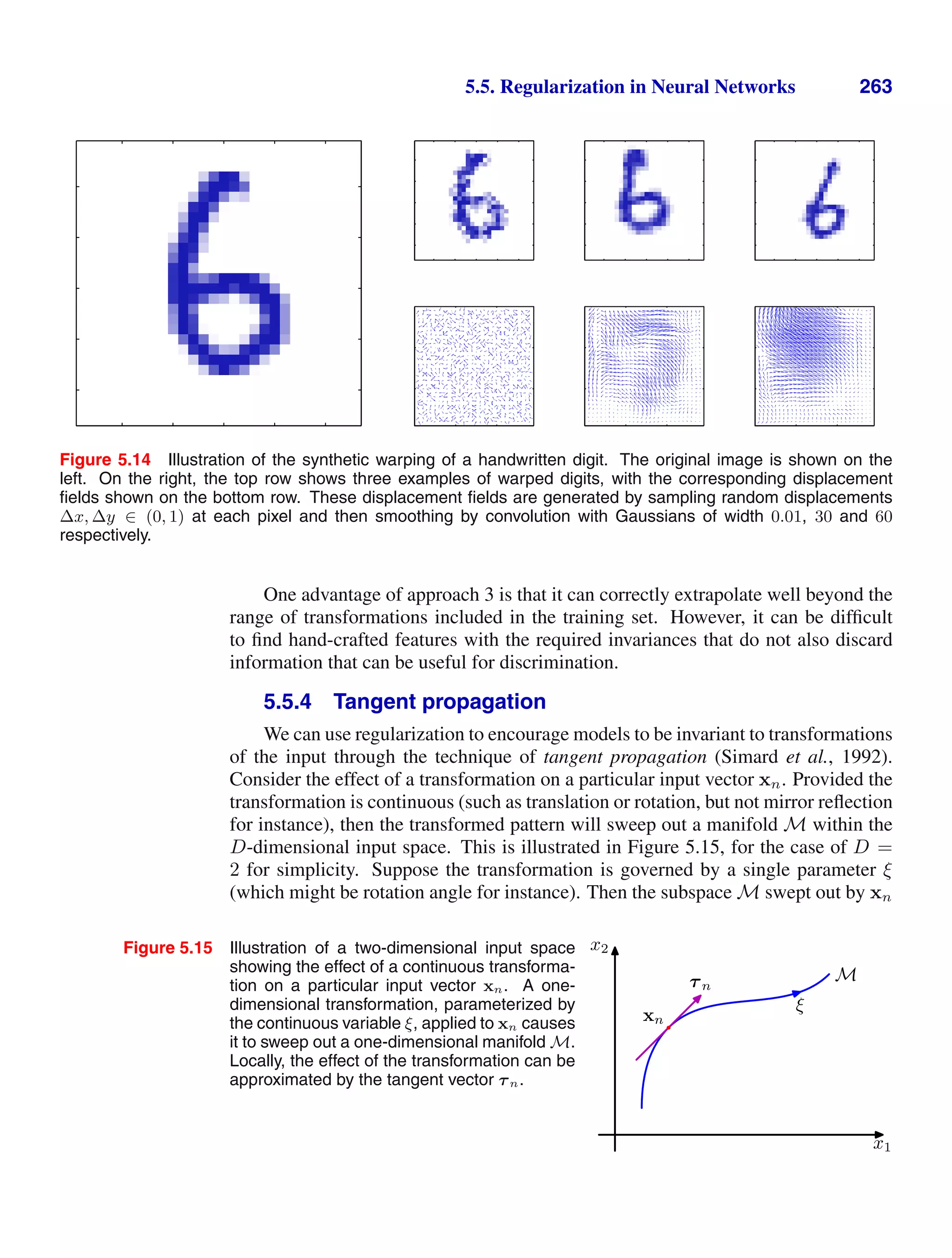
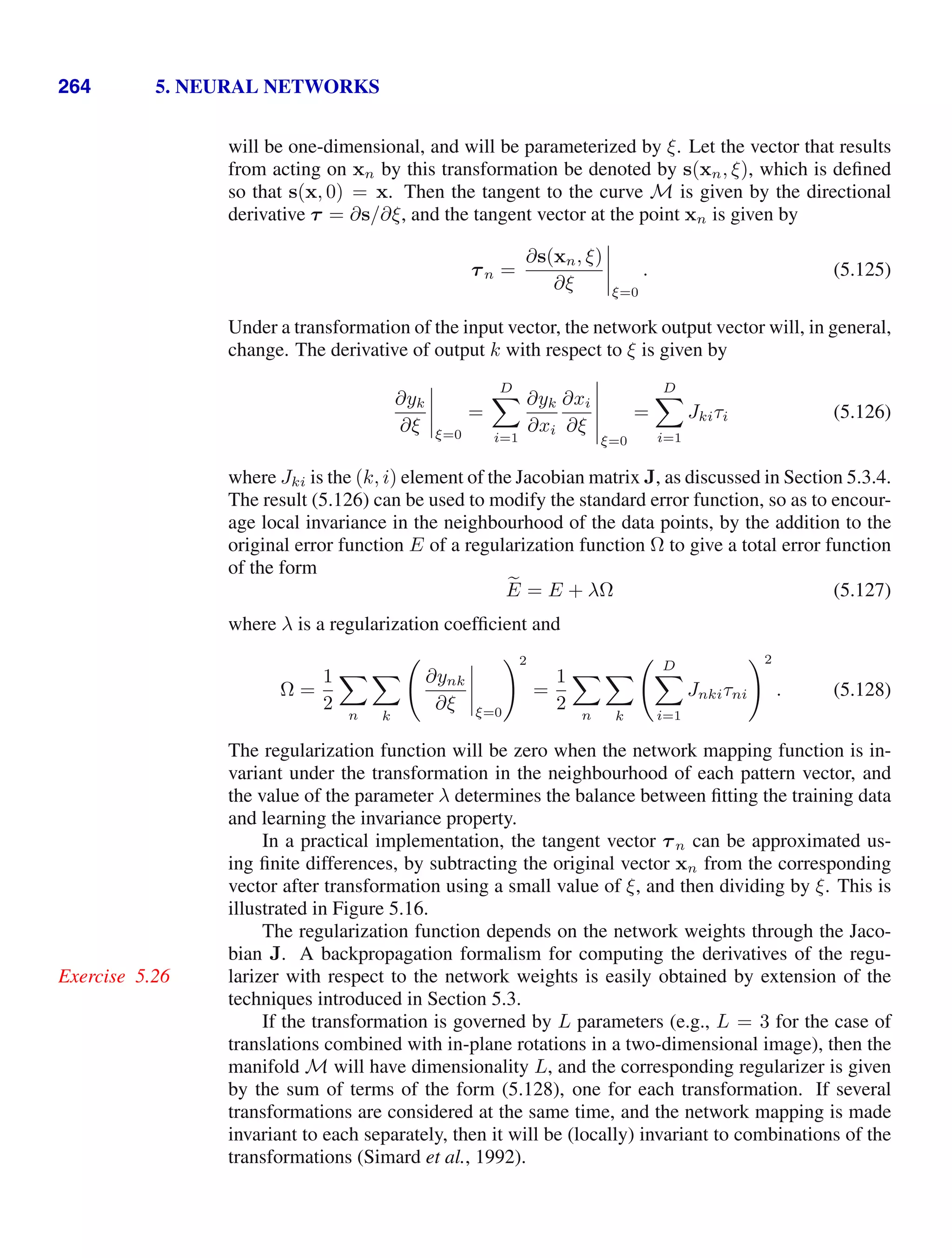
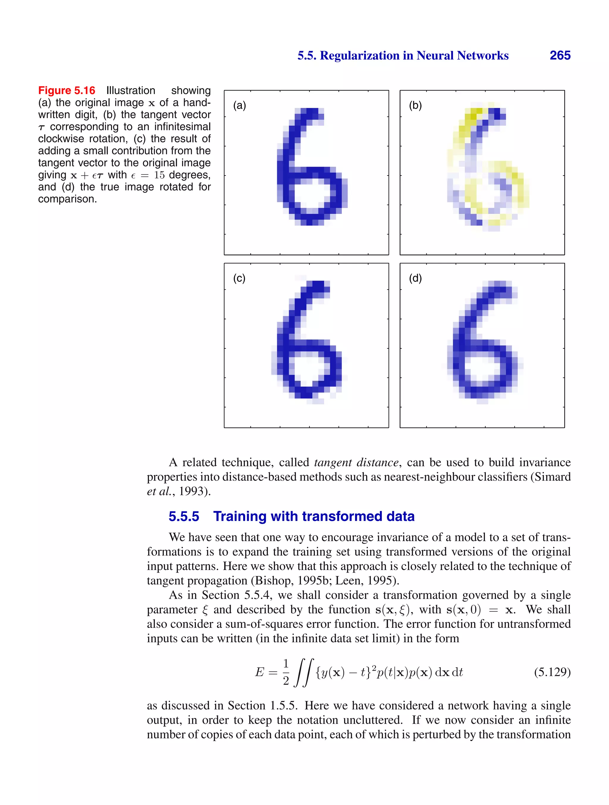
![266 5. NEURAL NETWORKS
in which the parameter ξ is drawn from a distribution p(ξ), then the error function
defined over this expanded data set can be written as
E =
1
2
{y(s(x, ξ)) − t}2
p(t|x)p(x)p(ξ) dx dt dξ. (5.130)
We now assume that the distribution p(ξ) has zero mean with small variance, so that
we are only considering small transformations of the original input vectors. We can
then expand the transformation function as a Taylor series in powers of ξ to give
s(x, ξ) = s(x, 0) + ξ
∂
∂ξ
s(x, ξ)
ξ=0
+
ξ2
2
∂2
∂ξ2
s(x, ξ)
ξ=0
+ O(ξ3
)
= x + ξτ +
1
2
ξ2
τ
+ O(ξ3
)
where τ
denotes the second derivative of s(x, ξ) with respect to ξ evaluated at ξ = 0.
This allows us to expand the model function to give
y(s(x, ξ)) = y(x) + ξτT
∇y(x) +
ξ2
2
-
(τ
)
T
∇y(x) + τT
∇∇y(x)τ
.
+ O(ξ3
).
Substituting into the mean error function (5.130) and expanding, we then have
E =
1
2
{y(x) − t}2
p(t|x)p(x) dx dt
+ E[ξ]
{y(x) − t}τT
∇y(x)p(t|x)p(x) dx dt
+ E[ξ2
]
{y(x) − t}
1
2
(τ
)
T
∇y(x) + τT
∇∇y(x)τ
+ τT
∇y(x)
2
.
p(t|x)p(x) dx dt + O(ξ3
).
Because the distribution of transformations has zero mean we have E[ξ] = 0. Also,
we shall denote E[ξ2
] by λ. Omitting terms of O(ξ3
), the average error function then
becomes
E = E + λΩ (5.131)
where E is the original sum-of-squares error, and the regularization term Ω takes the
form
Ω =
{y(x) − E[t|x]}
1
2
(τ
)
T
∇y(x) + τT
∇∇y(x)τ
+ τT
∇y(x)
2
p(x) dx (5.132)
in which we have performed the integration over t.](https://image.slidesharecdn.com/bishop-patternrecognitionandmachinelearning-230316082240-9af1cdaa/75/Bishop-Pattern-Recognition-and-Machine-Learning-pdf-283-2048.jpg)
![5.5. Regularization in Neural Networks 267
We can further simplify this regularization term as follows. In Section 1.5.5 we
saw that the function that minimizes the sum-of-squares error is given by the condi-
tional average E[t|x] of the target values t. From (5.131) we see that the regularized
error will equal the unregularized sum-of-squares plus terms which are O(ξ), and so
the network function that minimizes the total error will have the form
y(x) = E[t|x] + O(ξ). (5.133)
Thus, to leading order in ξ, the first term in the regularizer vanishes and we are left
with
Ω =
1
2
τT
∇y(x)
2
p(x) dx (5.134)
which is equivalent to the tangent propagation regularizer (5.128).
If we consider the special case in which the transformation of the inputs simply
consists of the addition of random noise, so that x → x + ξ, then the regularizer
takes the form
Exercise 5.27
Ω =
1
2
∇y(x)
2
p(x) dx (5.135)
which is known as Tikhonov regularization (Tikhonov and Arsenin, 1977; Bishop,
1995b). Derivatives of this regularizer with respect to the network weights can be
found using an extended backpropagation algorithm (Bishop, 1993). We see that, for
small noise amplitudes, Tikhonov regularization is related to the addition of random
noise to the inputs, which has been shown to improve generalization in appropriate
circumstances (Sietsma and Dow, 1991).
5.5.6 Convolutional networks
Another approach to creating models that are invariant to certain transformation
of the inputs is to build the invariance properties into the structure of a neural net-
work. This is the basis for the convolutional neural network (Le Cun et al., 1989;
LeCun et al., 1998), which has been widely applied to image data.
Consider the specific task of recognizing handwritten digits. Each input image
comprises a set of pixel intensity values, and the desired output is a posterior proba-
bility distribution over the ten digit classes. We know that the identity of the digit is
invariant under translations and scaling as well as (small) rotations. Furthermore, the
network must also exhibit invariance to more subtle transformations such as elastic
deformations of the kind illustrated in Figure 5.14. One simple approach would be to
treat the image as the input to a fully connected network, such as the kind shown in
Figure 5.1. Given a sufficiently large training set, such a network could in principle
yield a good solution to this problem and would learn the appropriate invariances by
example.
However, this approach ignores a key property of images, which is that nearby
pixels are more strongly correlated than more distant pixels. Many of the modern
approaches to computer vision exploit this property by extracting local features that
depend only on small subregions of the image. Information from such features can
then be merged in later stages of processing in order to detect higher-order features](https://image.slidesharecdn.com/bishop-patternrecognitionandmachinelearning-230316082240-9af1cdaa/75/Bishop-Pattern-Recognition-and-Machine-Learning-pdf-284-2048.jpg)
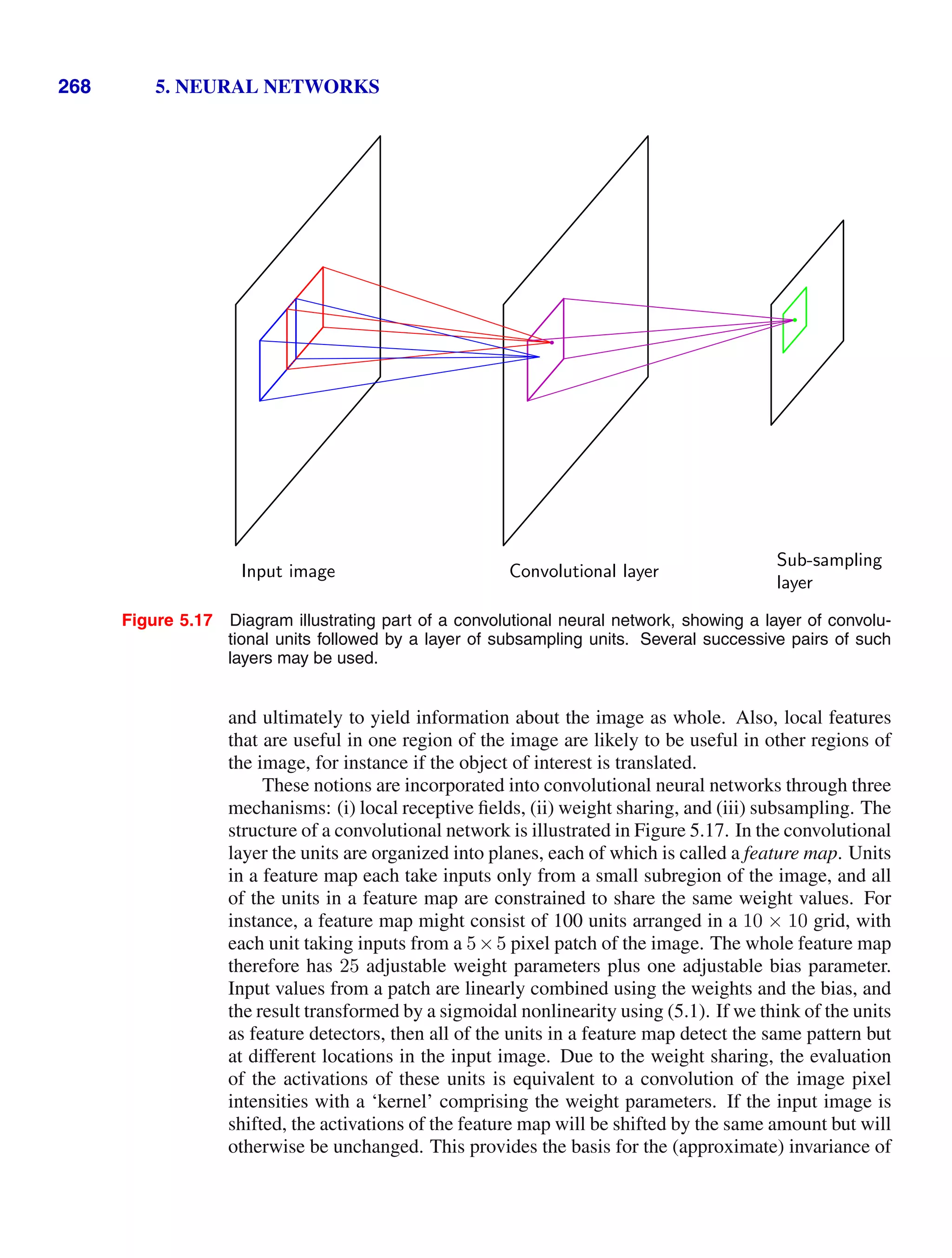
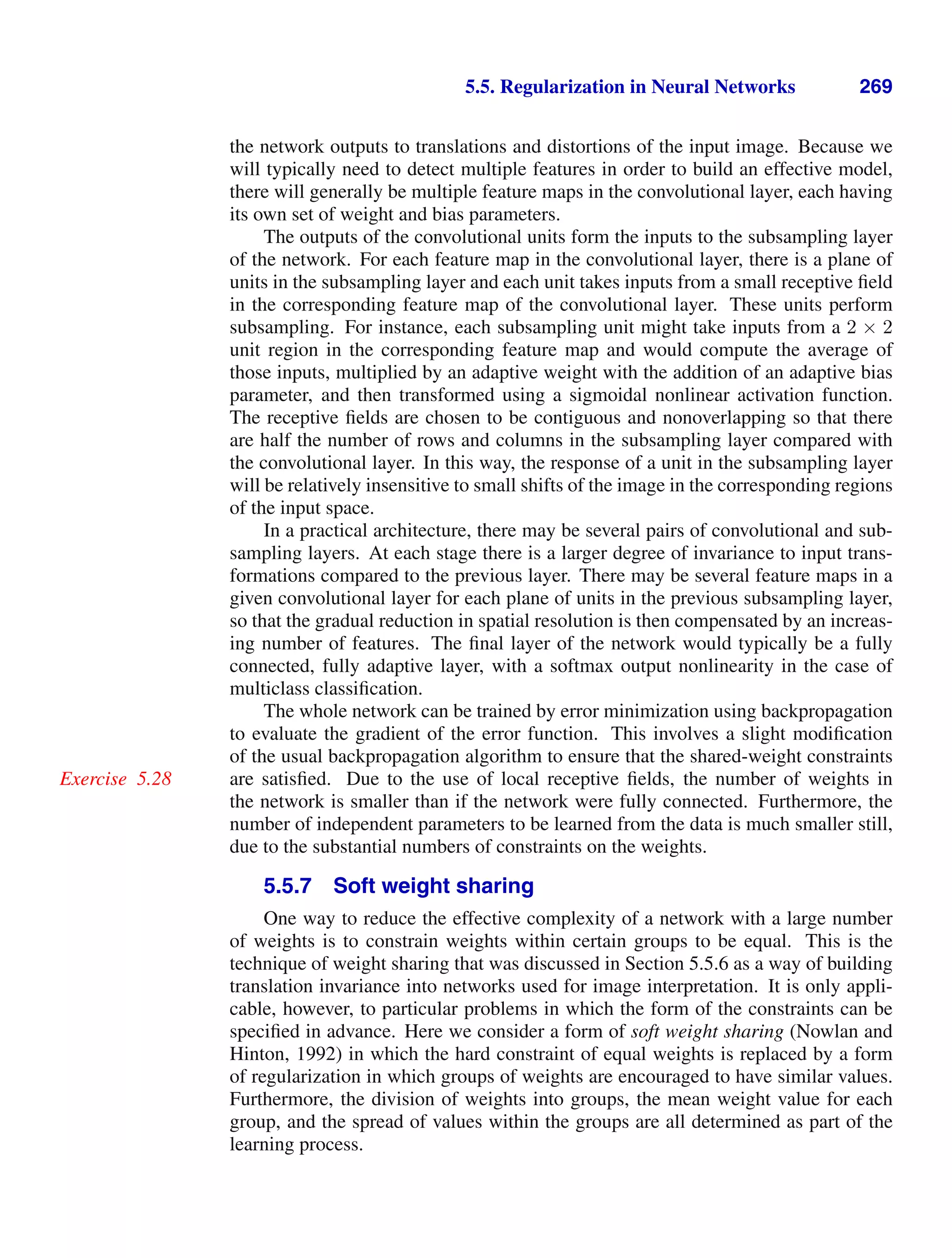
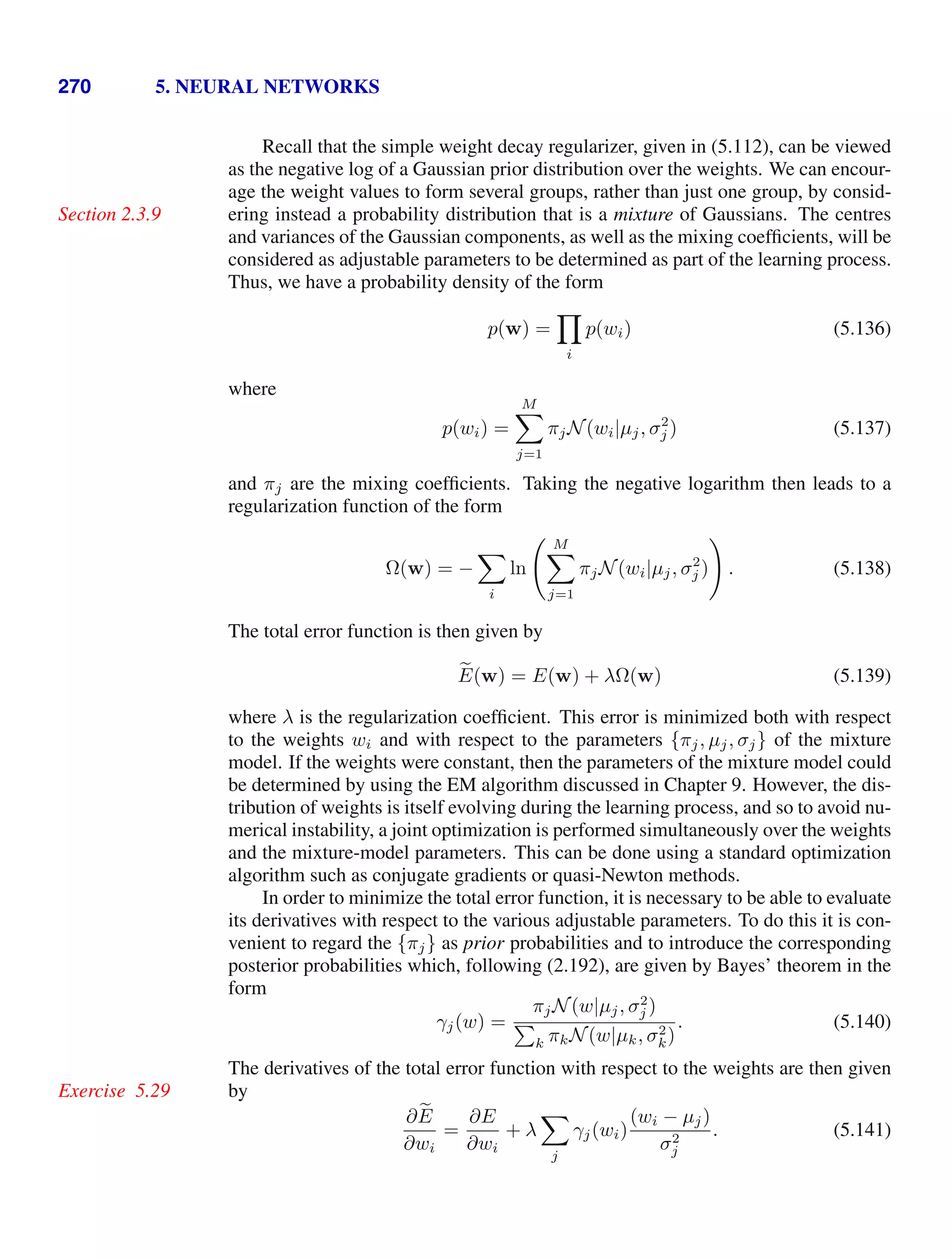
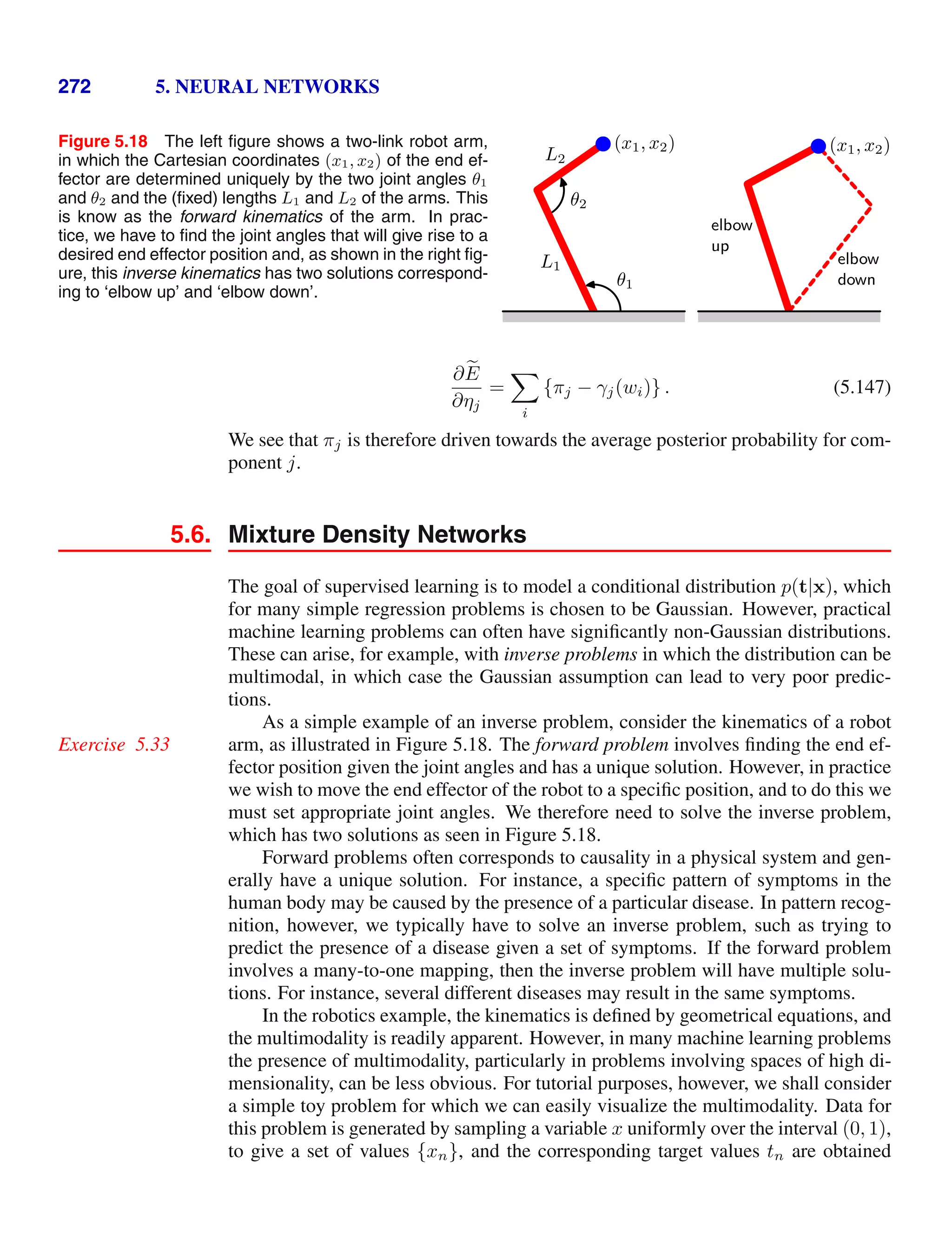
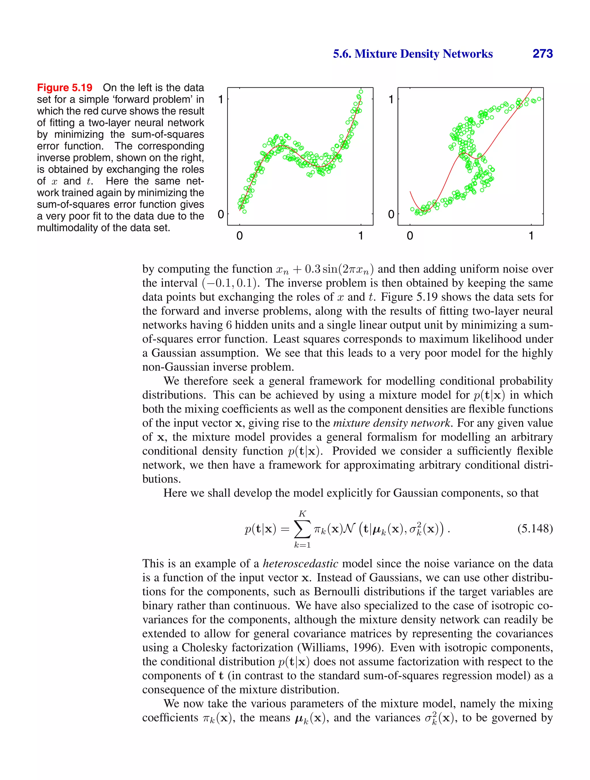
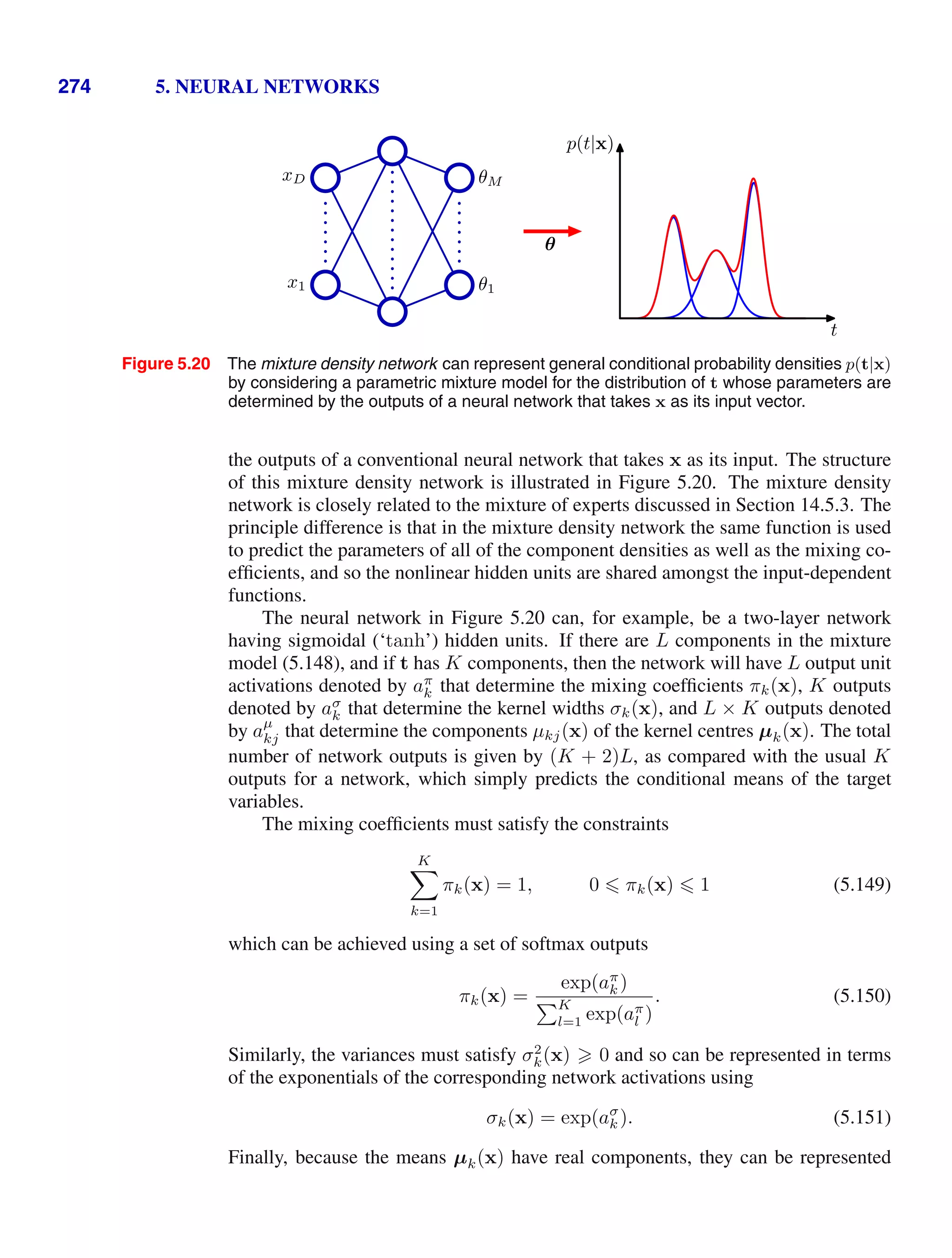
![276 5. NEURAL NETWORKS
Figure 5.21 (a) Plot of the mixing
coefficients πk(x) as a function of
x for the three kernel functions in a
mixture density network trained on
the data shown in Figure 5.19. The
model has three Gaussian compo-
nents, and uses a two-layer multi-
layer perceptron with five ‘tanh’ sig-
moidal units in the hidden layer, and
nine outputs (corresponding to the 3
means and 3 variances of the Gaus-
sian components and the 3 mixing
coefficients). At both small and large
values of x, where the conditional
probability density of the target data
is unimodal, only one of the ker-
nels has a high value for its prior
probability, while at intermediate val-
ues of x, where the conditional den-
sity is trimodal, the three mixing co-
efficients have comparable values.
(b) Plots of the means µk(x) using
the same colour coding as for the
mixing coefficients. (c) Plot of the
contours of the corresponding con-
ditional probability density of the tar-
get data for the same mixture den-
sity network. (d) Plot of the ap-
proximate conditional mode, shown
by the red points, of the conditional
density.
0 1
0
1
(a)
0 1
0
1
(b)
(c)
0 1
0
1
0 1
0
1
(d)
We illustrate the use of a mixture density network by returning to the toy ex-
ample of an inverse problem shown in Figure 5.19. Plots of the mixing coeffi-
cients πk(x), the means µk(x), and the conditional density contours corresponding
to p(t|x), are shown in Figure 5.21. The outputs of the neural network, and hence the
parameters in the mixture model, are necessarily continuous single-valued functions
of the input variables. However, we see from Figure 5.21(c) that the model is able to
produce a conditional density that is unimodal for some values of x and trimodal for
other values by modulating the amplitudes of the mixing components πk(x).
Once a mixture density network has been trained, it can predict the conditional
density function of the target data for any given value of the input vector. This
conditional density represents a complete description of the generator of the data, so
far as the problem of predicting the value of the output vector is concerned. From
this density function we can calculate more specific quantities that may be of interest
in different applications. One of the simplest of these is the mean, corresponding to
the conditional average of the target data, and is given by
E [t|x] =
tp(t|x) dt =
K
k=1
πk(x)µk(x) (5.158)](https://image.slidesharecdn.com/bishop-patternrecognitionandmachinelearning-230316082240-9af1cdaa/75/Bishop-Pattern-Recognition-and-Machine-Learning-pdf-293-2048.jpg)
![5.7. Bayesian Neural Networks 277
where we have used (5.148). Because a standard network trained by least squares
is approximating the conditional mean, we see that a mixture density network can
reproduce the conventional least-squares result as a special case. Of course, as we
have already noted, for a multimodal distribution the conditional mean is of limited
value.
We can similarly evaluate the variance of the density function about the condi-
tional average, to give
Exercise 5.37
s2
(x) = E
t − E[t|x]
2
|x (5.159)
=
K
k=1
πk(x)
⎧
⎨
⎩
σ2
k(x) +
'
'
'
'
'
µk(x) −
K
l=1
πl(x)µl(x)
'
'
'
'
'
2
⎫
⎬
⎭
(5.160)
where we have used (5.148) and (5.158). This is more general than the corresponding
least-squares result because the variance is a function of x.
We have seen that for multimodal distributions, the conditional mean can give
a poor representation of the data. For instance, in controlling the simple robot arm
shown in Figure 5.18, we need to pick one of the two possible joint angle settings
in order to achieve the desired end-effector location, whereas the average of the two
solutions is not itself a solution. In such cases, the conditional mode may be of
more value. Because the conditional mode for the mixture density network does not
have a simple analytical solution, this would require numerical iteration. A simple
alternative is to take the mean of the most probable component (i.e., the one with the
largest mixing coefficient) at each value of x. This is shown for the toy data set in
Figure 5.21(d).
5.7. Bayesian Neural Networks
So far, our discussion of neural networks has focussed on the use of maximum like-
lihood to determine the network parameters (weights and biases). Regularized max-
imum likelihood can be interpreted as a MAP (maximum posterior) approach in
which the regularizer can be viewed as the logarithm of a prior parameter distribu-
tion. However, in a Bayesian treatment we need to marginalize over the distribution
of parameters in order to make predictions.
In Section 3.3, we developed a Bayesian solution for a simple linear regression
model under the assumption of Gaussian noise. We saw that the posterior distribu-
tion, which is Gaussian, could be evaluated exactly and that the predictive distribu-
tion could also be found in closed form. In the case of a multilayered network, the
highly nonlinear dependence of the network function on the parameter values means
that an exact Bayesian treatment can no longer be found. In fact, the log of the pos-
terior distribution will be nonconvex, corresponding to the multiple local minima in
the error function.
The technique of variational inference, to be discussed in Chapter 10, has been
applied to Bayesian neural networks using a factorized Gaussian approximation](https://image.slidesharecdn.com/bishop-patternrecognitionandmachinelearning-230316082240-9af1cdaa/75/Bishop-Pattern-Recognition-and-Machine-Learning-pdf-294-2048.jpg)
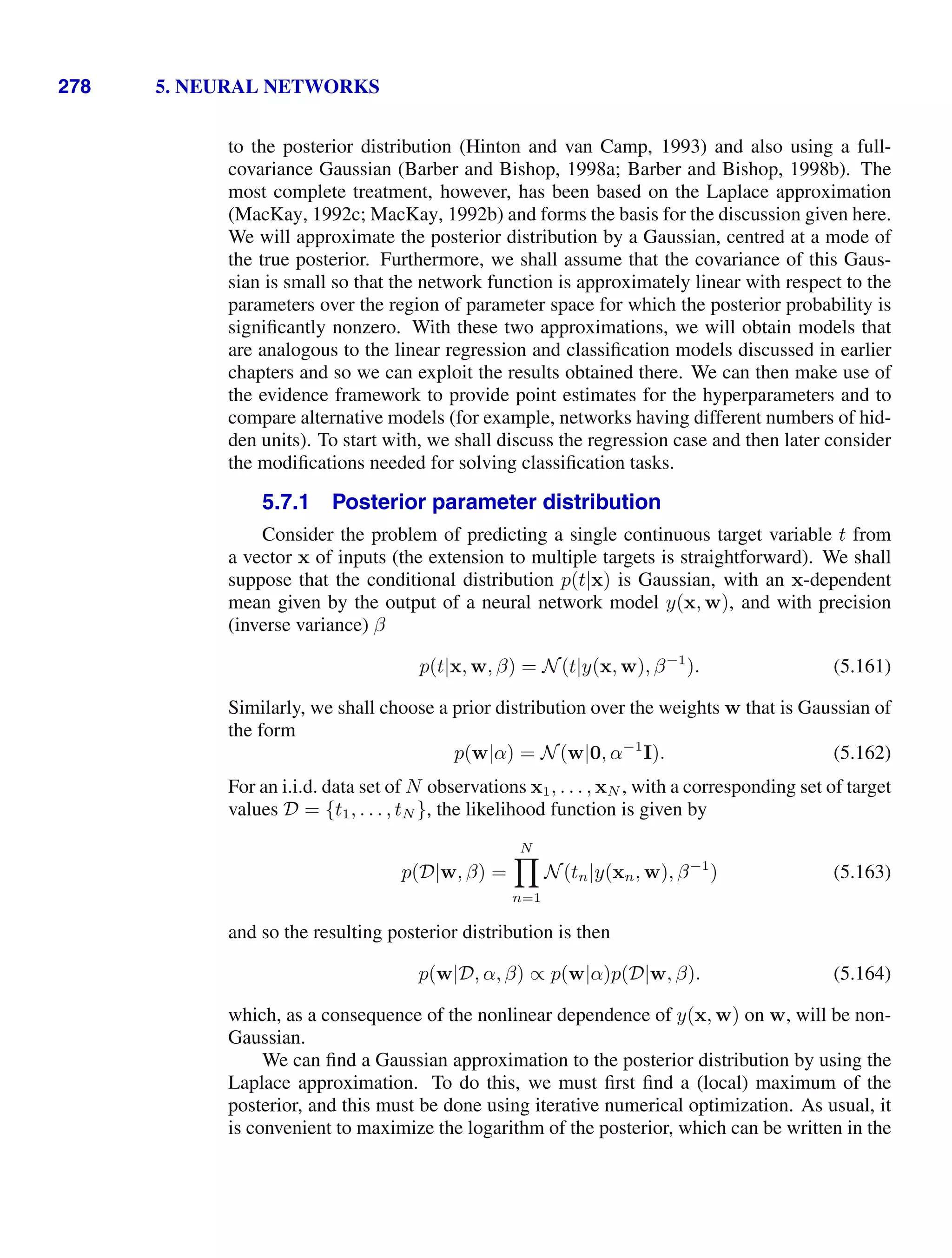
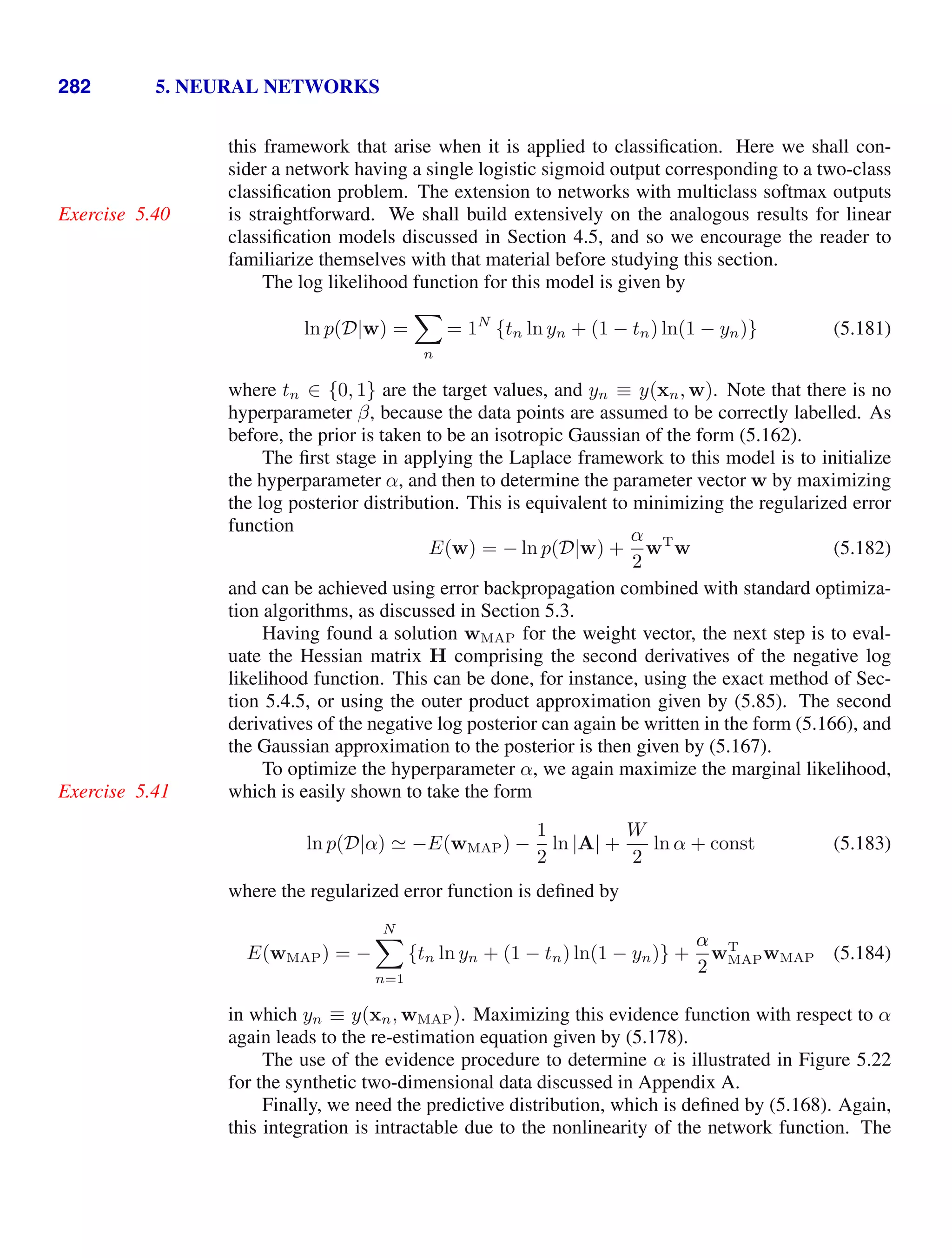
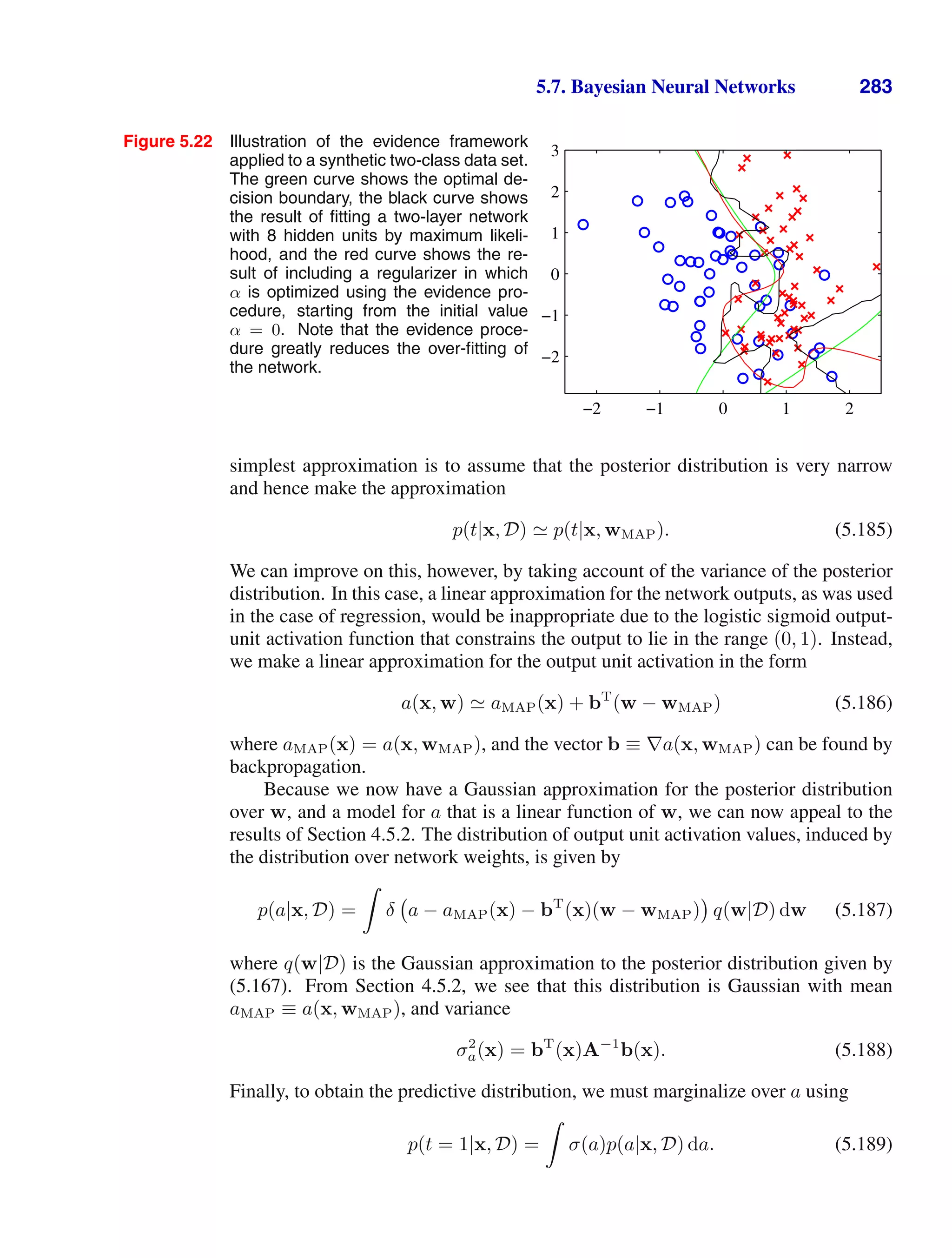
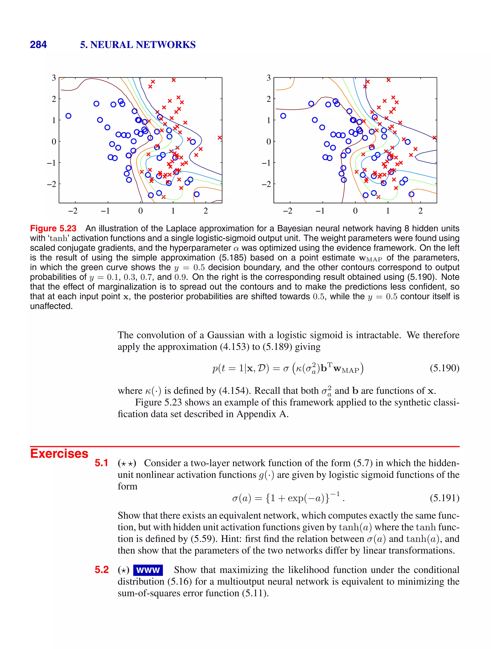

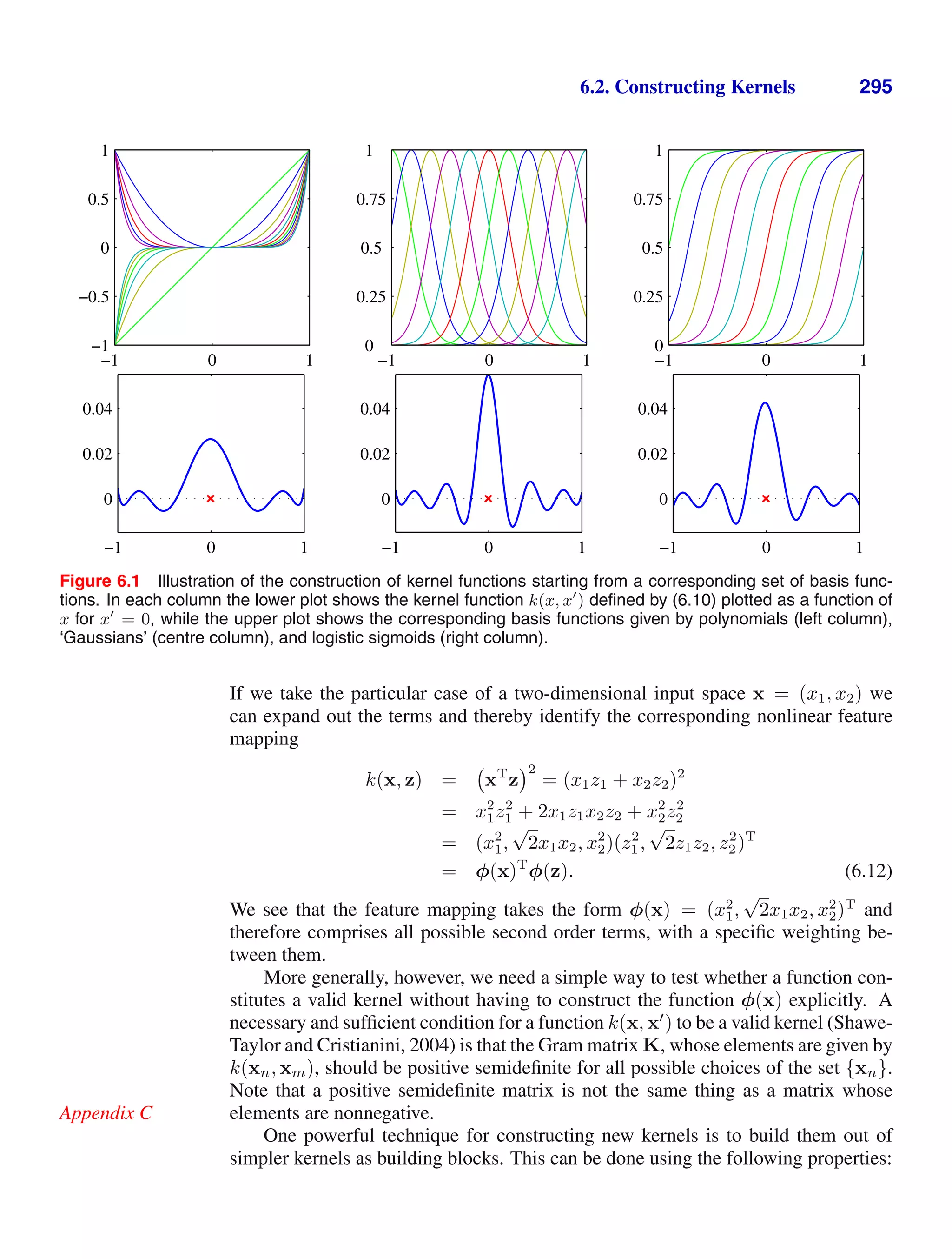
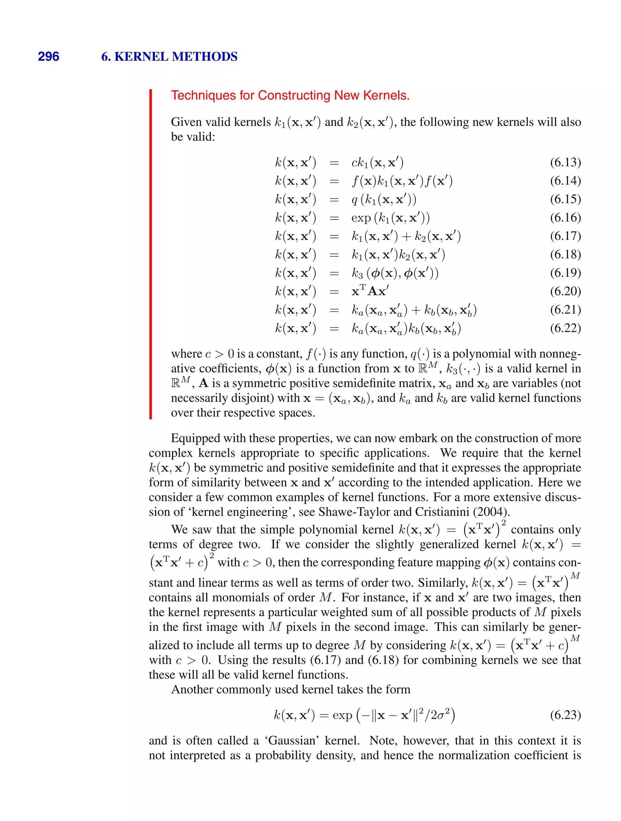
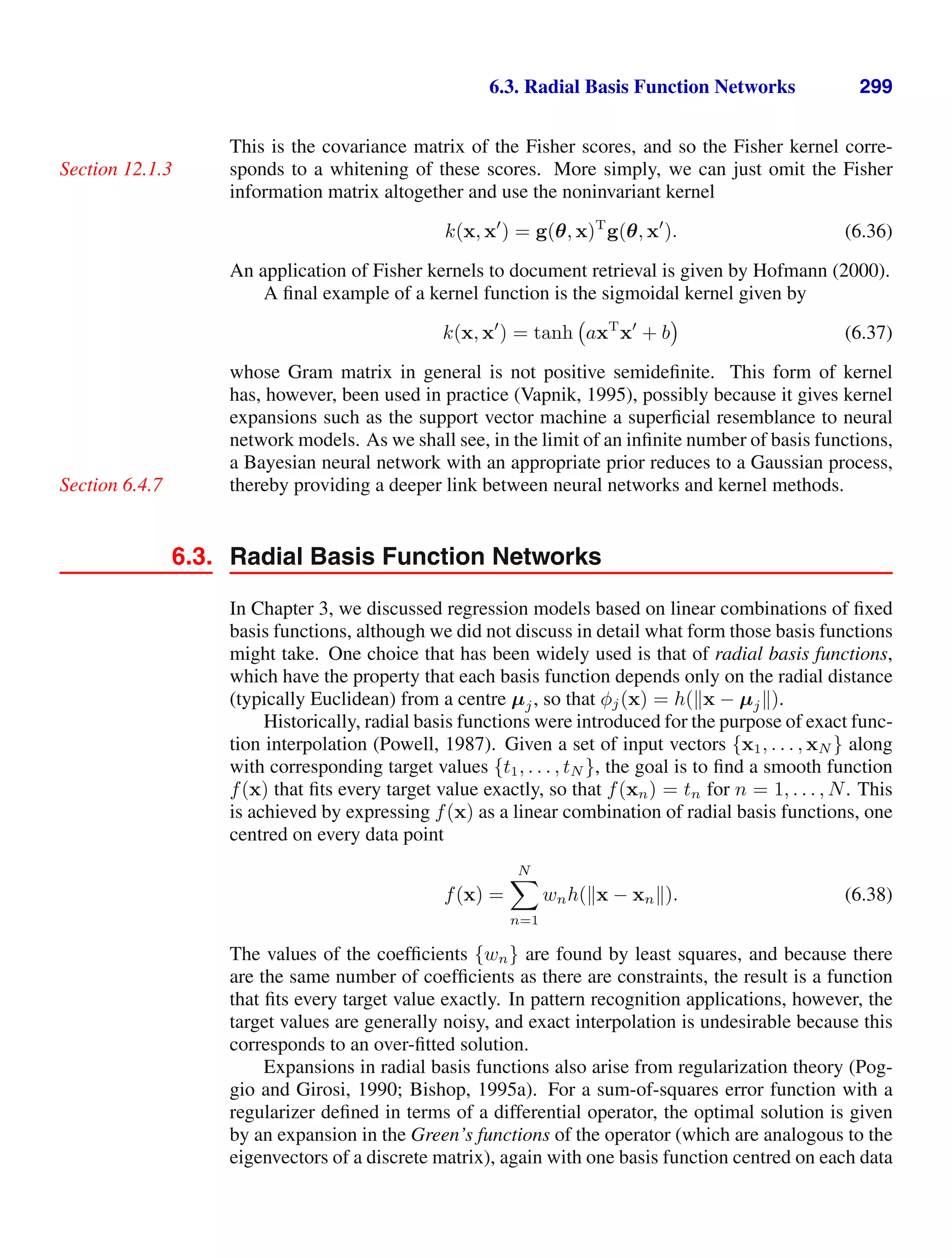
![302 6. KERNEL METHODS
the input variable, which is given by
y(x) = E[t|x] =
∞
−∞
tp(t|x) dt
=
tp(x, t) dt
p(x, t) dt
=
n
tf(x − xn, t − tn) dt
m
f(x − xm, t − tm) dt
. (6.43)
We now assume for simplicity that the component density functions have zero mean
so that ∞
−∞
f(x, t)t dt = 0 (6.44)
for all values of x. Using a simple change of variable, we then obtain
y(x) =
n
g(x − xn)tn
m
g(x − xm)
=
n
k(x, xn)tn (6.45)
where n, m = 1, . . . , N and the kernel function k(x, xn) is given by
k(x, xn) =
g(x − xn)
m
g(x − xm)
(6.46)
and we have defined
g(x) =
∞
−∞
f(x, t) dt. (6.47)
The result (6.45) is known as the Nadaraya-Watson model, or kernel regression
(Nadaraya, 1964; Watson, 1964). For a localized kernel function, it has the prop-
erty of giving more weight to the data points xn that are close to x. Note that the
kernel (6.46) satisfies the summation constraint
N
n=1
k(x, xn) = 1.](https://image.slidesharecdn.com/bishop-patternrecognitionandmachinelearning-230316082240-9af1cdaa/75/Bishop-Pattern-Recognition-and-Machine-Learning-pdf-319-2048.jpg)
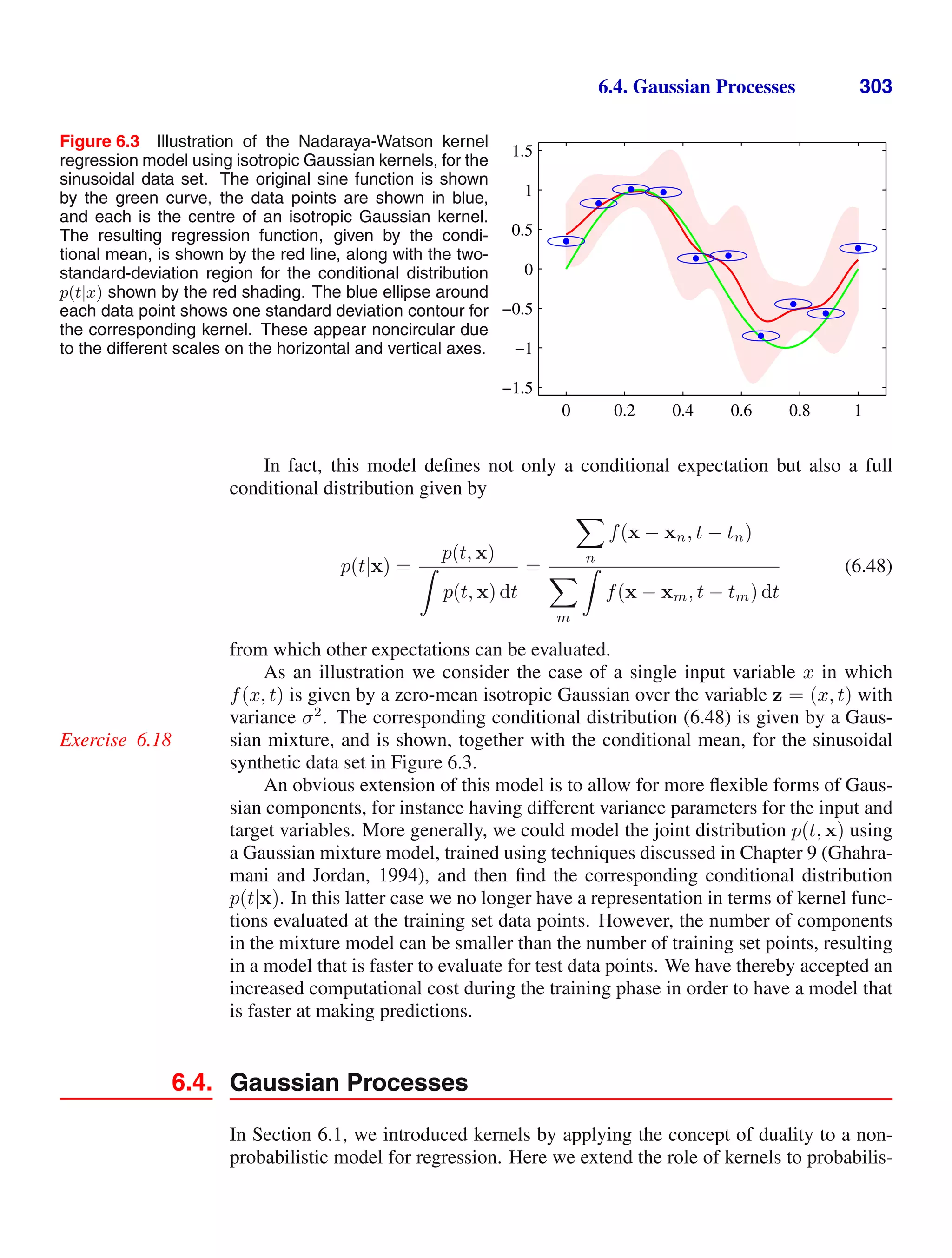
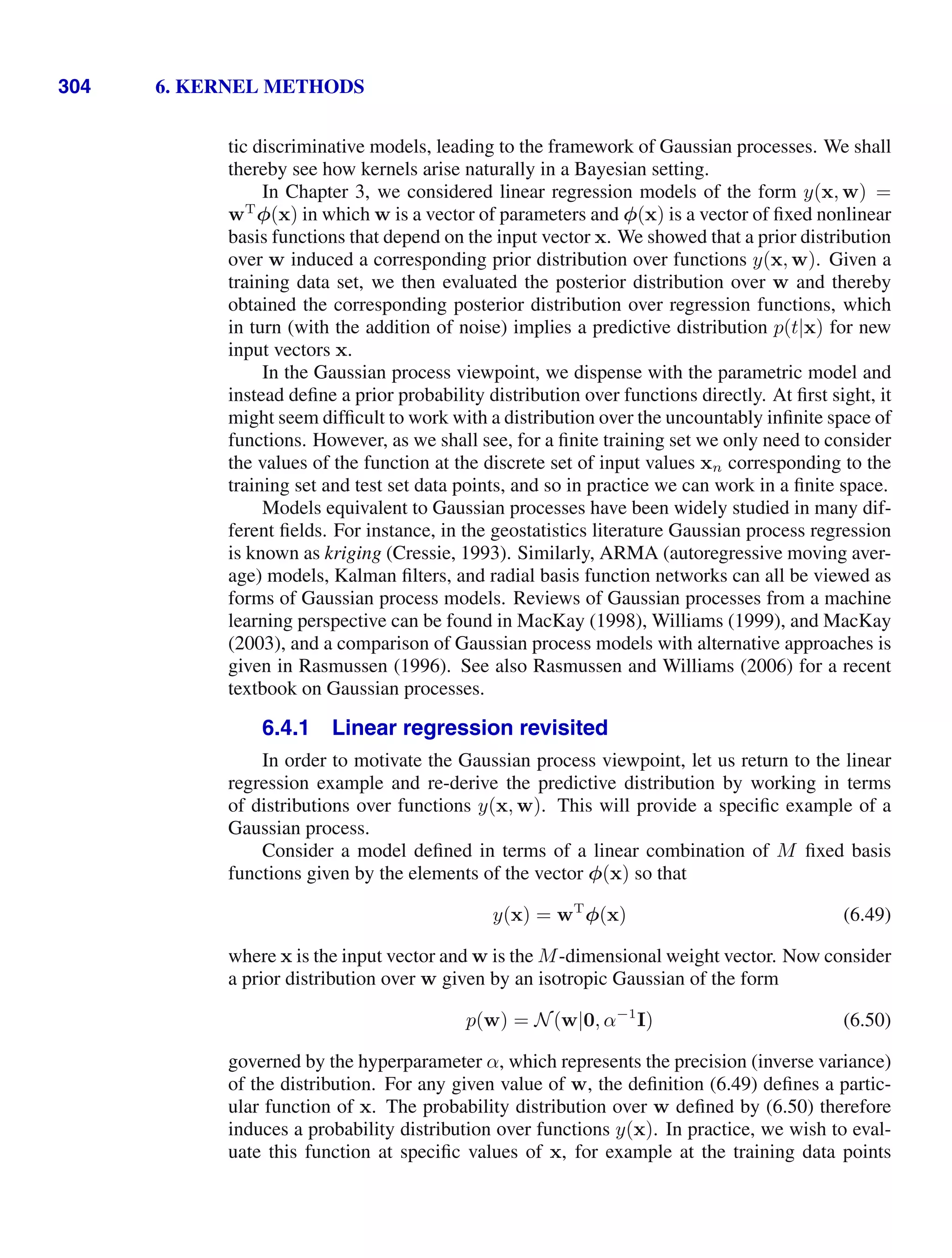
![6.4. Gaussian Processes 305
x1, . . . , xN . We are therefore interested in the joint distribution of the function val-
ues y(x1), . . . , y(xN ), which we denote by the vector y with elements yn = y(xn)
for n = 1, . . . , N. From (6.49), this vector is given by
y = Φw (6.51)
where Φ is the design matrix with elements Φnk = φk(xn). We can find the proba-
bility distribution of y as follows. First of all we note that y is a linear combination of
Gaussian distributed variables given by the elements of w and hence is itself Gaus-
sian. We therefore need only to find its mean and covariance, which are given from
Exercise 2.31
(6.50) by
E[y] = ΦE[w] = 0 (6.52)
cov[y] = E
yyT
= ΦE
wwT
ΦT
=
1
α
ΦΦT
= K (6.53)
where K is the Gram matrix with elements
Knm = k(xn, xm) =
1
α
φ(xn)T
φ(xm) (6.54)
and k(x, x
) is the kernel function.
This model provides us with a particular example of a Gaussian process. In gen-
eral, a Gaussian process is defined as a probability distribution over functions y(x)
such that the set of values of y(x) evaluated at an arbitrary set of points x1, . . . , xN
jointly have a Gaussian distribution. In cases where the input vector x is two di-
mensional, this may also be known as a Gaussian random field. More generally, a
stochastic process y(x) is specified by giving the joint probability distribution for
any finite set of values y(x1), . . . , y(xN ) in a consistent manner.
A key point about Gaussian stochastic processes is that the joint distribution
over N variables y1, . . . , yN is specified completely by the second-order statistics,
namely the mean and the covariance. In most applications, we will not have any
prior knowledge about the mean of y(x) and so by symmetry we take it to be zero.
This is equivalent to choosing the mean of the prior over weight values p(w|α) to
be zero in the basis function viewpoint. The specification of the Gaussian process is
then completed by giving the covariance of y(x) evaluated at any two values of x,
which is given by the kernel function
E [y(xn)y(xm)] = k(xn, xm). (6.55)
For the specific case of a Gaussian process defined by the linear regression model
(6.49) with a weight prior (6.50), the kernel function is given by (6.54).
We can also define the kernel function directly, rather than indirectly through a
choice of basis function. Figure 6.4 shows samples of functions drawn from Gaus-
sian processes for two different choices of kernel function. The first of these is a
‘Gaussian’ kernel of the form (6.23), and the second is the exponential kernel given
by
k(x, x
) = exp (−θ |x − x
|) (6.56)
which corresponds to the Ornstein-Uhlenbeck process originally introduced by Uh-
lenbeck and Ornstein (1930) to describe Brownian motion.](https://image.slidesharecdn.com/bishop-patternrecognitionandmachinelearning-230316082240-9af1cdaa/75/Bishop-Pattern-Recognition-and-Machine-Learning-pdf-322-2048.jpg)
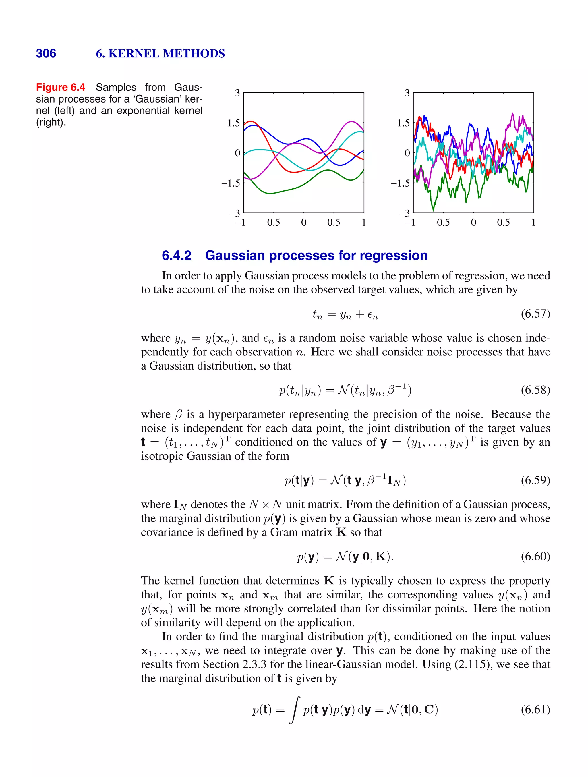
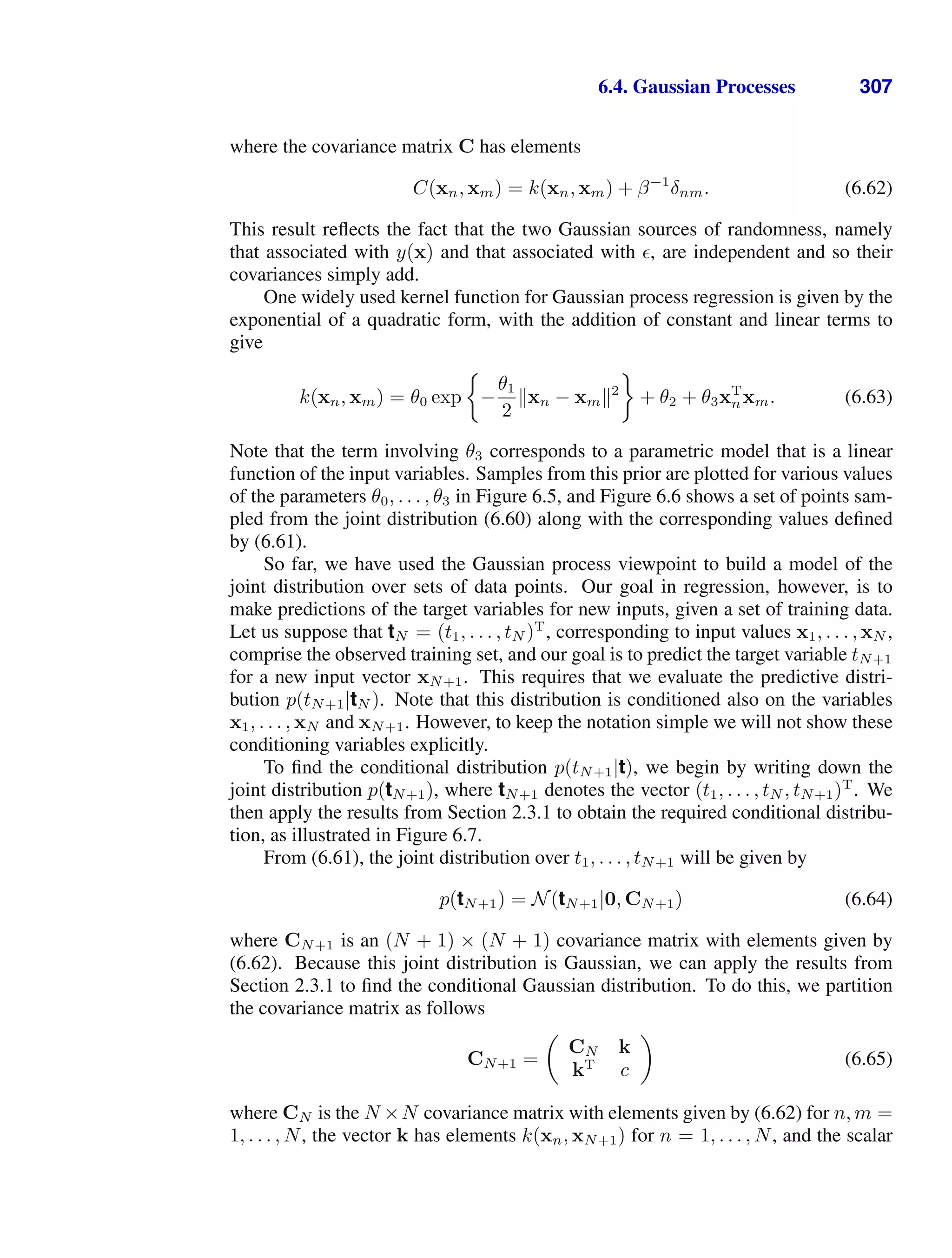
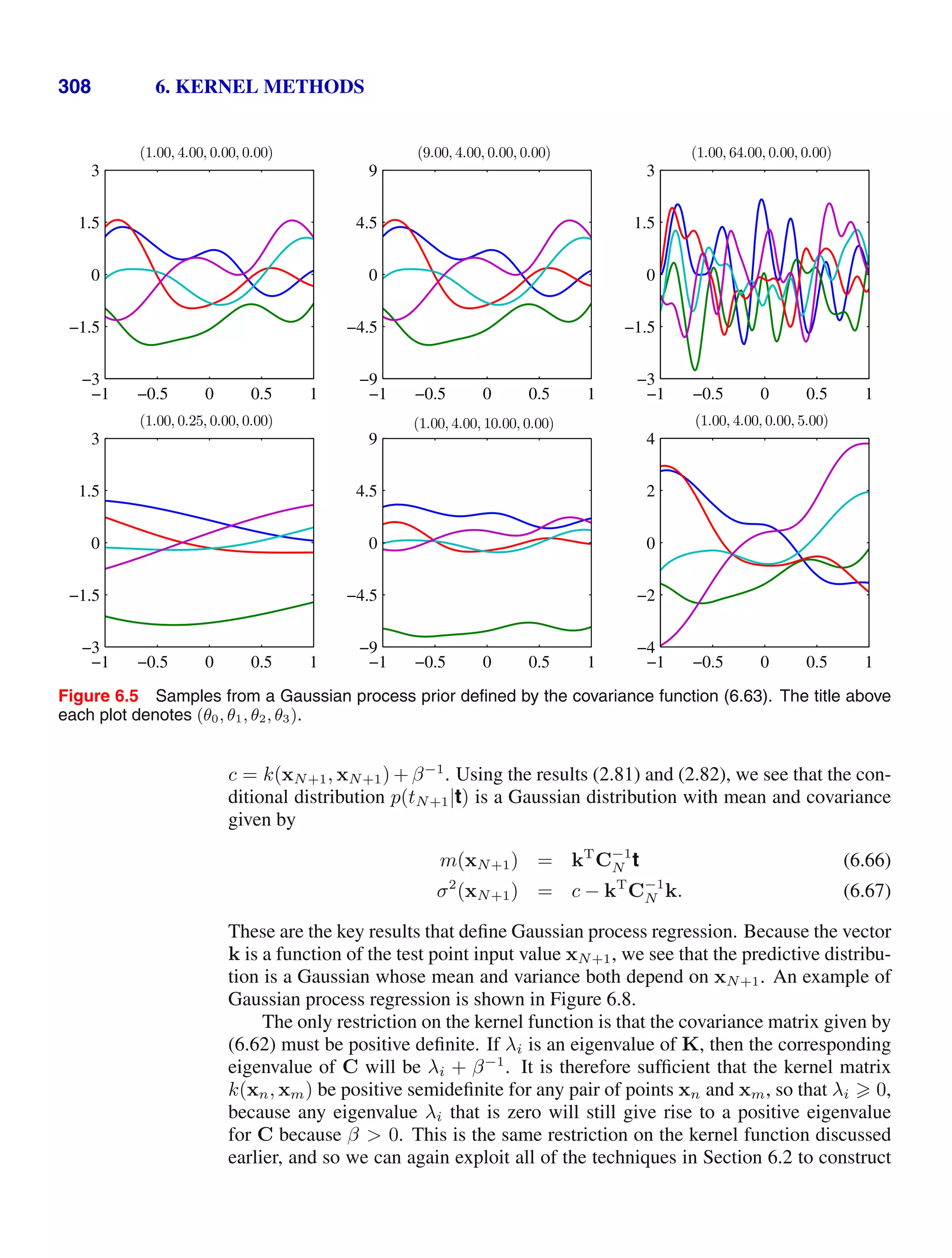
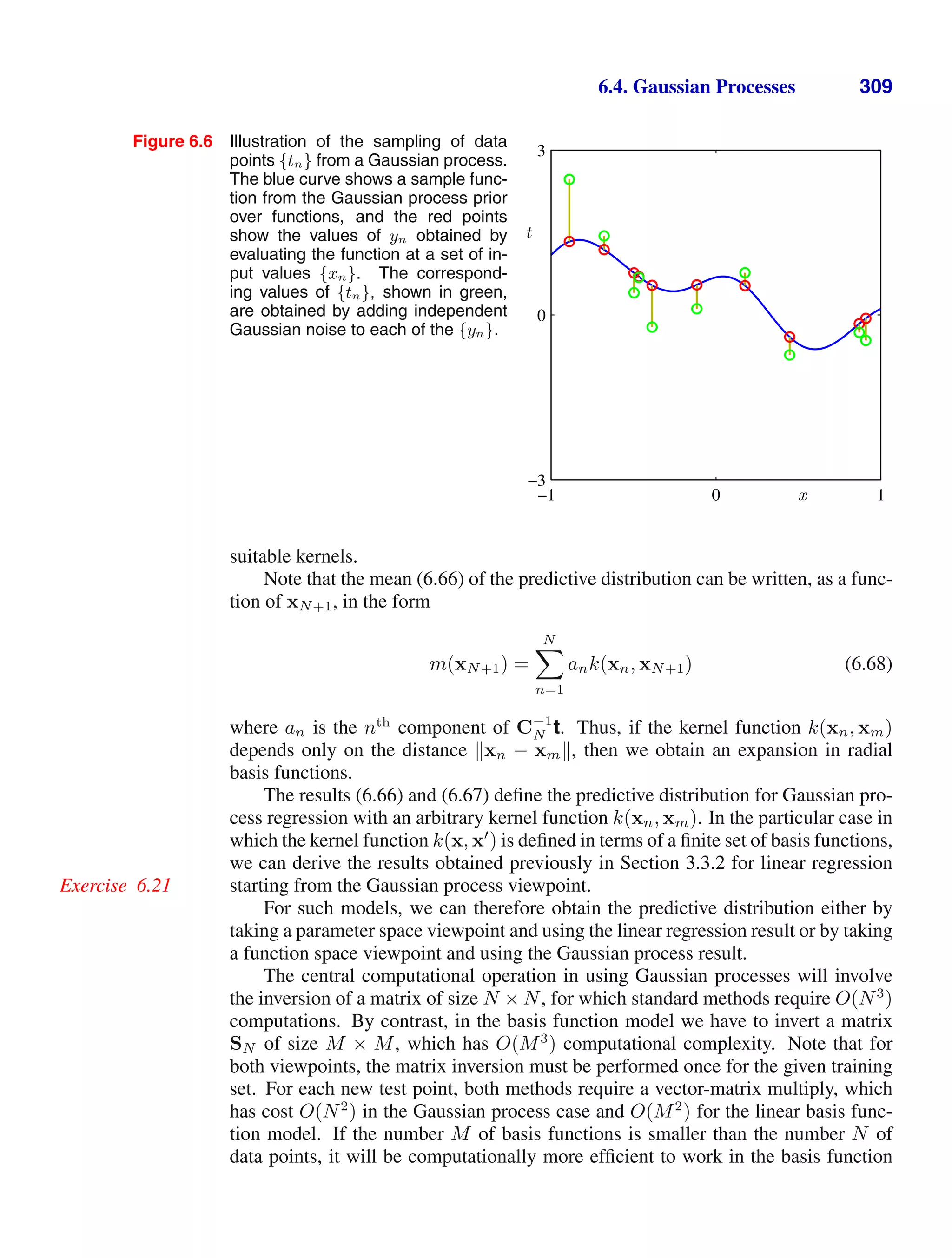
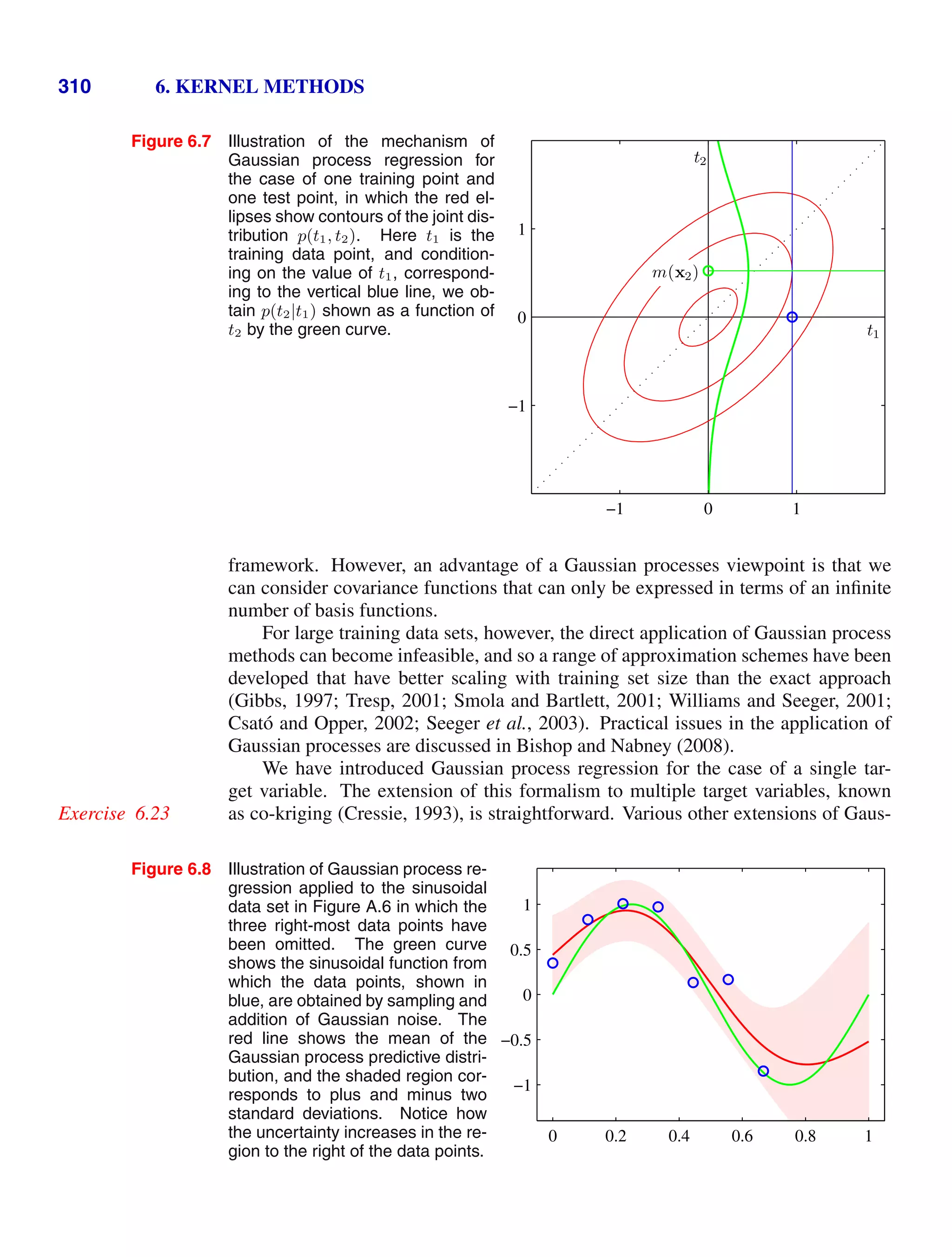
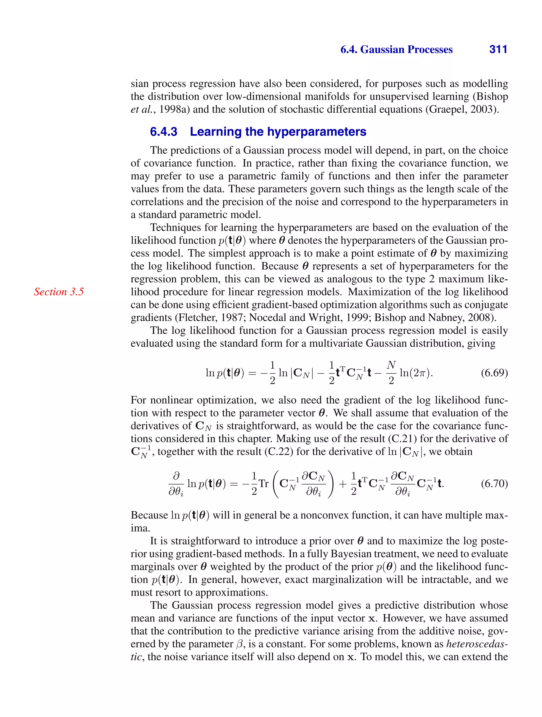
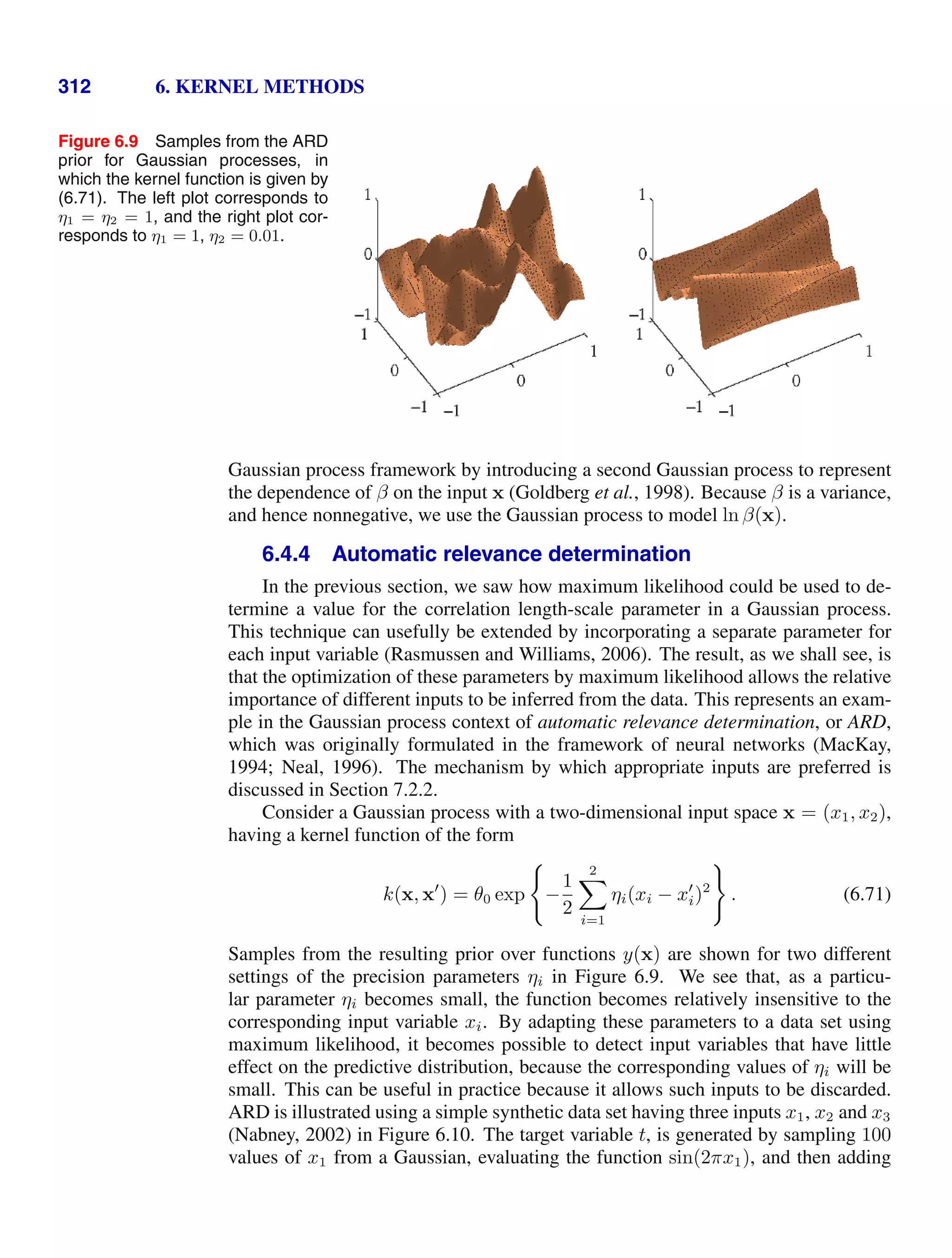
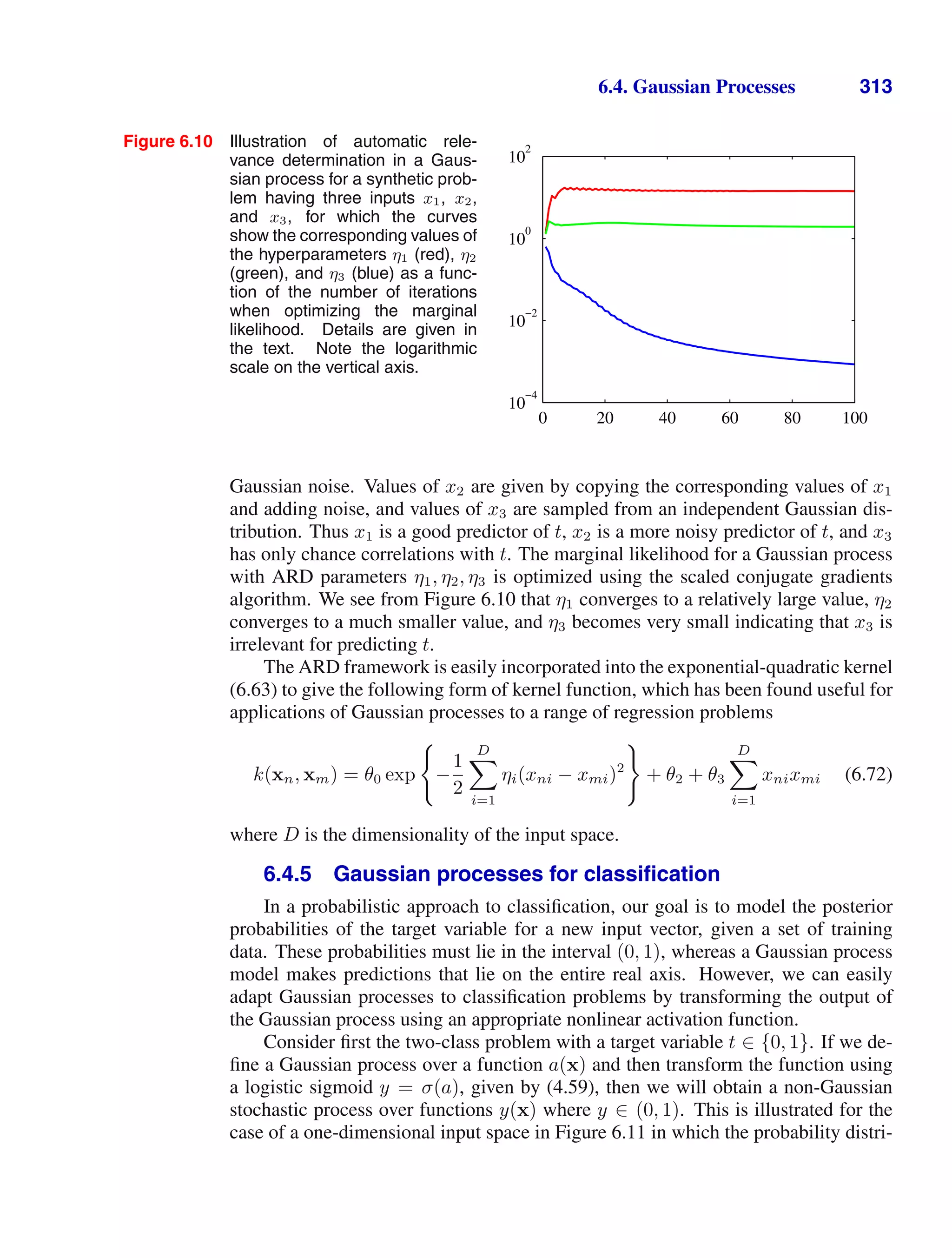
![6.4. Gaussian Processes 317
maximum. The posterior distribution is not Gaussian, however, because the Hessian
is a function of aN .
Using the Newton-Raphson formula (4.92), the iterative update equation for aN
is given by
Exercise 6.25
anew
N = CN (I + WN CN )−1
{tN − σN + WN aN } . (6.83)
These equations are iterated until they converge to the mode which we denote by
a
N . At the mode, the gradient ∇Ψ(aN ) will vanish, and hence a
N will satisfy
a
N = CN (tN − σN ). (6.84)
Once we have found the mode a
N of the posterior, we can evaluate the Hessian
matrix given by
H = −∇∇Ψ(aN ) = WN + C−1
N (6.85)
where the elements of WN are evaluated using a
N . This defines our Gaussian ap-
proximation to the posterior distribution p(aN |tN ) given by
q(aN ) = N(aN |a
N , H−1
). (6.86)
We can now combine this with (6.78) and hence evaluate the integral (6.77). Because
this corresponds to a linear-Gaussian model, we can use the general result (2.115) to
give
Exercise 6.26
E[aN+1|tN ] = kT
(tN − σN ) (6.87)
var[aN+1|tN ] = c − kT
(W−1
N + CN )−1
k. (6.88)
Now that we have a Gaussian distribution for p(aN+1|tN ), we can approximate
the integral (6.76) using the result (4.153). As with the Bayesian logistic regression
model of Section 4.5, if we are only interested in the decision boundary correspond-
ing to p(tN+1|tN ) = 0.5, then we need only consider the mean and we can ignore
the effect of the variance.
We also need to determine the parameters θ of the covariance function. One
approach is to maximize the likelihood function given by p(tN |θ) for which we need
expressions for the log likelihood and its gradient. If desired, suitable regularization
terms can also be added, leading to a penalized maximum likelihood solution. The
likelihood function is defined by
p(tN |θ) =
p(tN |aN )p(aN |θ) daN . (6.89)
This integral is analytically intractable, so again we make use of the Laplace approx-
imation. Using the result (4.135), we obtain the following approximation for the log
of the likelihood function
ln p(tN |θ) = Ψ(a
N ) −
1
2
ln |WN + C−1
N | +
N
2
ln(2π) (6.90)](https://image.slidesharecdn.com/bishop-patternrecognitionandmachinelearning-230316082240-9af1cdaa/75/Bishop-Pattern-Recognition-and-Machine-Learning-pdf-334-2048.jpg)
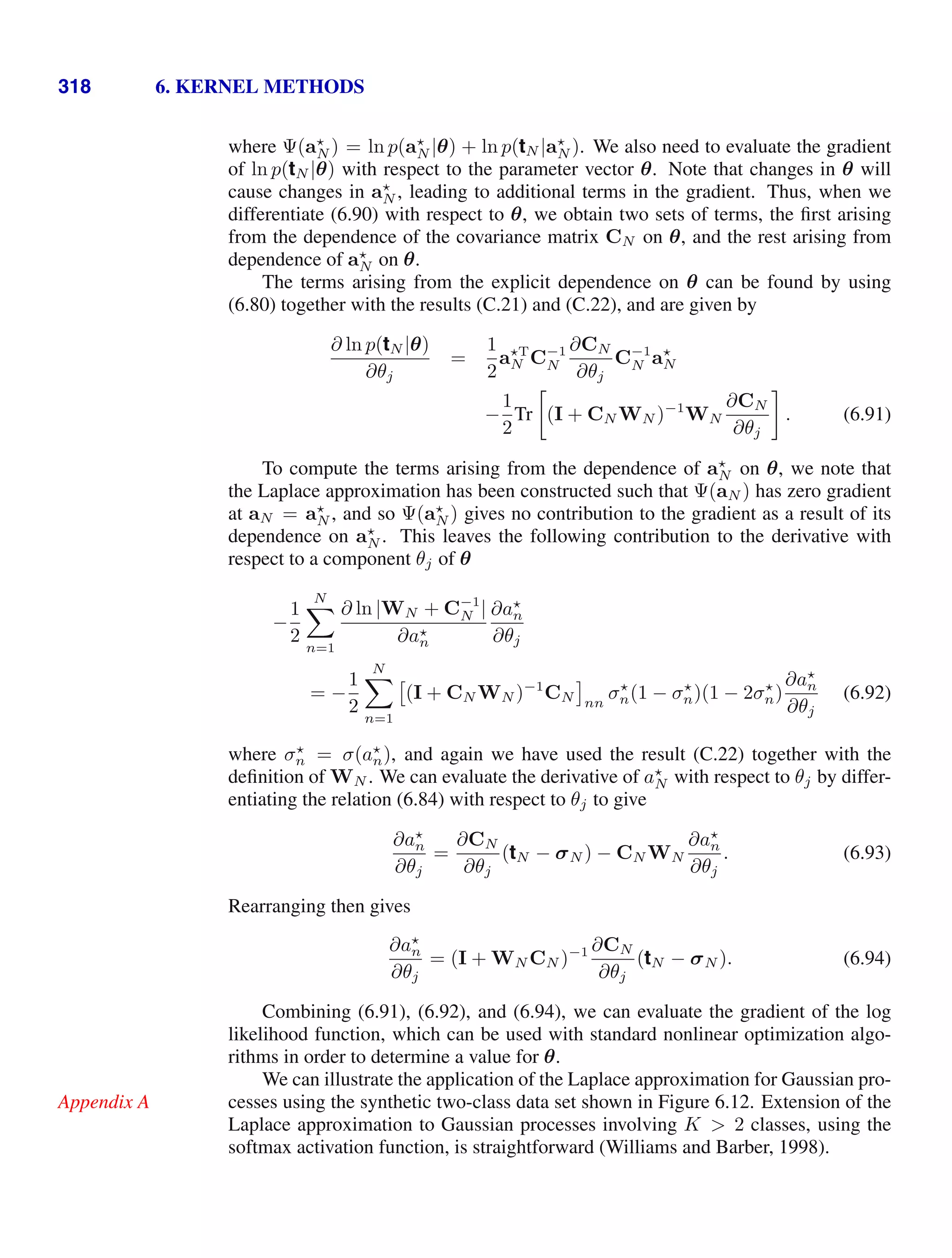
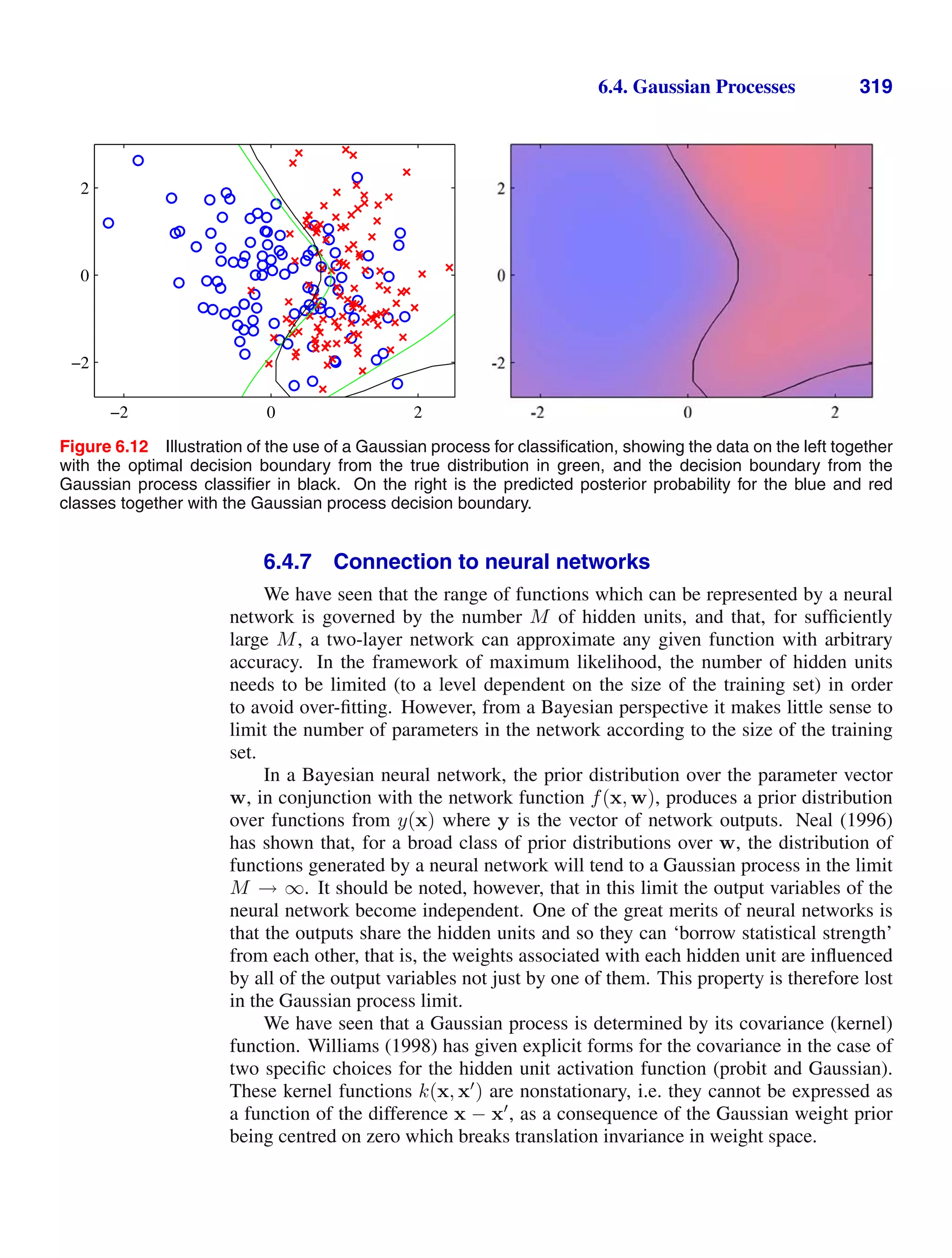
![322 6. KERNEL METHODS
6.18 ( ) Consider a Nadaraya-Watson model with one input variable x and one target
variable t having Gaussian components with isotropic covariances, so that the co-
variance matrix is given by σ2
I where I is the unit matrix. Write down expressions
for the conditional density p(t|x) and for the conditional mean E[t|x] and variance
var[t|x], in terms of the kernel function k(x, xn).
6.19 ( ) Another viewpoint on kernel regression comes from a consideration of re-
gression problems in which the input variables as well as the target variables are
corrupted with additive noise. Suppose each target value tn is generated as usual
by taking a function y(zn) evaluated at a point zn, and adding Gaussian noise. The
value of zn is not directly observed, however, but only a noise corrupted version
xn = zn + ξn where the random variable ξ is governed by some distribution g(ξ).
Consider a set of observations {xn, tn}, where n = 1, . . . , N, together with a cor-
responding sum-of-squares error function defined by averaging over the distribution
of input noise to give
E =
1
2
N
n=1
{y(xn − ξn) − tn}
2
g(ξn) dξn. (6.99)
By minimizing E with respect to the function y(z) using the calculus of variations
(Appendix D), show that optimal solution for y(x) is given by a Nadaraya-Watson
kernel regression solution of the form (6.45) with a kernel of the form (6.46).
6.20 ( ) www Verify the results (6.66) and (6.67).
6.21 ( ) www Consider a Gaussian process regression model in which the kernel
function is defined in terms of a fixed set of nonlinear basis functions. Show that the
predictive distribution is identical to the result (3.58) obtained in Section 3.3.2 for the
Bayesian linear regression model. To do this, note that both models have Gaussian
predictive distributions, and so it is only necessary to show that the conditional mean
and variance are the same. For the mean, make use of the matrix identity (C.6), and
for the variance, make use of the matrix identity (C.7).
6.22 ( ) Consider a regression problem with N training set input vectors x1, . . . , xN
and L test set input vectors xN+1, . . . , xN+L, and suppose we define a Gaussian
process prior over functions t(x). Derive an expression for the joint predictive dis-
tribution for t(xN+1), . . . , t(xN+L), given the values of t(x1), . . . , t(xN ). Show the
marginal of this distribution for one of the test observations tj where N + 1 j
N + L is given by the usual Gaussian process regression result (6.66) and (6.67).
6.23 ( ) www Consider a Gaussian process regression model in which the target
variable t has dimensionality D. Write down the conditional distribution of tN+1
for a test input vector xN+1, given a training set of input vectors x1, . . . , xN+1 and
corresponding target observations t1, . . . , tN .
6.24 ( ) Show that a diagonal matrix W whose elements satisfy 0 Wii 1 is positive
definite. Show that the sum of two positive definite matrices is itself positive definite.](https://image.slidesharecdn.com/bishop-patternrecognitionandmachinelearning-230316082240-9af1cdaa/75/Bishop-Pattern-Recognition-and-Machine-Learning-pdf-339-2048.jpg)

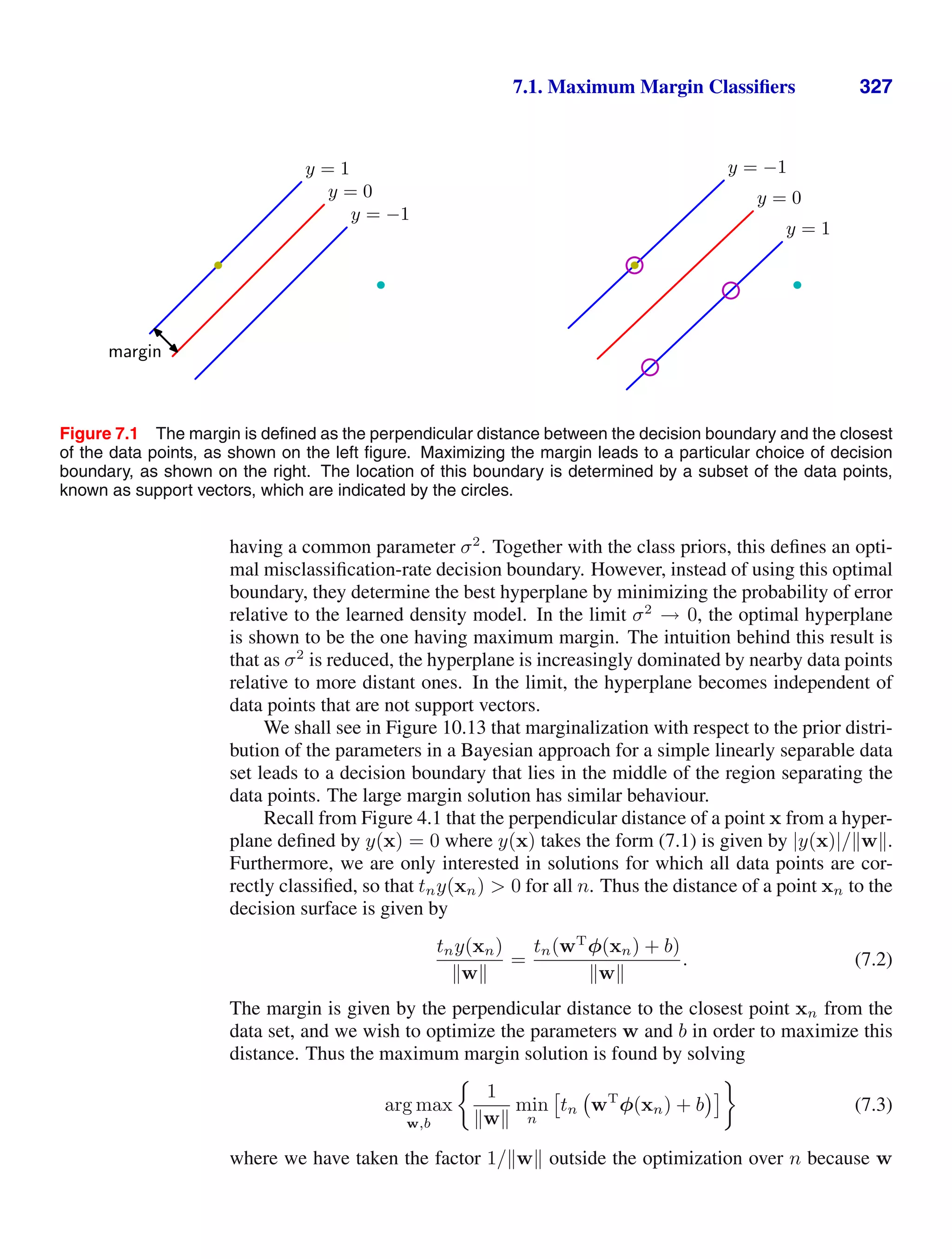
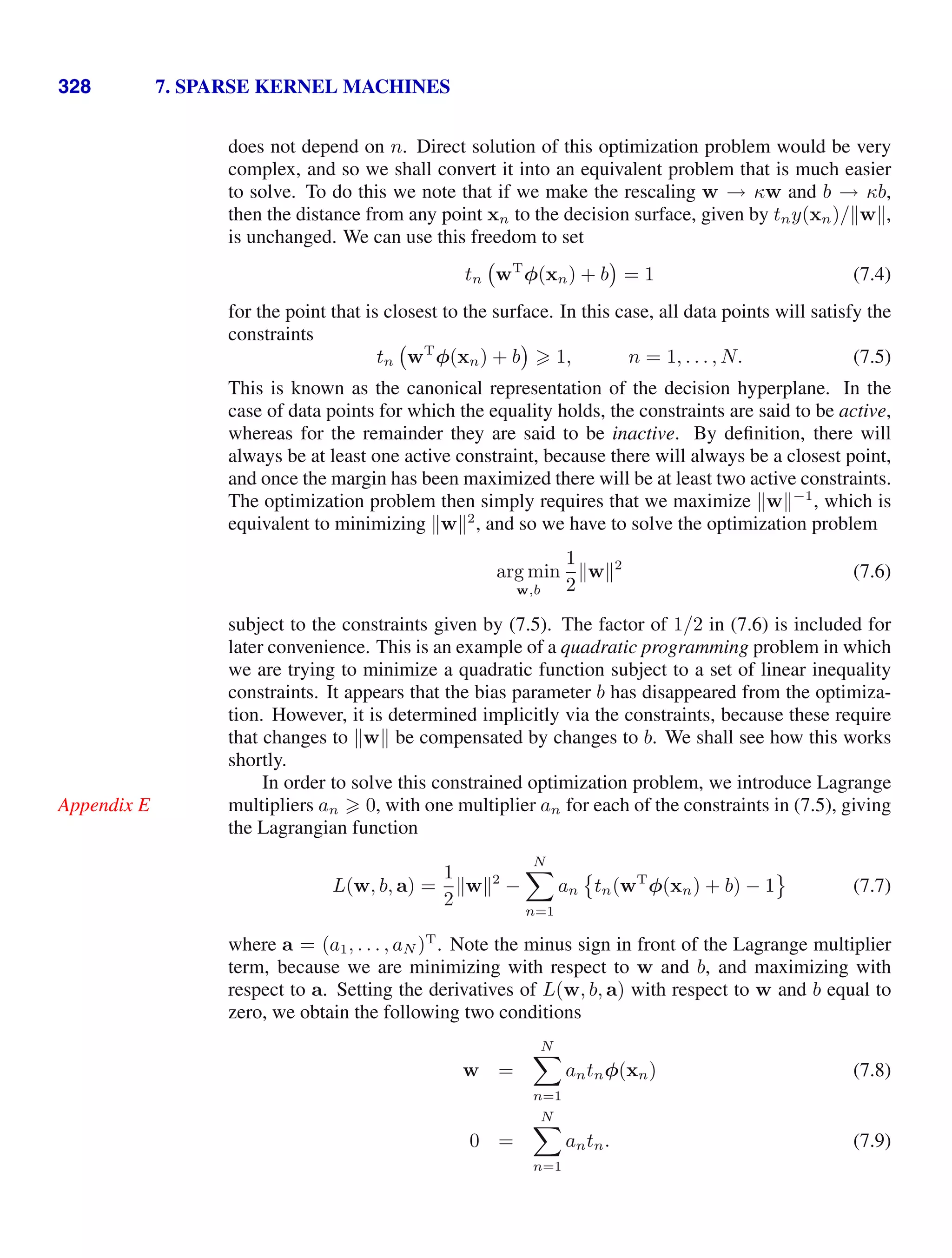
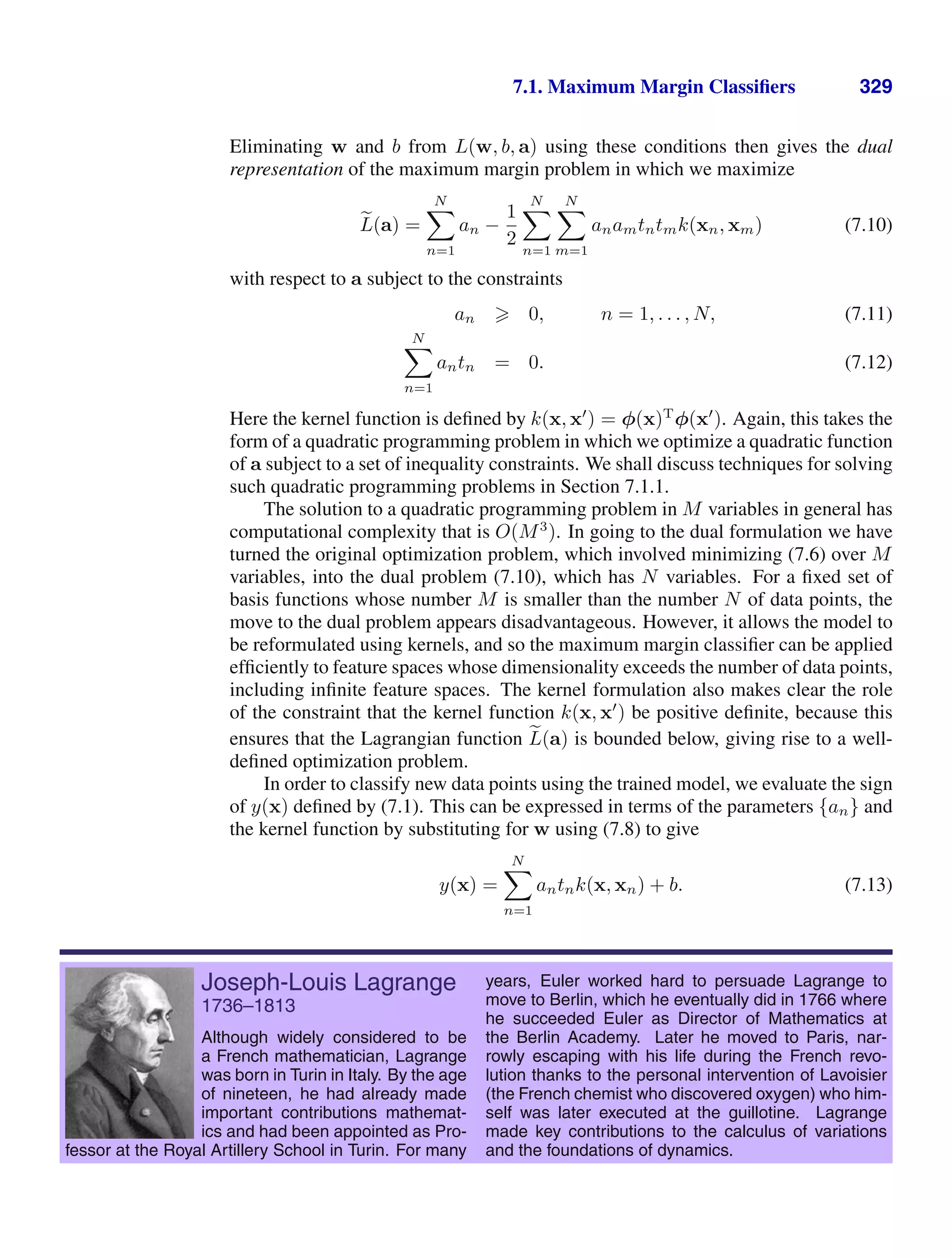
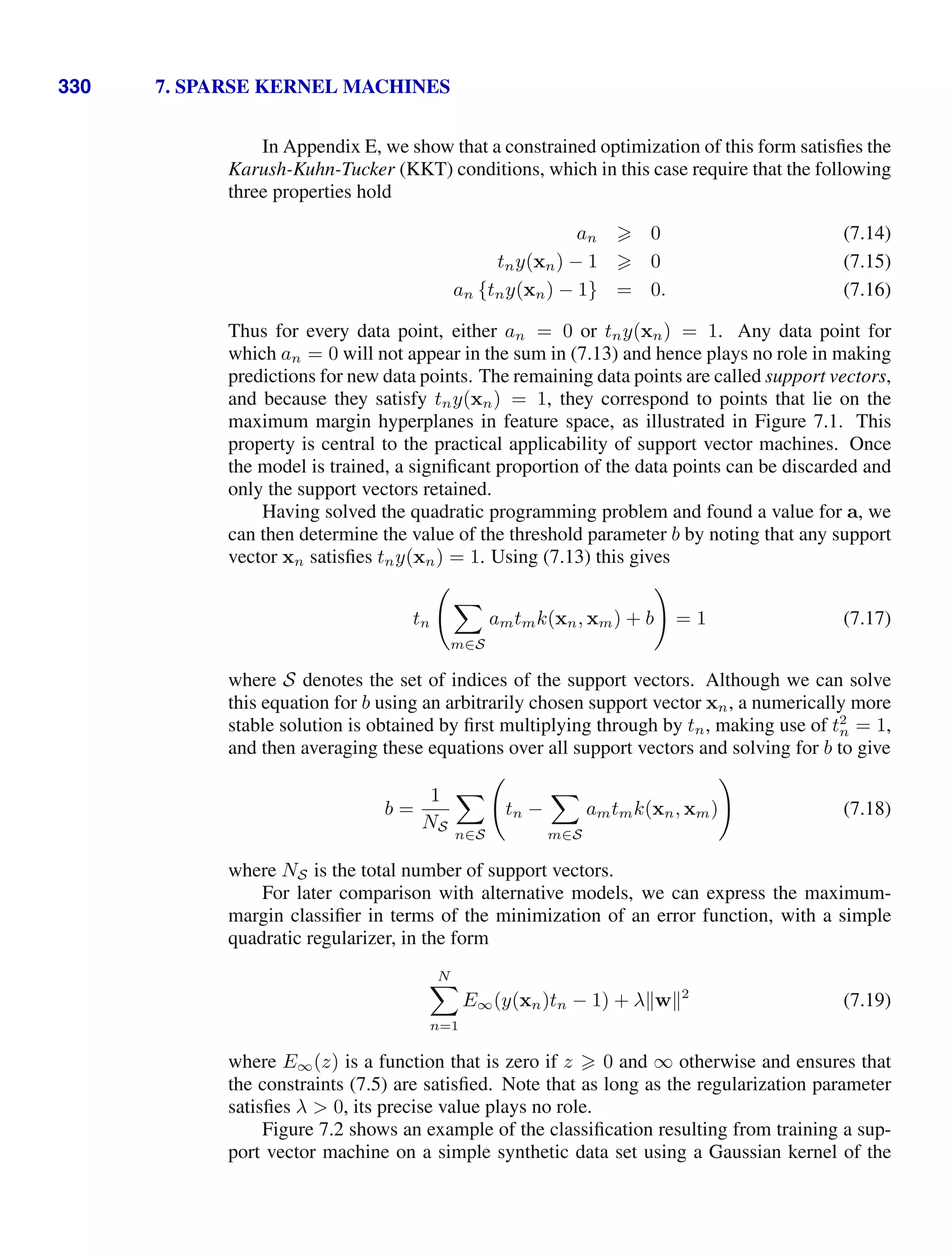
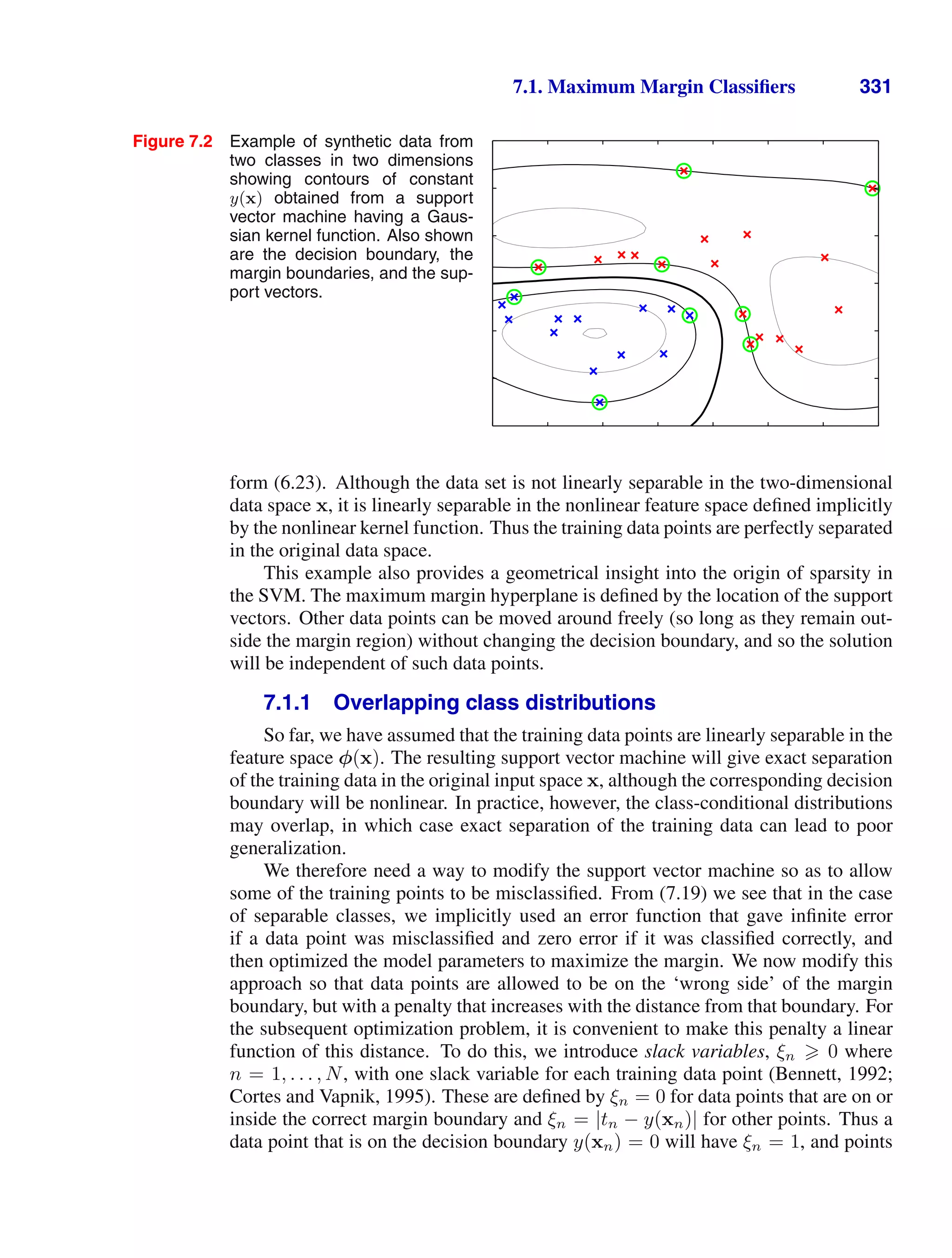
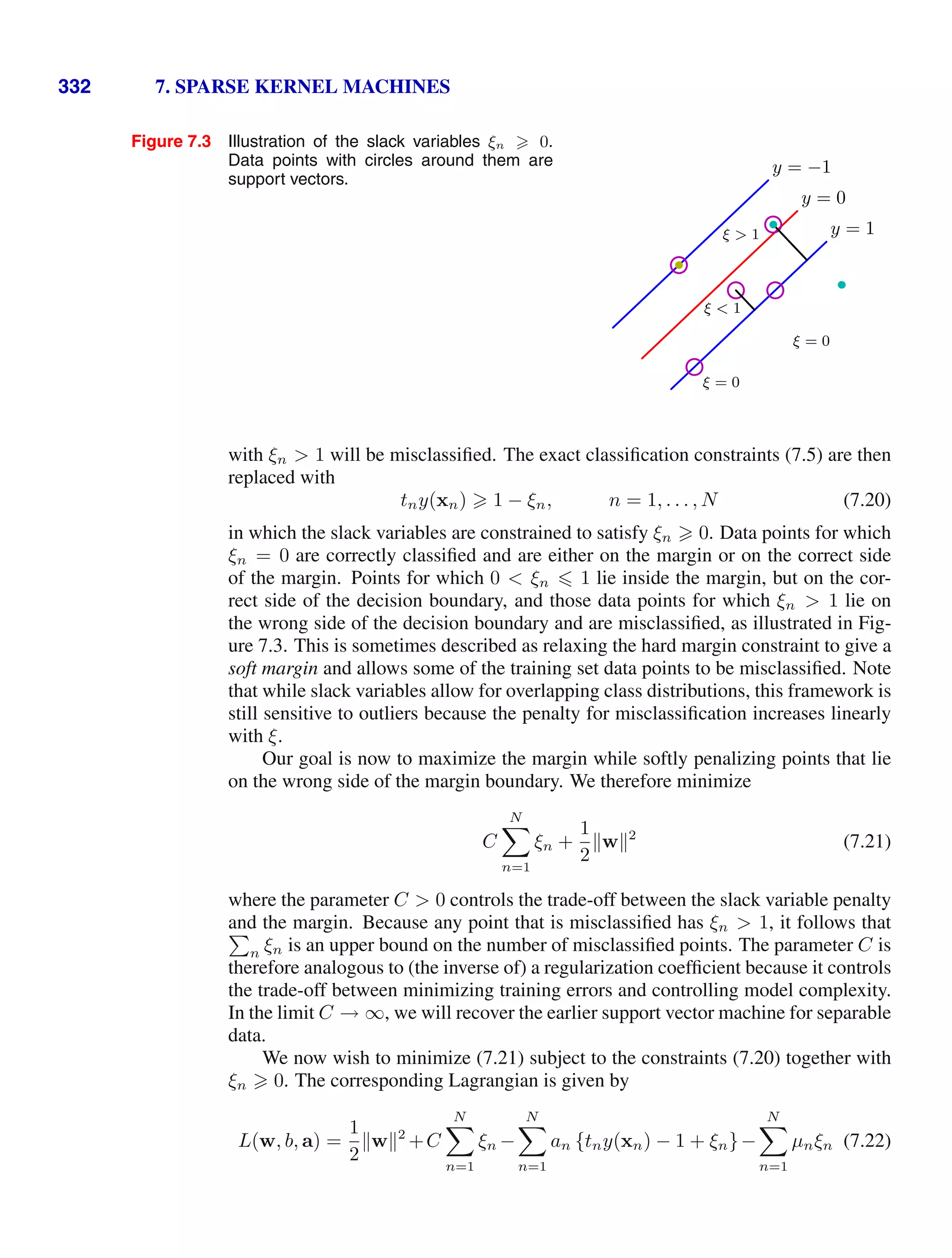
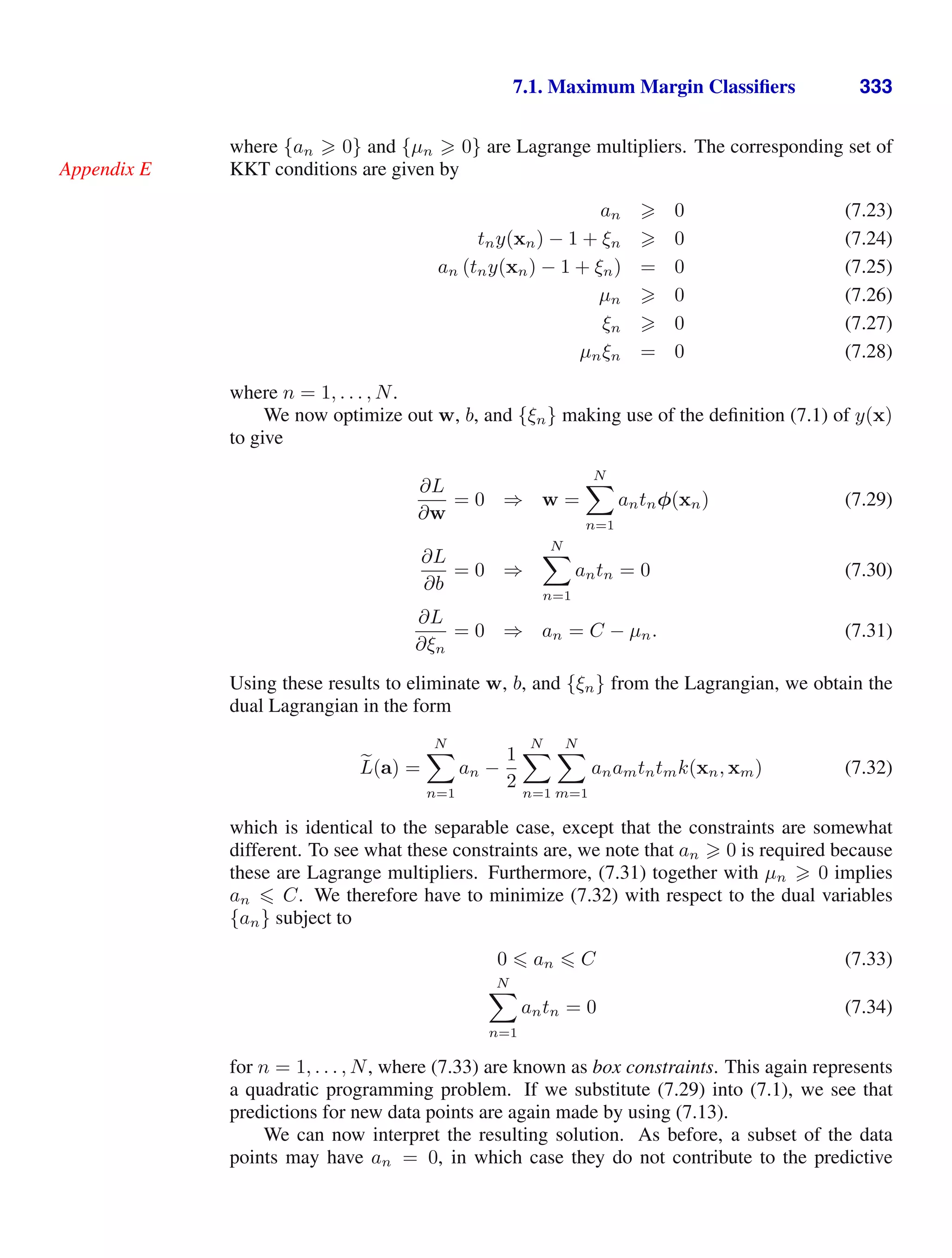
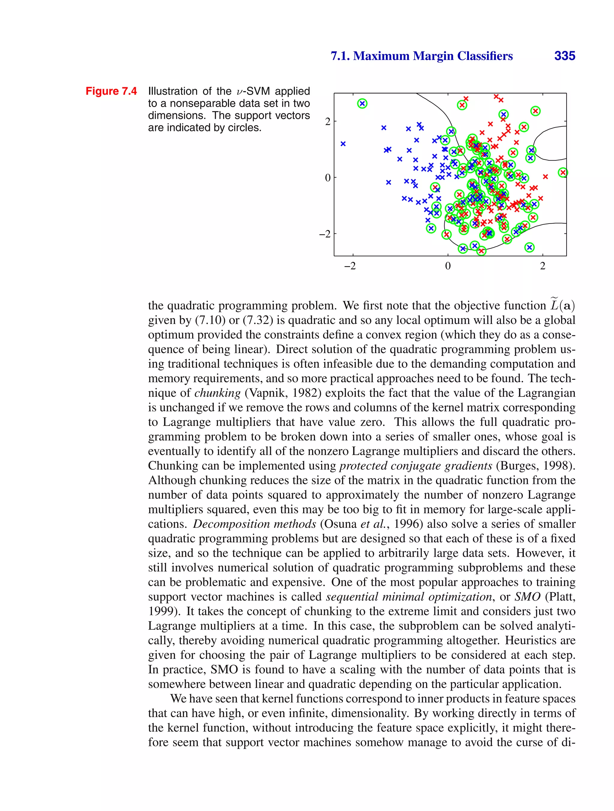
![7.1. Maximum Margin Classifiers 337
Figure 7.5 Plot of the ‘hinge’ error function used
in support vector machines, shown
in blue, along with the error function
for logistic regression, rescaled by a
factor of 1/ ln(2) so that it passes
through the point (0, 1), shown in red.
Also shown are the misclassification
error in black and the squared error
in green.
−2 −1 0 1 2
z
E(z)
remaining points we have ξn = 1 − yntn. Thus the objective function (7.21) can be
written (up to an overall multiplicative constant) in the form
N
n=1
ESV(yntn) + λw2
(7.44)
where λ = (2C)−1
, and ESV(·) is the hinge error function defined by
ESV(yntn) = [1 − yntn]+ (7.45)
where [ · ]+ denotes the positive part. The hinge error function, so-called because
of its shape, is plotted in Figure 7.5. It can be viewed as an approximation to the
misclassification error, i.e., the error function that ideally we would like to minimize,
which is also shown in Figure 7.5.
When we considered the logistic regression model in Section 4.3.2, we found it
convenient to work with target variable t ∈ {0, 1}. For comparison with the support
vector machine, we first reformulate maximum likelihood logistic regression using
the target variable t ∈ {−1, 1}. To do this, we note that p(t = 1|y) = σ(y) where
y(x) is given by (7.1), and σ(y) is the logistic sigmoid function defined by (4.59). It
follows that p(t = −1|y) = 1 − σ(y) = σ(−y), where we have used the properties
of the logistic sigmoid function, and so we can write
p(t|y) = σ(yt). (7.46)
From this we can construct an error function by taking the negative logarithm of the
likelihood function that, with a quadratic regularizer, takes the form
Exercise 7.6
N
n=1
ELR(yntn) + λw2
. (7.47)
where
ELR(yt) = ln (1 + exp(−yt)) . (7.48)](https://image.slidesharecdn.com/bishop-patternrecognitionandmachinelearning-230316082240-9af1cdaa/75/Bishop-Pattern-Recognition-and-Machine-Learning-pdf-353-2048.jpg)
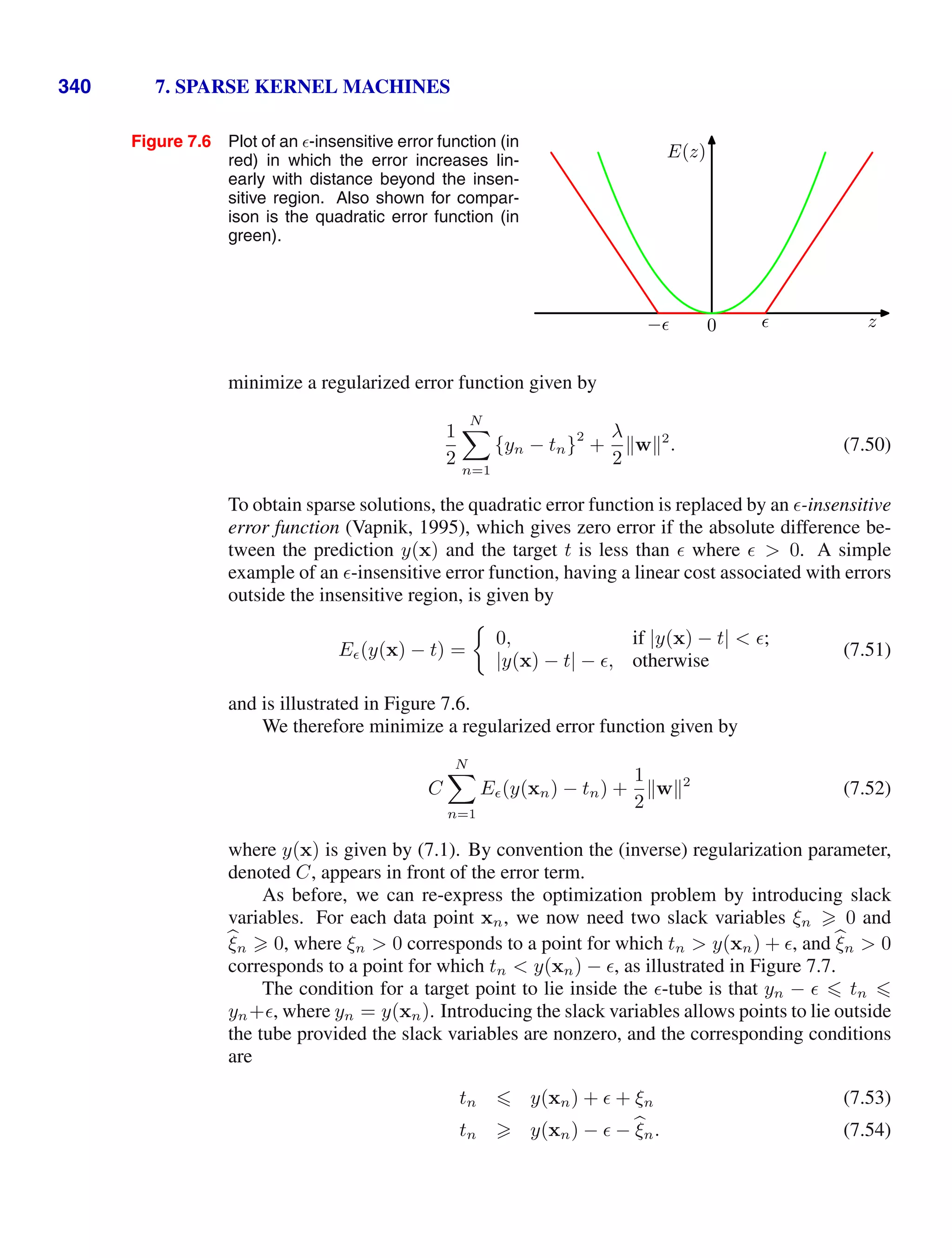
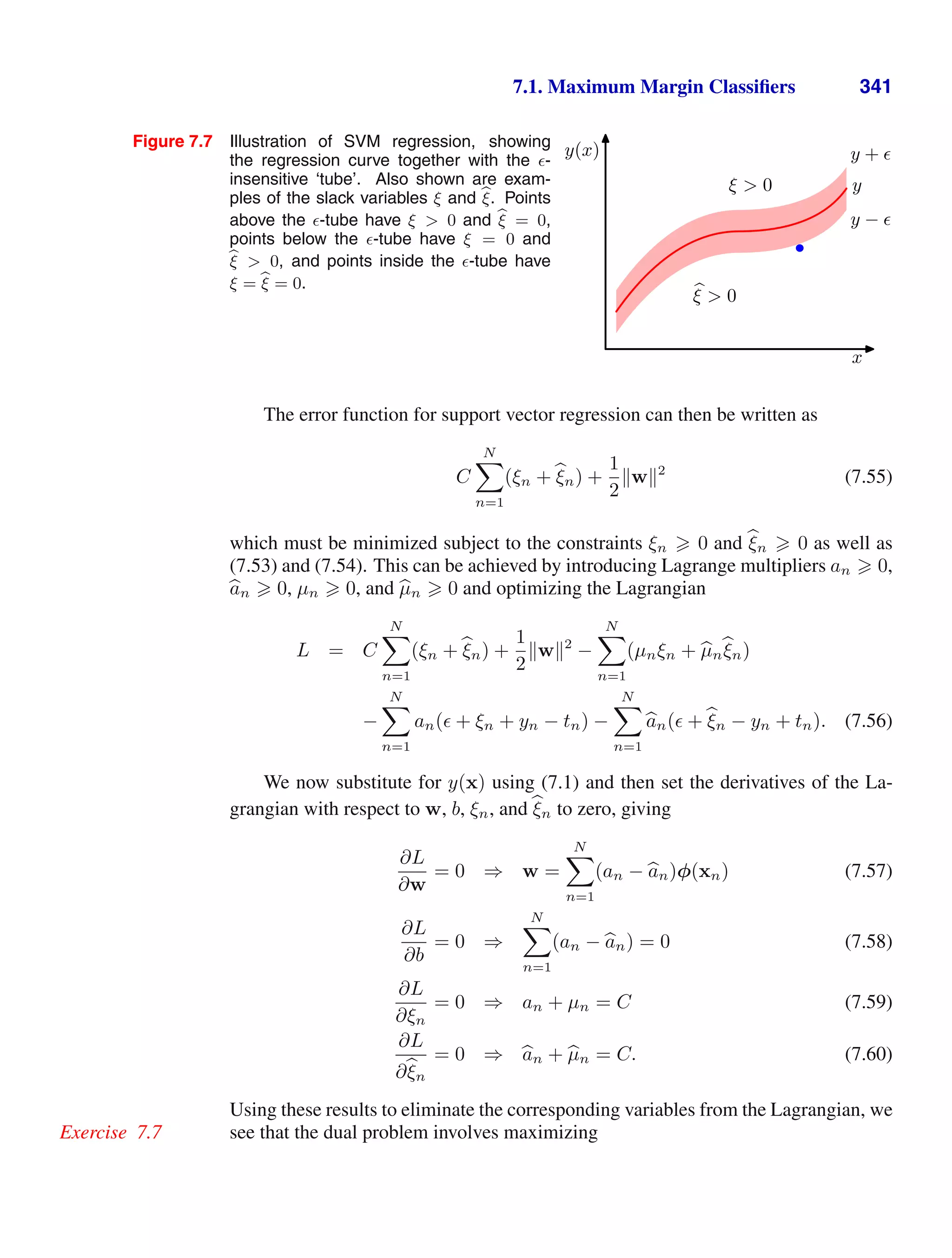
![344 7. SPARSE KERNEL MACHINES
Figure 7.8 Illustration of the ν-SVM for re-
gression applied to the sinusoidal
synthetic data set using Gaussian
kernels. The predicted regression
curve is shown by the red line, and
the -insensitive tube corresponds
to the shaded region. Also, the
data points are shown in green,
and those with support vectors
are indicated by blue circles.
x
t
0 1
−1
0
1
7.1.5 Computational learning theory
Historically, support vector machines have largely been motivated and analysed
using a theoretical framework known as computational learning theory, also some-
times called statistical learning theory (Anthony and Biggs, 1992; Kearns and Vazi-
rani, 1994; Vapnik, 1995; Vapnik, 1998). This has its origins with Valiant (1984)
who formulated the probably approximately correct, or PAC, learning framework.
The goal of the PAC framework is to understand how large a data set needs to be in
order to give good generalization. It also gives bounds for the computational cost of
learning, although we do not consider these here.
Suppose that a data set D of size N is drawn from some joint distribution p(x, t)
where x is the input variable and t represents the class label, and that we restrict
attention to ‘noise free’ situations in which the class labels are determined by some
(unknown) deterministic function t = g(x). In PAC learning we say that a function
f(x; D), drawn from a space F of such functions on the basis of the training set
D, has good generalization if its expected error rate is below some pre-specified
threshold , so that
Ex,t [I (f(x; D) = t)] (7.75)
where I(·) is the indicator function, and the expectation is with respect to the dis-
tribution p(x, t). The quantity on the left-hand side is a random variable, because
it depends on the training set D, and the PAC framework requires that (7.75) holds,
with probability greater than 1 − δ, for a data set D drawn randomly from p(x, t).
Here δ is another pre-specified parameter, and the terminology ‘probably approxi-
mately correct’ comes from the requirement that with high probability (greater than
1−δ), the error rate be small (less than ). For a given choice of model space F, and
for given parameters and δ, PAC learning aims to provide bounds on the minimum
size N of data set needed to meet this criterion. A key quantity in PAC learning is
the Vapnik-Chervonenkis dimension, or VC dimension, which provides a measure of
the complexity of a space of functions, and which allows the PAC framework to be
extended to spaces containing an infinite number of functions.
The bounds derived within the PAC framework are often described as worst-](https://image.slidesharecdn.com/bishop-patternrecognitionandmachinelearning-230316082240-9af1cdaa/75/Bishop-Pattern-Recognition-and-Machine-Learning-pdf-360-2048.jpg)
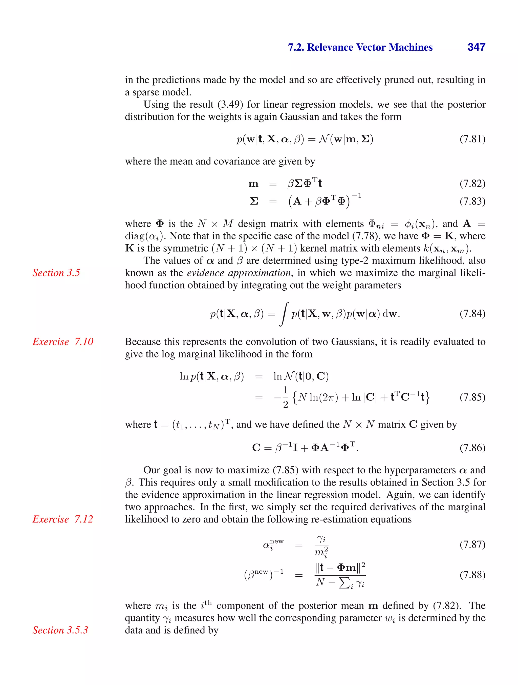
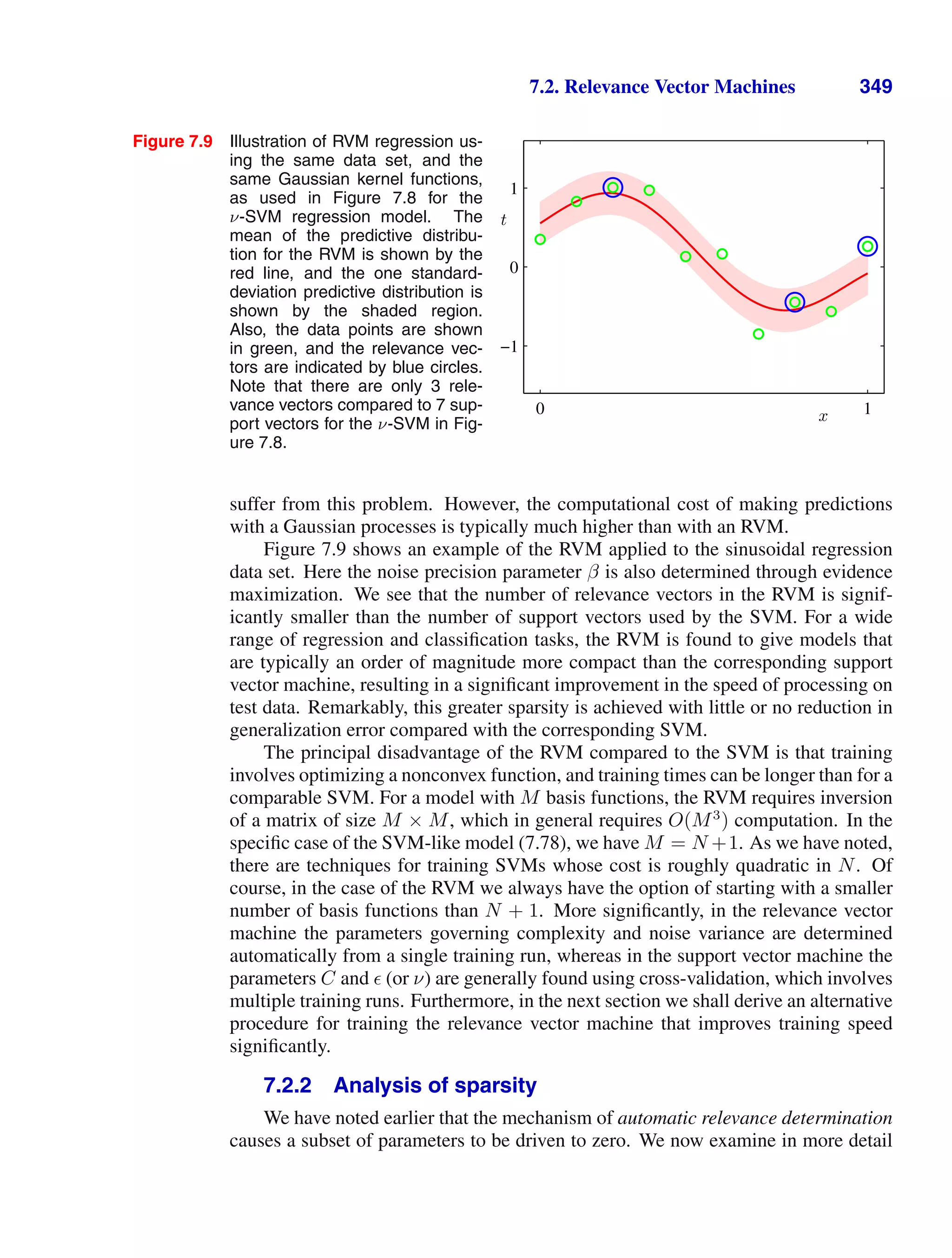
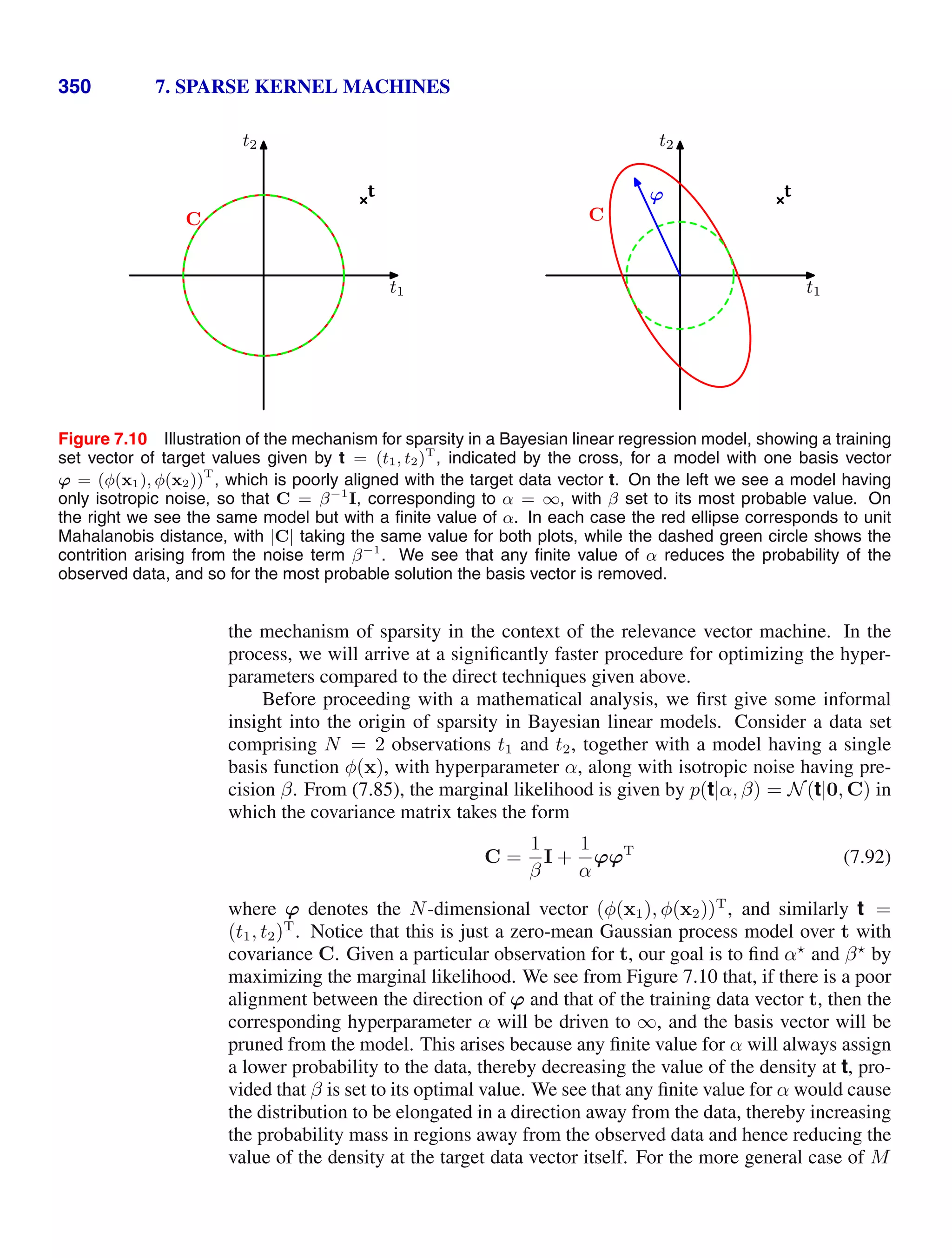
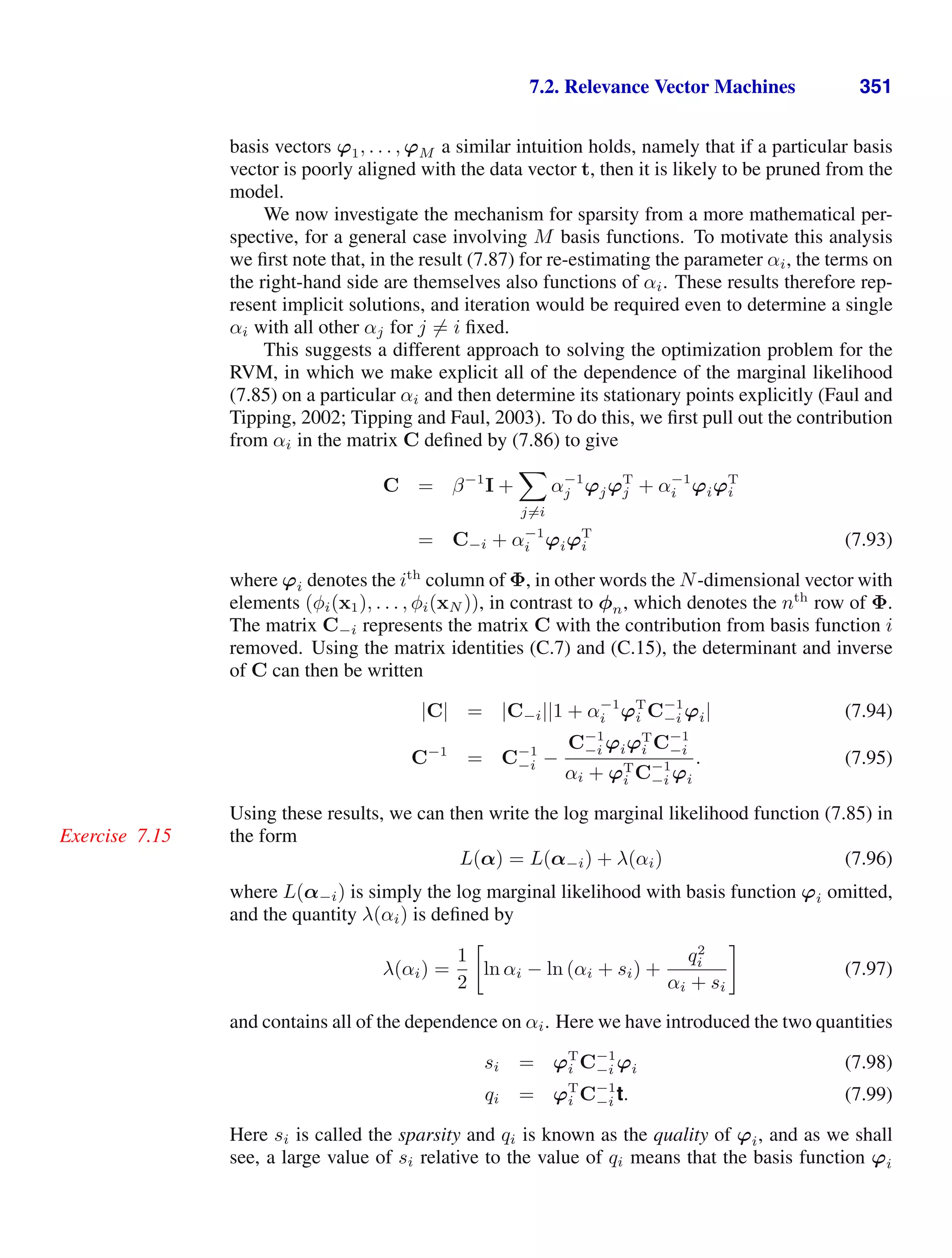
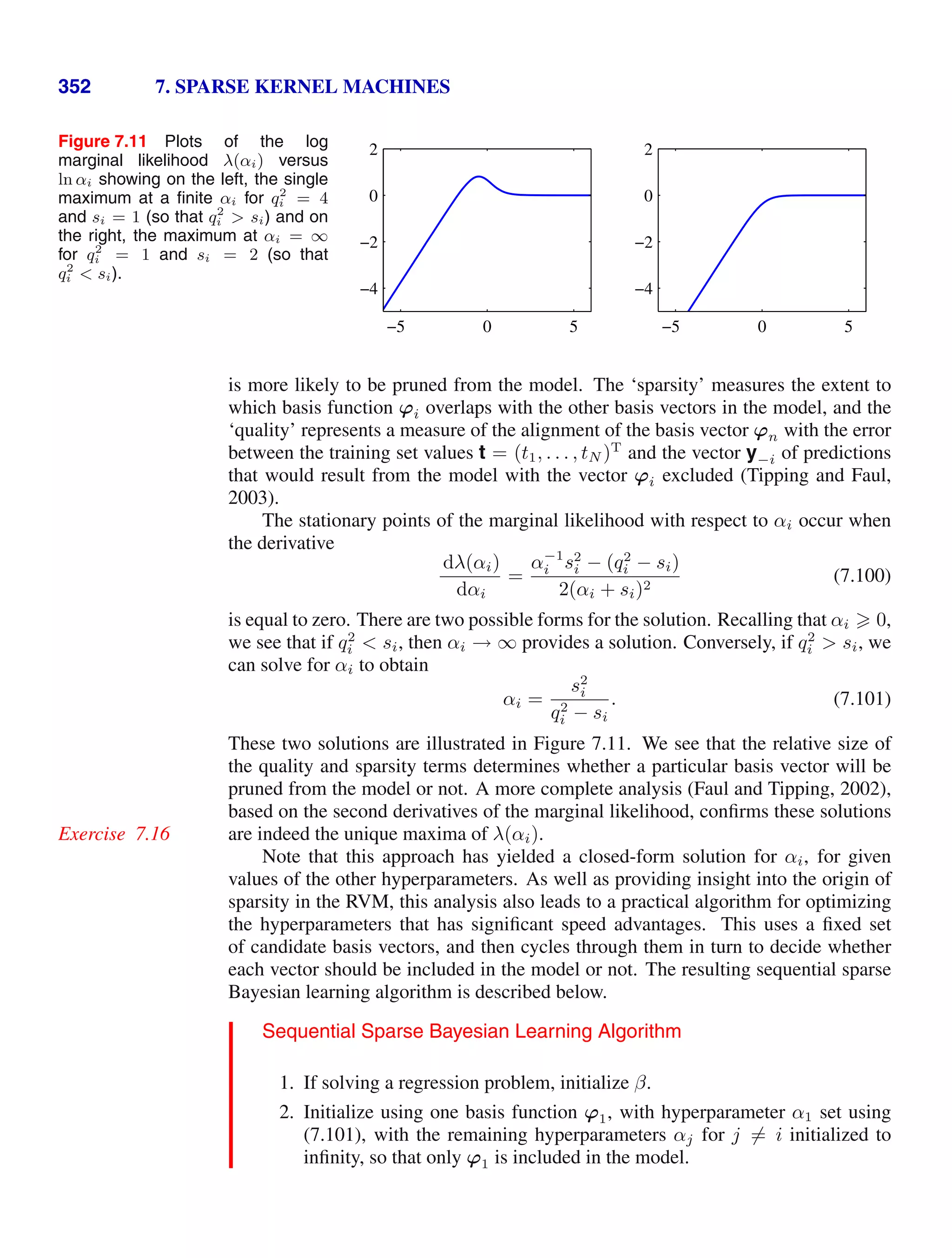
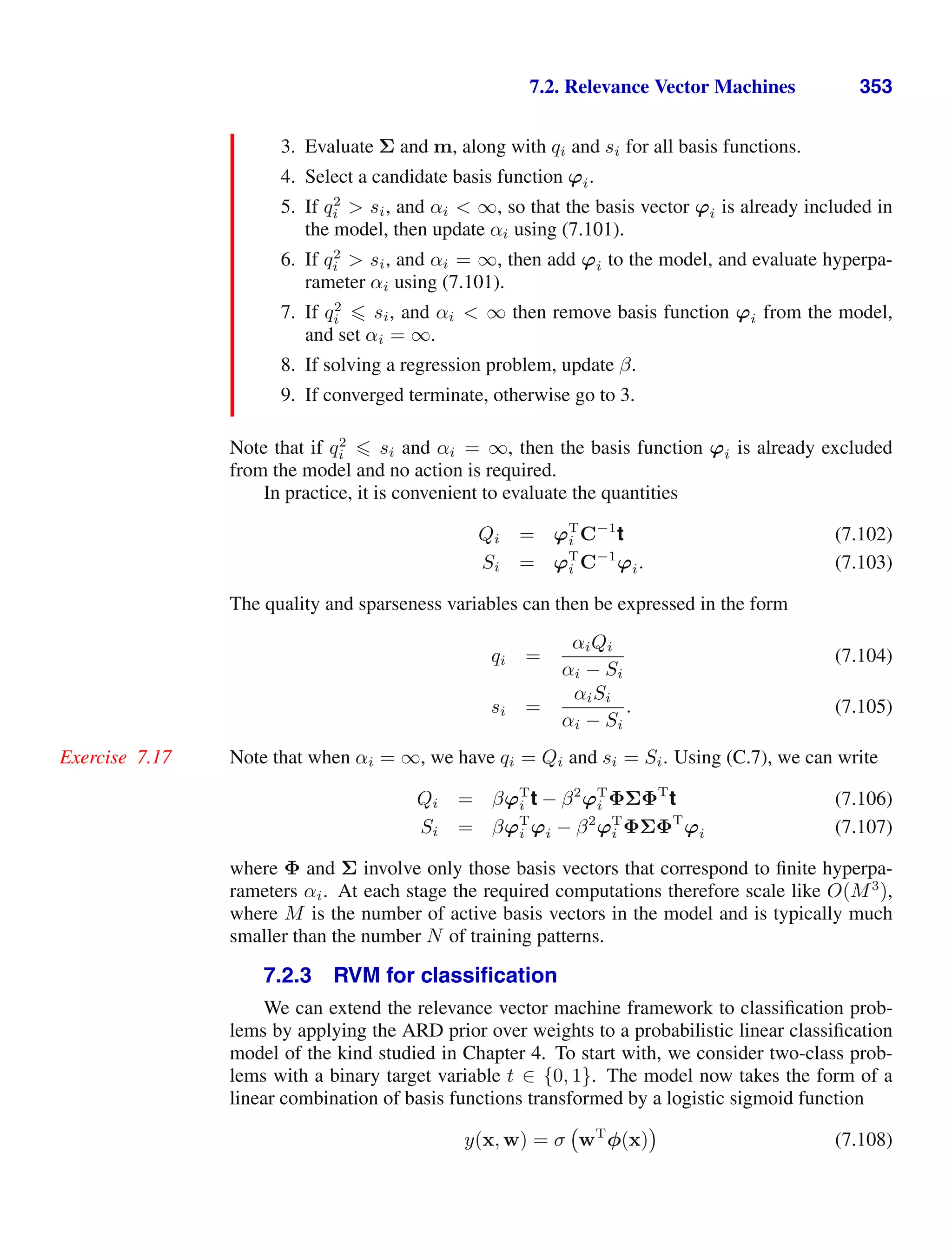
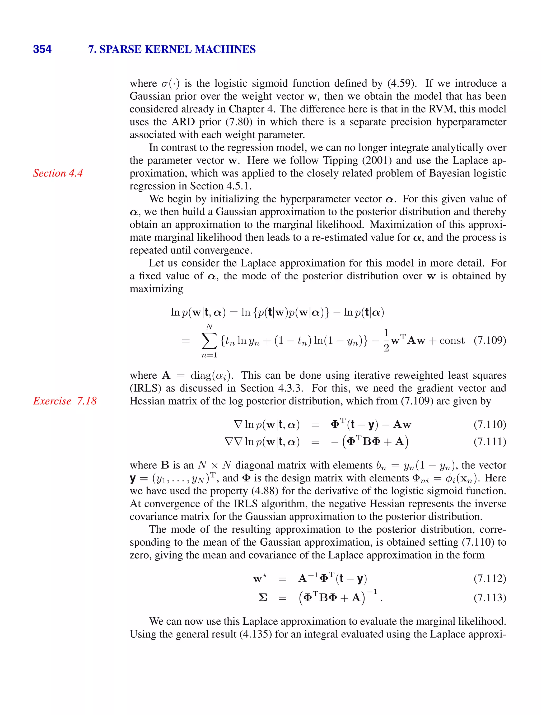
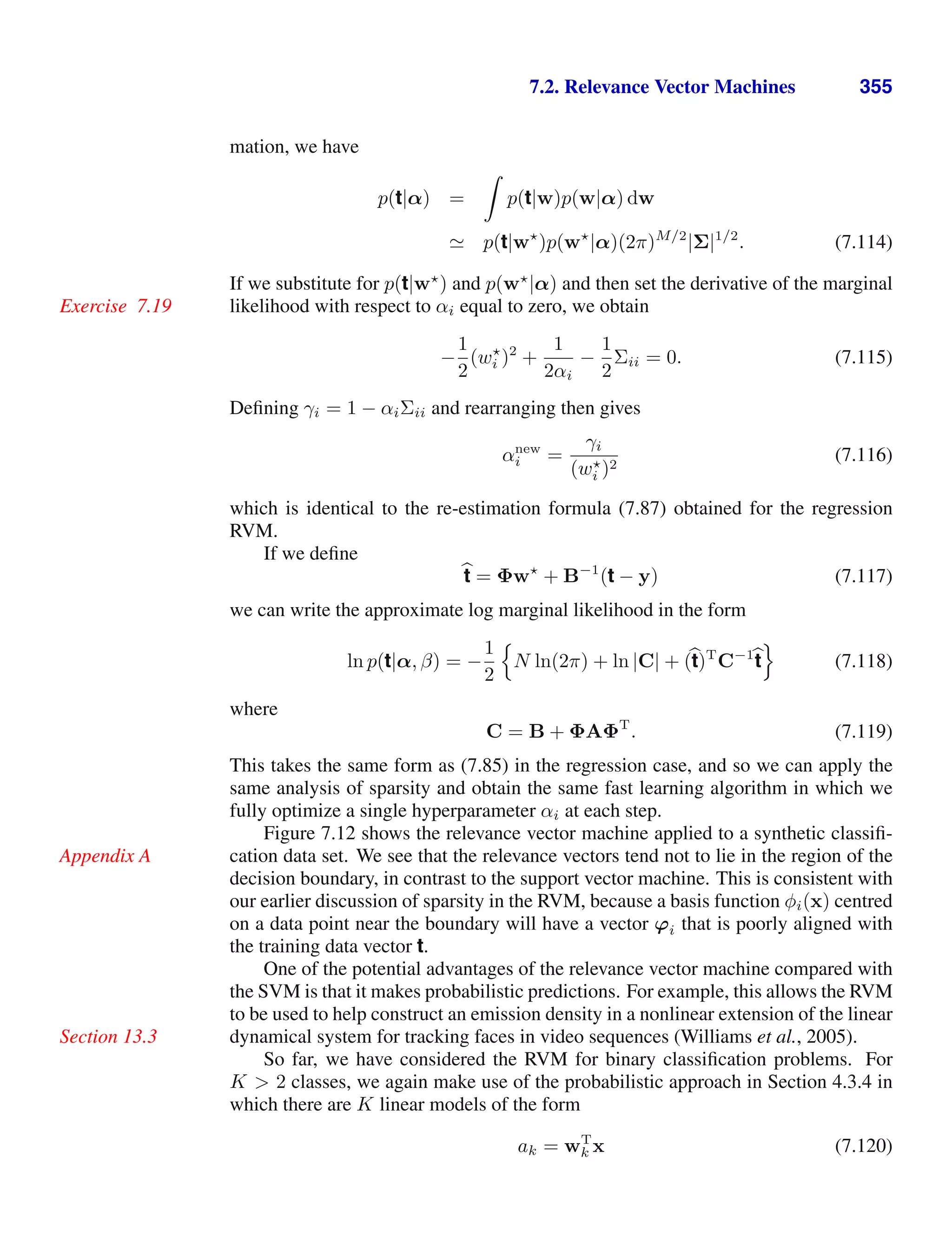

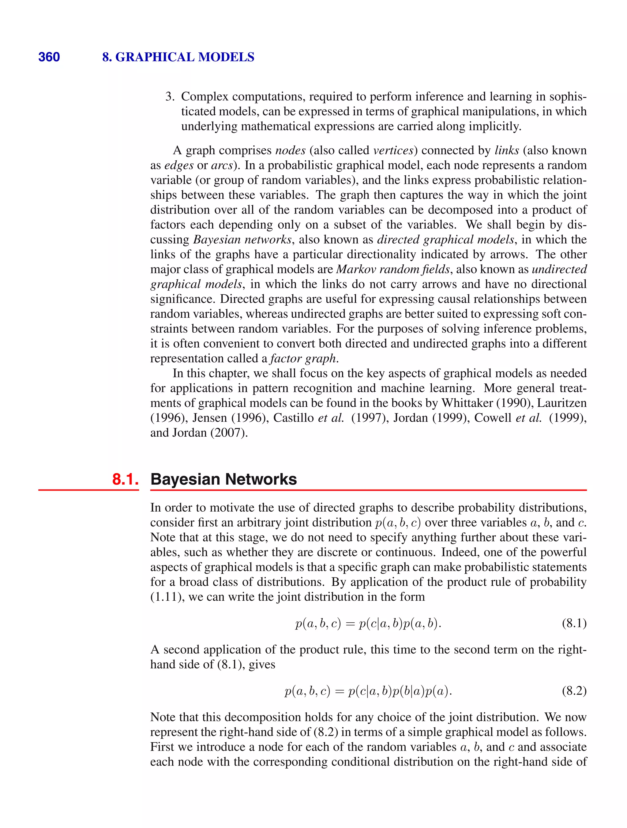
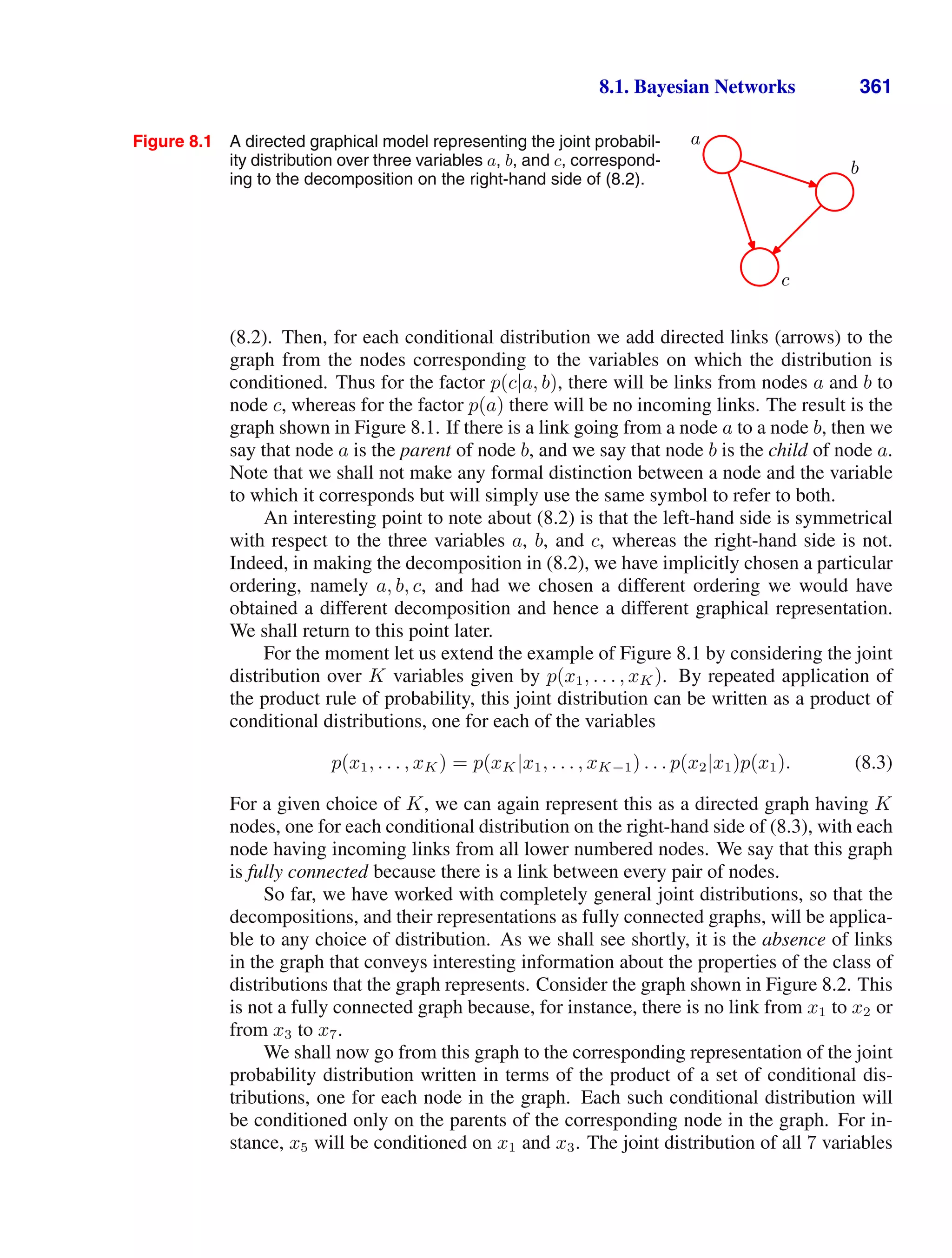
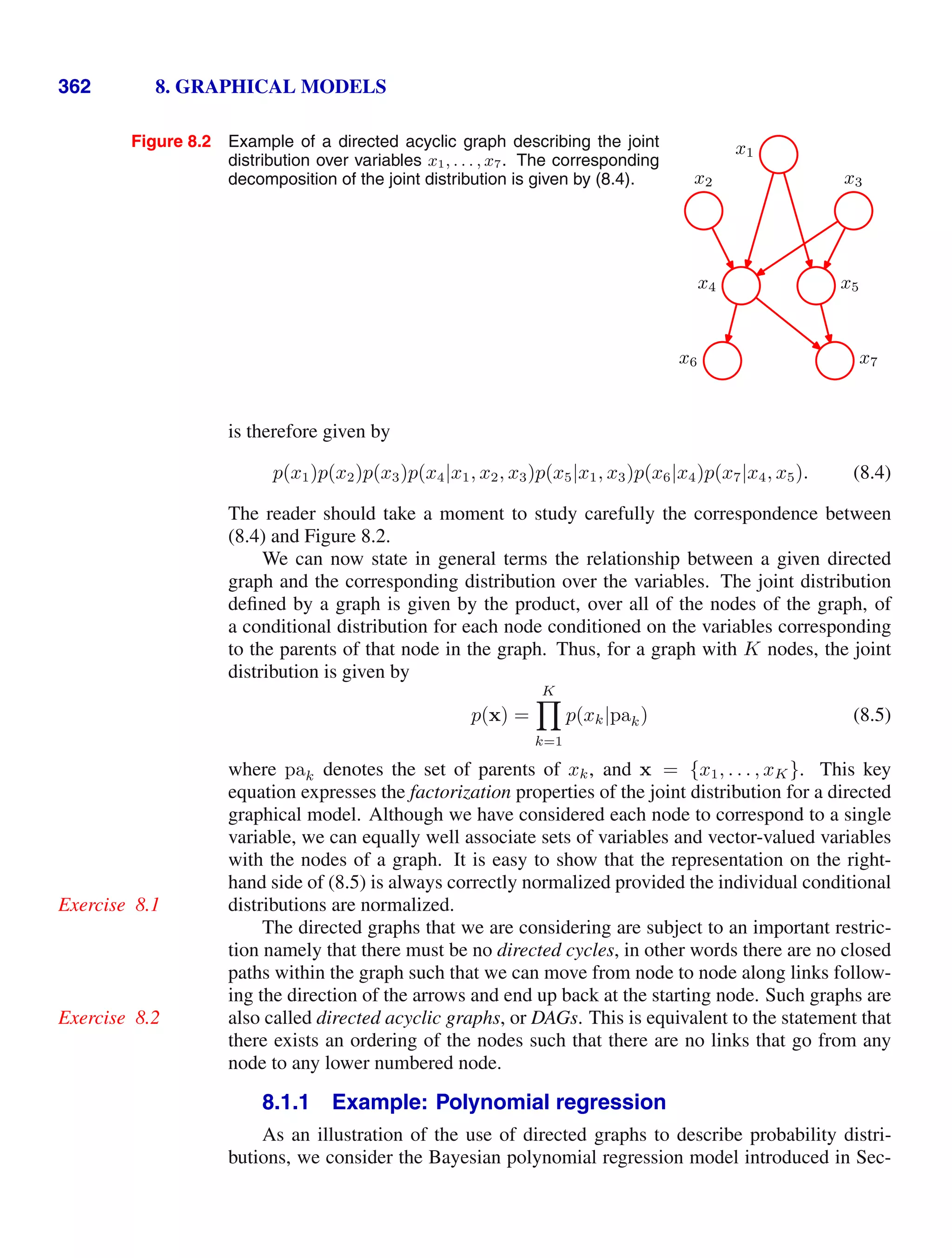
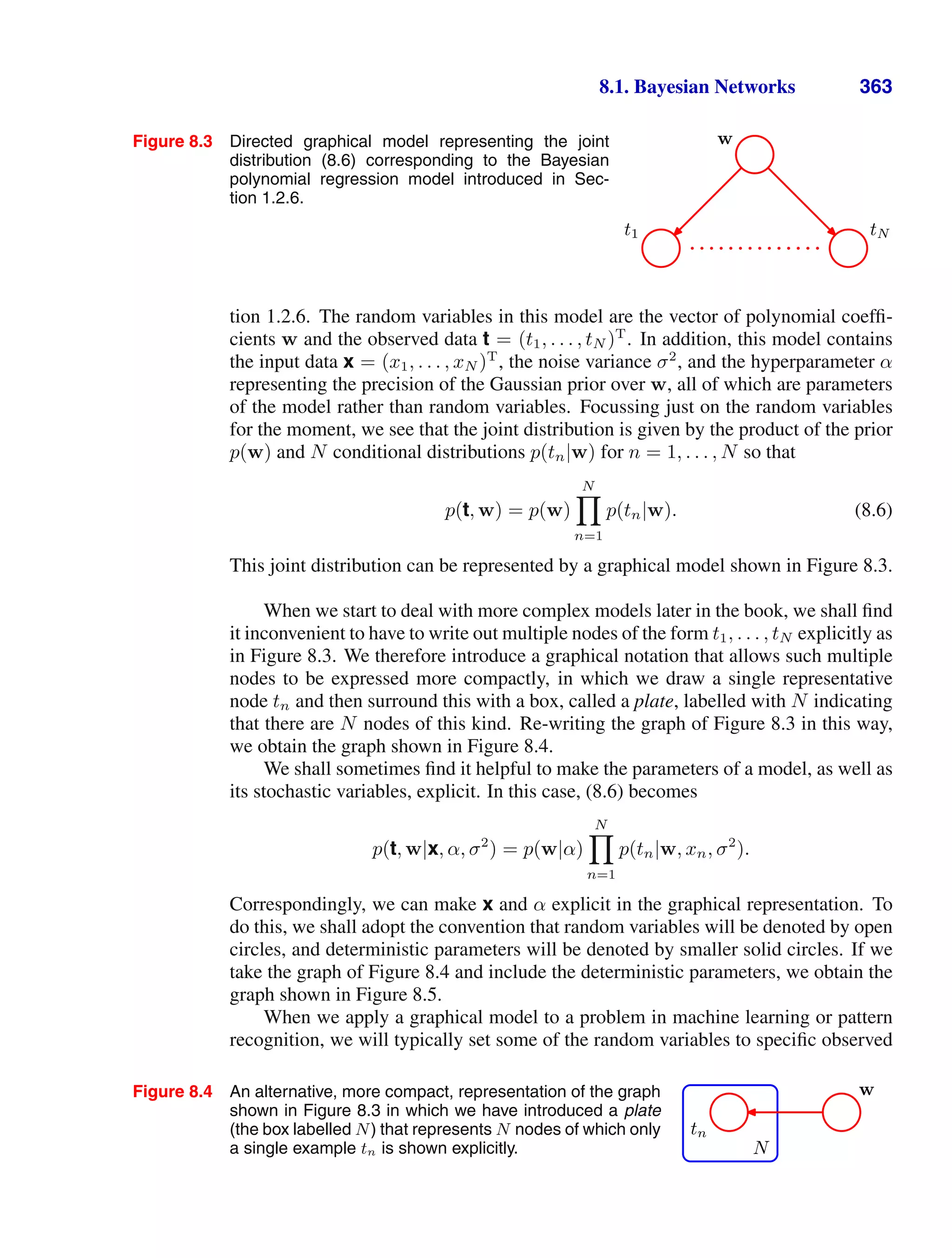
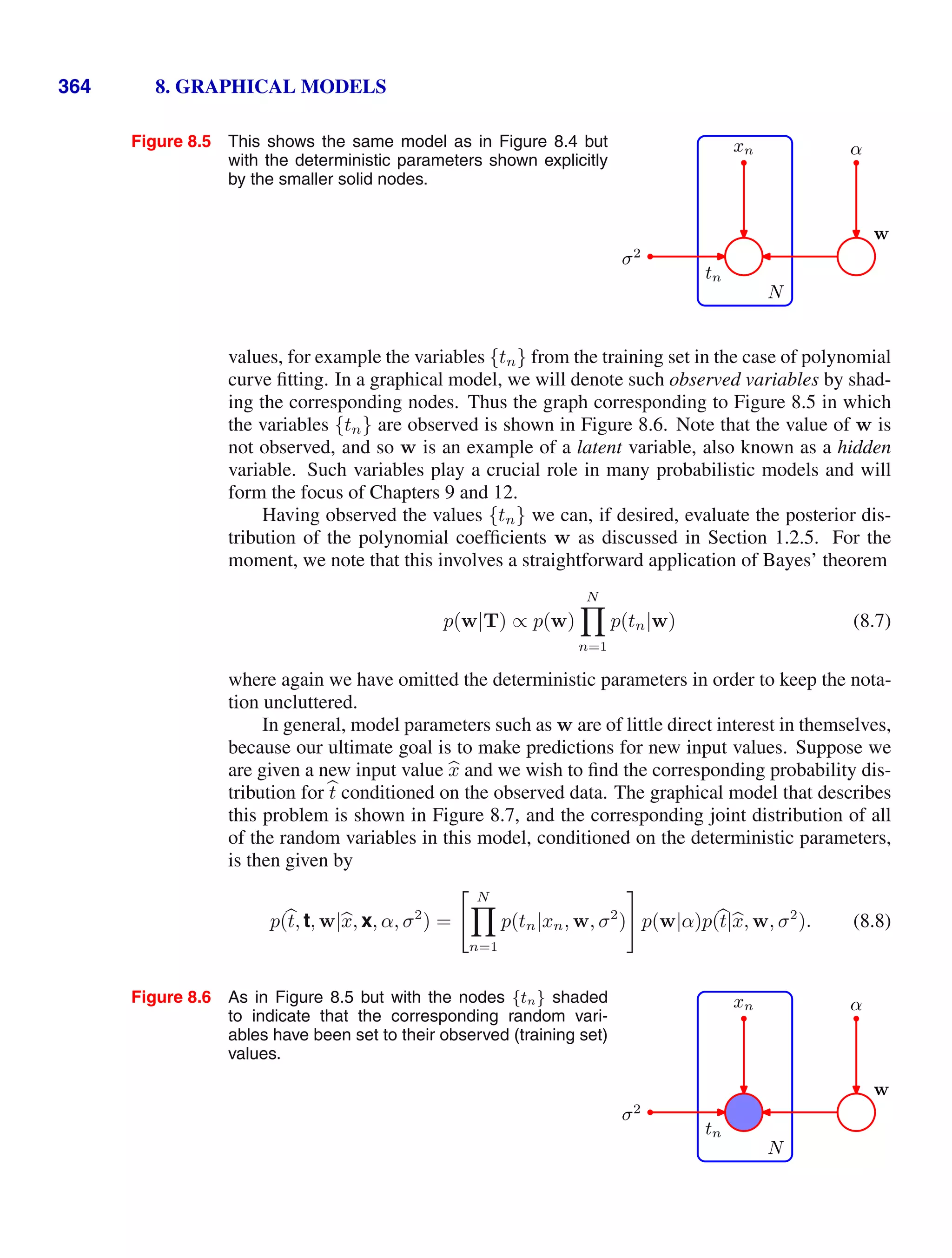
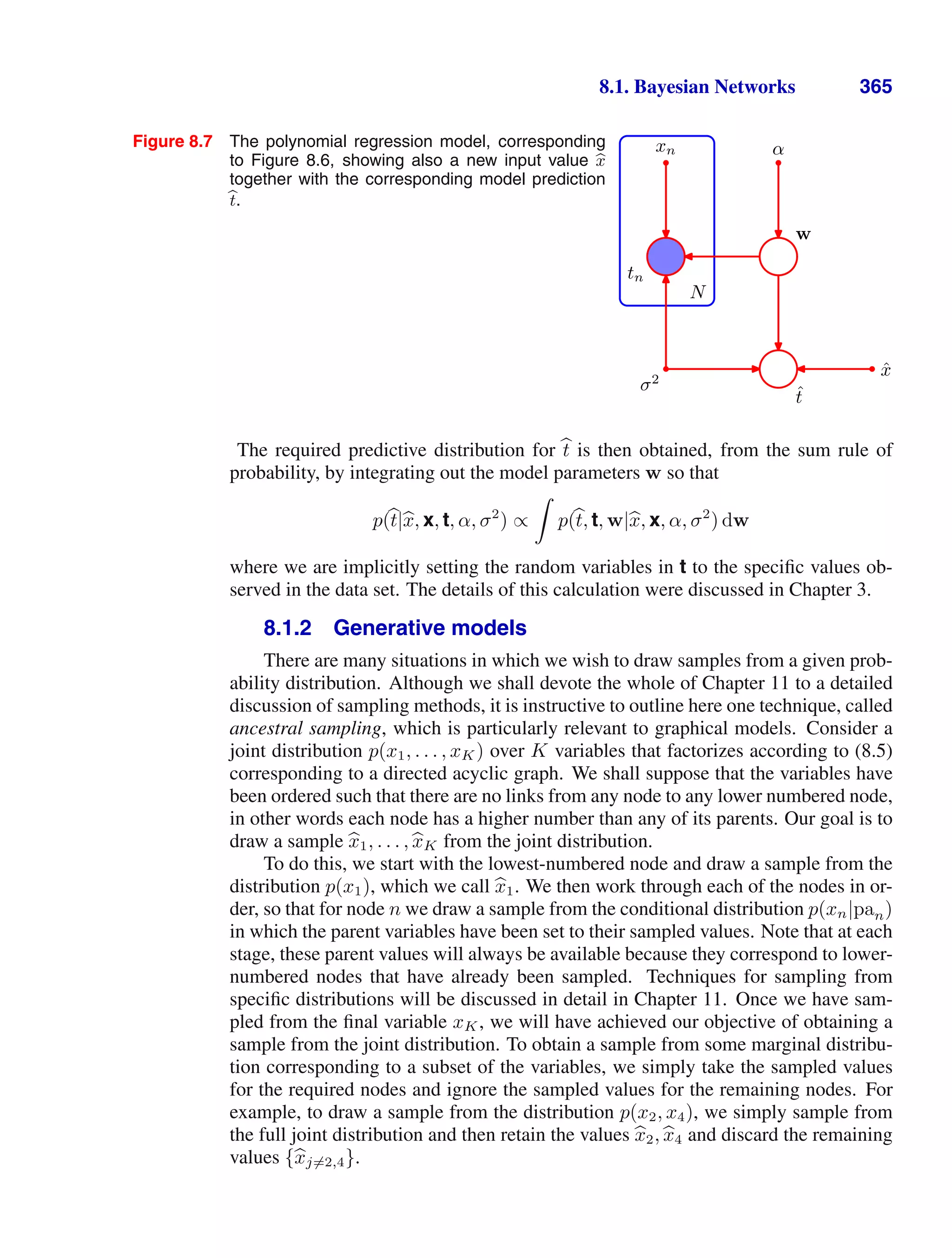
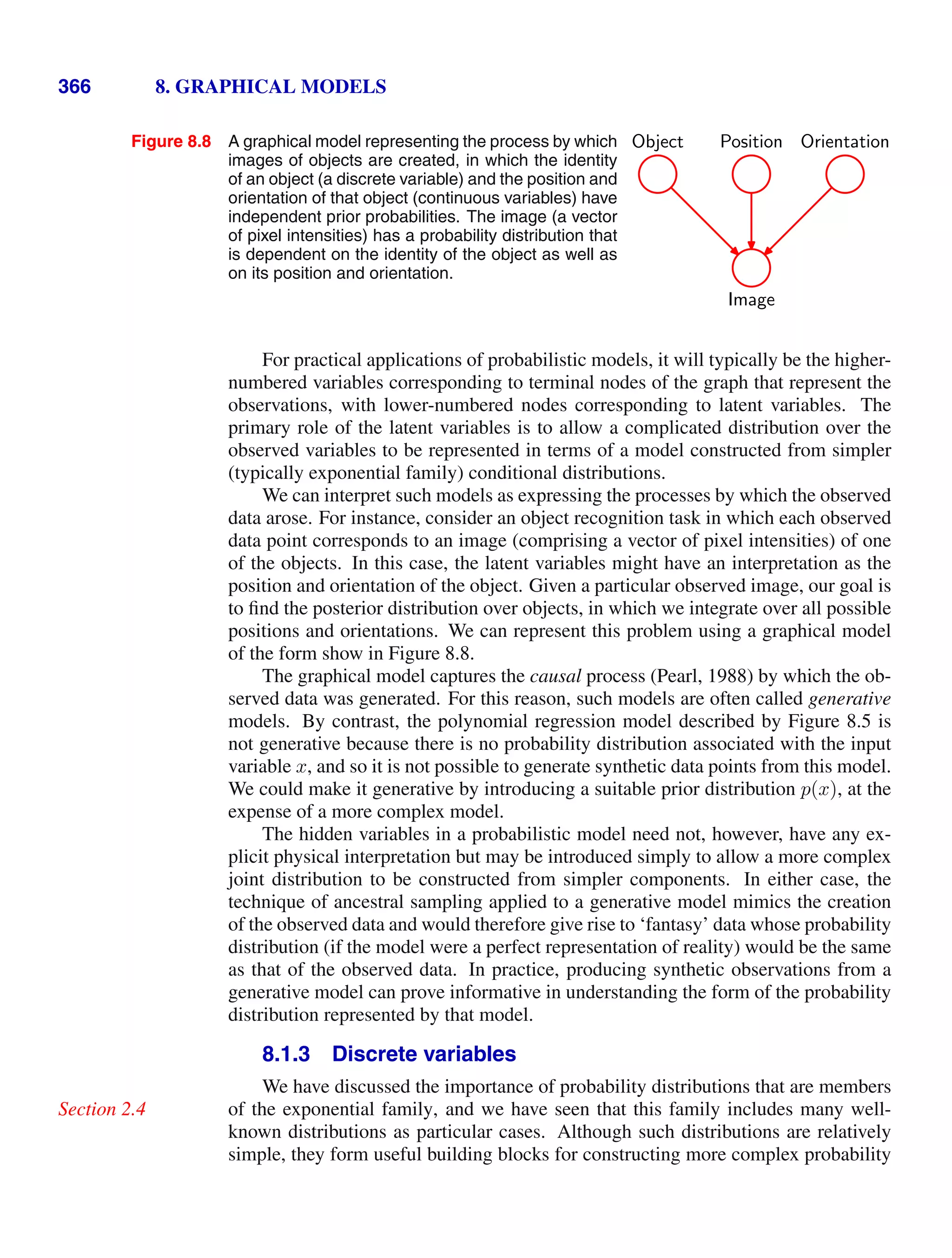
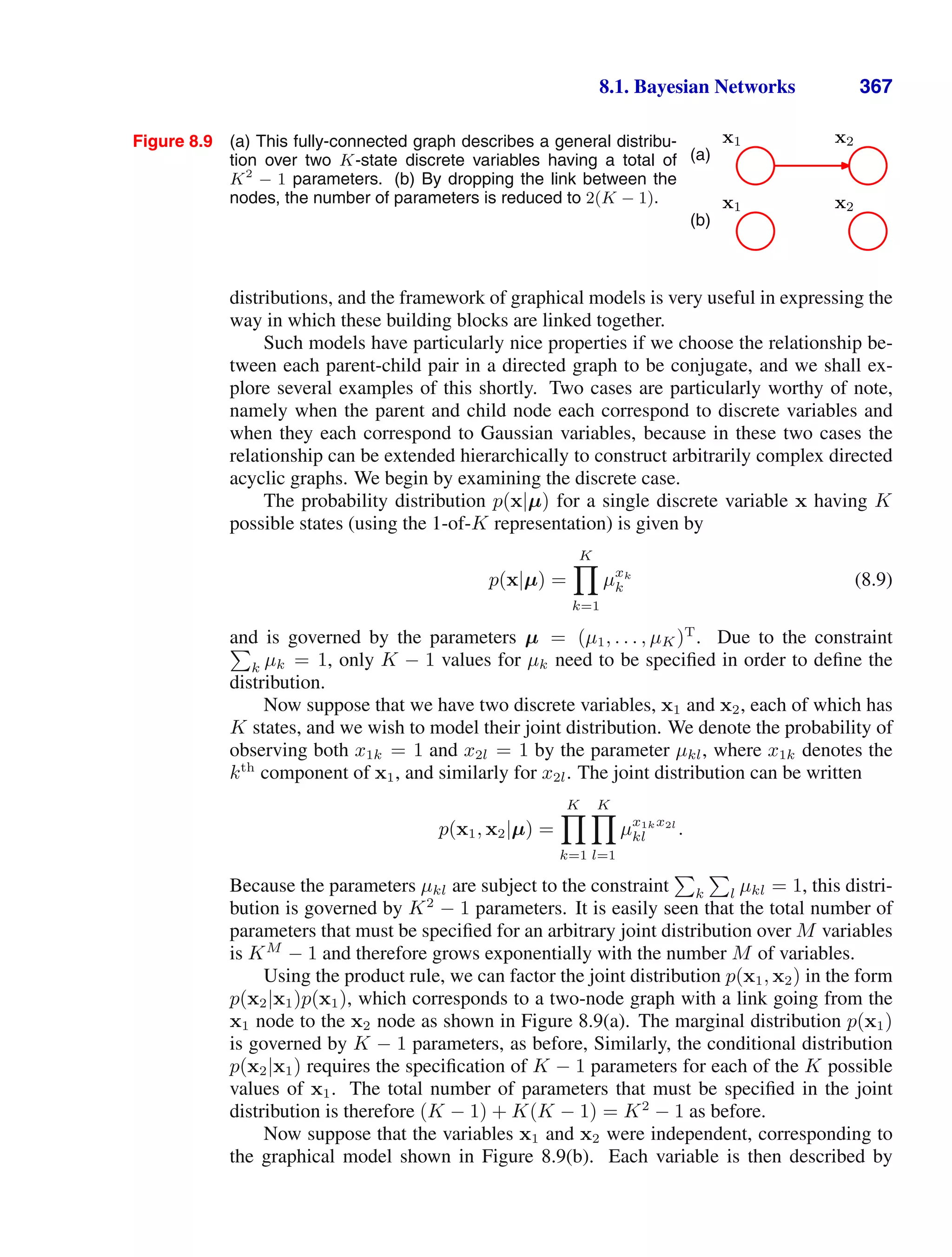
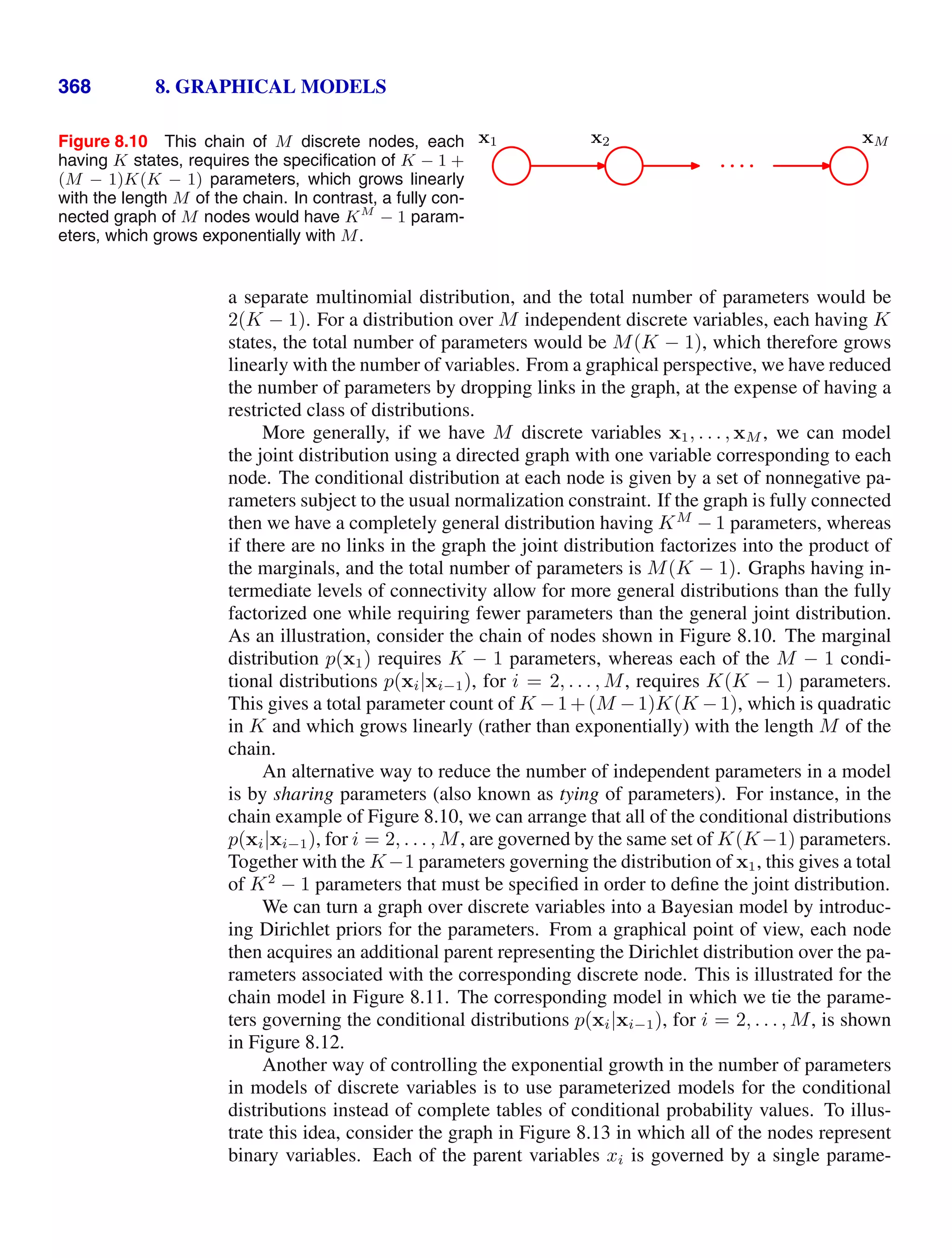
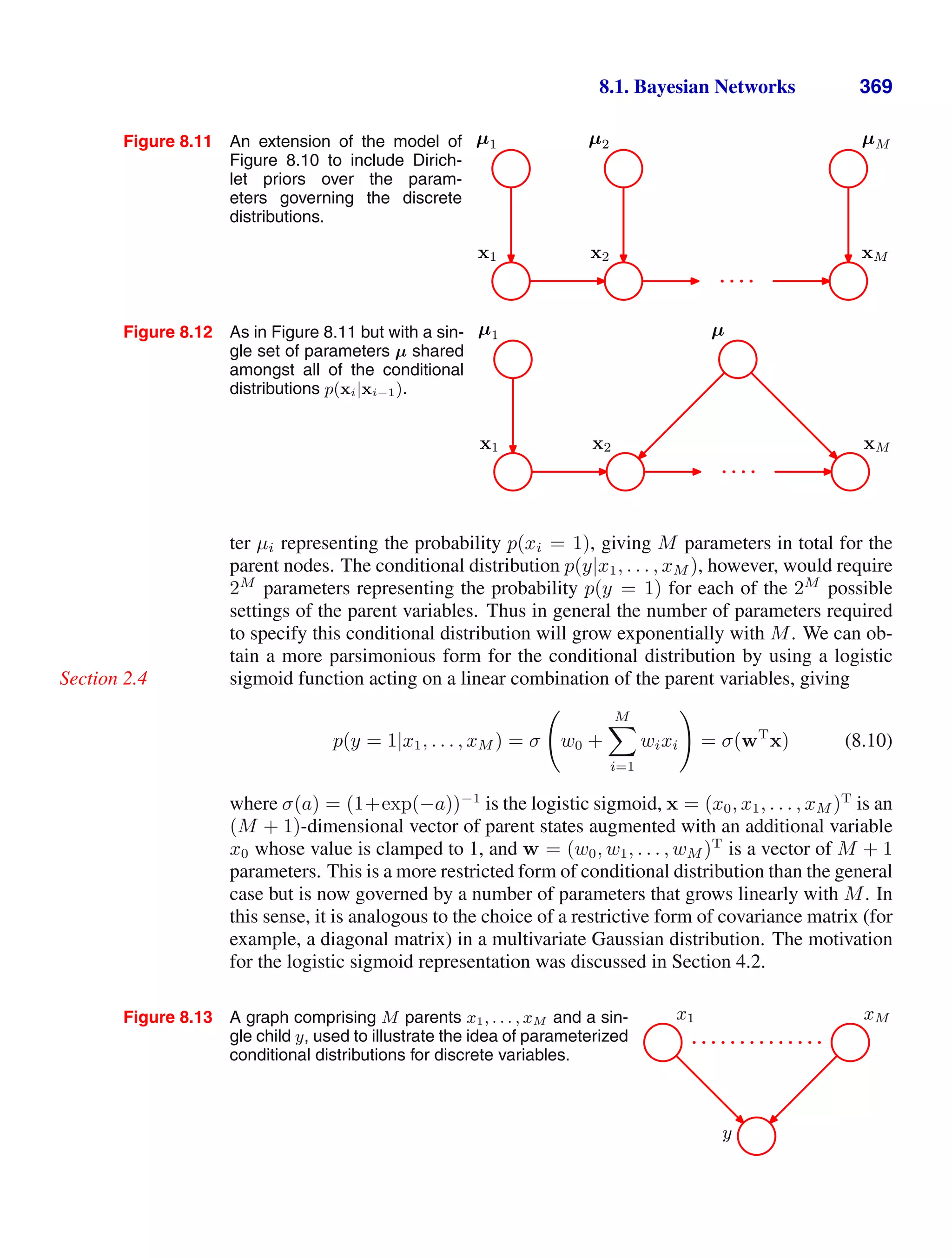
![370 8. GRAPHICAL MODELS
8.1.4 Linear-Gaussian models
In the previous section, we saw how to construct joint probability distributions
over a set of discrete variables by expressing the variables as nodes in a directed
acyclic graph. Here we show how a multivariate Gaussian can be expressed as a
directed graph corresponding to a linear-Gaussian model over the component vari-
ables. This allows us to impose interesting structure on the distribution, with the
general Gaussian and the diagonal covariance Gaussian representing opposite ex-
tremes. Several widely used techniques are examples of linear-Gaussian models,
such as probabilistic principal component analysis, factor analysis, and linear dy-
namical systems (Roweis and Ghahramani, 1999). We shall make extensive use of
the results of this section in later chapters when we consider some of these techniques
in detail.
Consider an arbitrary directed acyclic graph over D variables in which node i
represents a single continuous random variable xi having a Gaussian distribution.
The mean of this distribution is taken to be a linear combination of the states of its
parent nodes pai of node i
p(xi|pai) = N
⎛
⎝xi
j∈pai
wijxj + bi, vi
⎞
⎠ (8.11)
where wij and bi are parameters governing the mean, and vi is the variance of the
conditional distribution for xi. The log of the joint distribution is then the log of the
product of these conditionals over all nodes in the graph and hence takes the form
ln p(x) =
D
i=1
ln p(xi|pai) (8.12)
= −
D
i=1
1
2vi
⎛
⎝xi −
j∈pai
wijxj − bi
⎞
⎠
2
+ const (8.13)
where x = (x1, . . . , xD)T
and ‘const’ denotes terms independent of x. We see that
this is a quadratic function of the components of x, and hence the joint distribution
p(x) is a multivariate Gaussian.
We can determine the mean and covariance of the joint distribution recursively
as follows. Each variable xi has (conditional on the states of its parents) a Gaussian
distribution of the form (8.11) and so
xi =
j∈pai
wijxj + bi +
√
vii (8.14)
where i is a zero mean, unit variance Gaussian random variable satisfying E[i] = 0
and E[ij] = Iij, where Iij is the i, j element of the identity matrix. Taking the
expectation of (8.14), we have
E[xi] =
j∈pai
wijE[xj] + bi. (8.15)](https://image.slidesharecdn.com/bishop-patternrecognitionandmachinelearning-230316082240-9af1cdaa/75/Bishop-Pattern-Recognition-and-Machine-Learning-pdf-386-2048.jpg)
![8.1. Bayesian Networks 371
Figure 8.14 A directed graph over three Gaussian variables,
with one missing link.
x1 x2 x3
Thus we can find the components of E[x] = (E[x1], . . . , E[xD])T
by starting at the
lowest numbered node and working recursively through the graph (here we again
assume that the nodes are numbered such that each node has a higher number than
its parents). Similarly, we can use (8.14) and (8.15) to obtain the i, j element of the
covariance matrix for p(x) in the form of a recursion relation
cov[xi, xj] = E [(xi − E[xi])(xj − E[xj])]
= E
⎡
⎣(xi − E[xi])
⎧
⎨
⎩
k∈paj
wjk(xk − E[xk]) +
√
vjj
⎫
⎬
⎭
⎤
⎦
=
k∈paj
wjkcov[xi, xk] + Iijvj (8.16)
and so the covariance can similarly be evaluated recursively starting from the lowest
numbered node.
Let us consider two extreme cases. First of all, suppose that there are no links
in the graph, which therefore comprises D isolated nodes. In this case, there are no
parameters wij and so there are just D parameters bi and D parameters vi. From
the recursion relations (8.15) and (8.16), we see that the mean of p(x) is given by
(b1, . . . , bD)T
and the covariance matrix is diagonal of the form diag(v1, . . . , vD).
The joint distribution has a total of 2D parameters and represents a set of D inde-
pendent univariate Gaussian distributions.
Now consider a fully connected graph in which each node has all lower num-
bered nodes as parents. The matrix wij then has i − 1 entries on the ith
row and
hence is a lower triangular matrix (with no entries on the leading diagonal). Then
the total number of parameters wij is obtained by taking the number D2
of elements
in a D ×D matrix, subtracting D to account for the absence of elements on the lead-
ing diagonal, and then dividing by 2 because the matrix has elements only below the
diagonal, giving a total of D(D−1)/2. The total number of independent parameters
{wij} and {vi} in the covariance matrix is therefore D(D + 1)/2 corresponding to
a general symmetric covariance matrix.
Section 2.3
Graphs having some intermediate level of complexity correspond to joint Gaus-
sian distributions with partially constrained covariance matrices. Consider for ex-
ample the graph shown in Figure 8.14, which has a link missing between variables
x1 and x3. Using the recursion relations (8.15) and (8.16), we see that the mean and
covariance of the joint distribution are given by
Exercise 8.7
µ = (b1, b2 + w21b1, b3 + w32b2 + w32w21b1)
T
(8.17)
Σ =
v1 w21v1 w32w21v1
w21v1 v2 + w2
21v1 w32(v2 + w2
21v1)
w32w21v1 w32(v2 + w2
21v1) v3 + w2
32(v2 + w2
21v1)
. (8.18)](https://image.slidesharecdn.com/bishop-patternrecognitionandmachinelearning-230316082240-9af1cdaa/75/Bishop-Pattern-Recognition-and-Machine-Learning-pdf-387-2048.jpg)
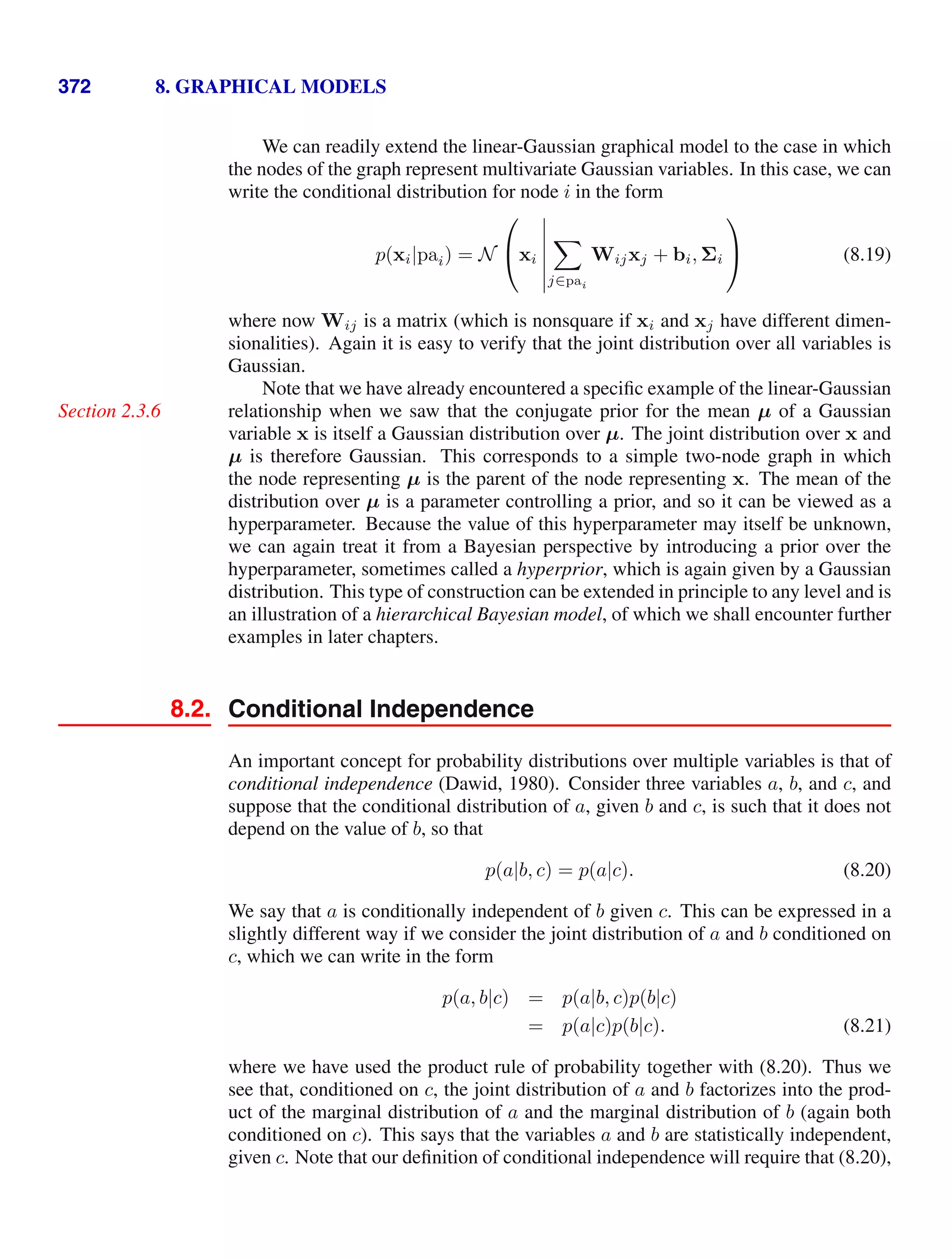
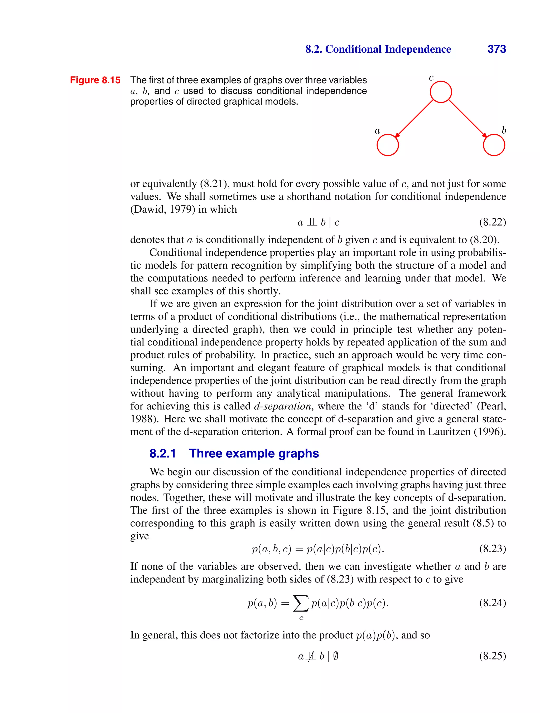
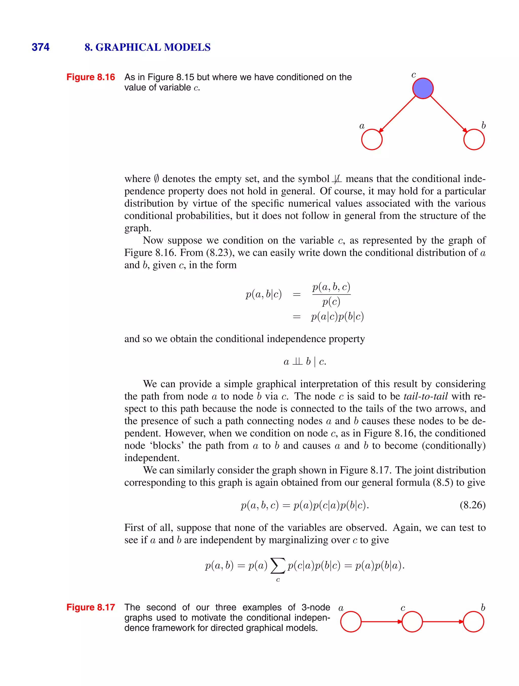
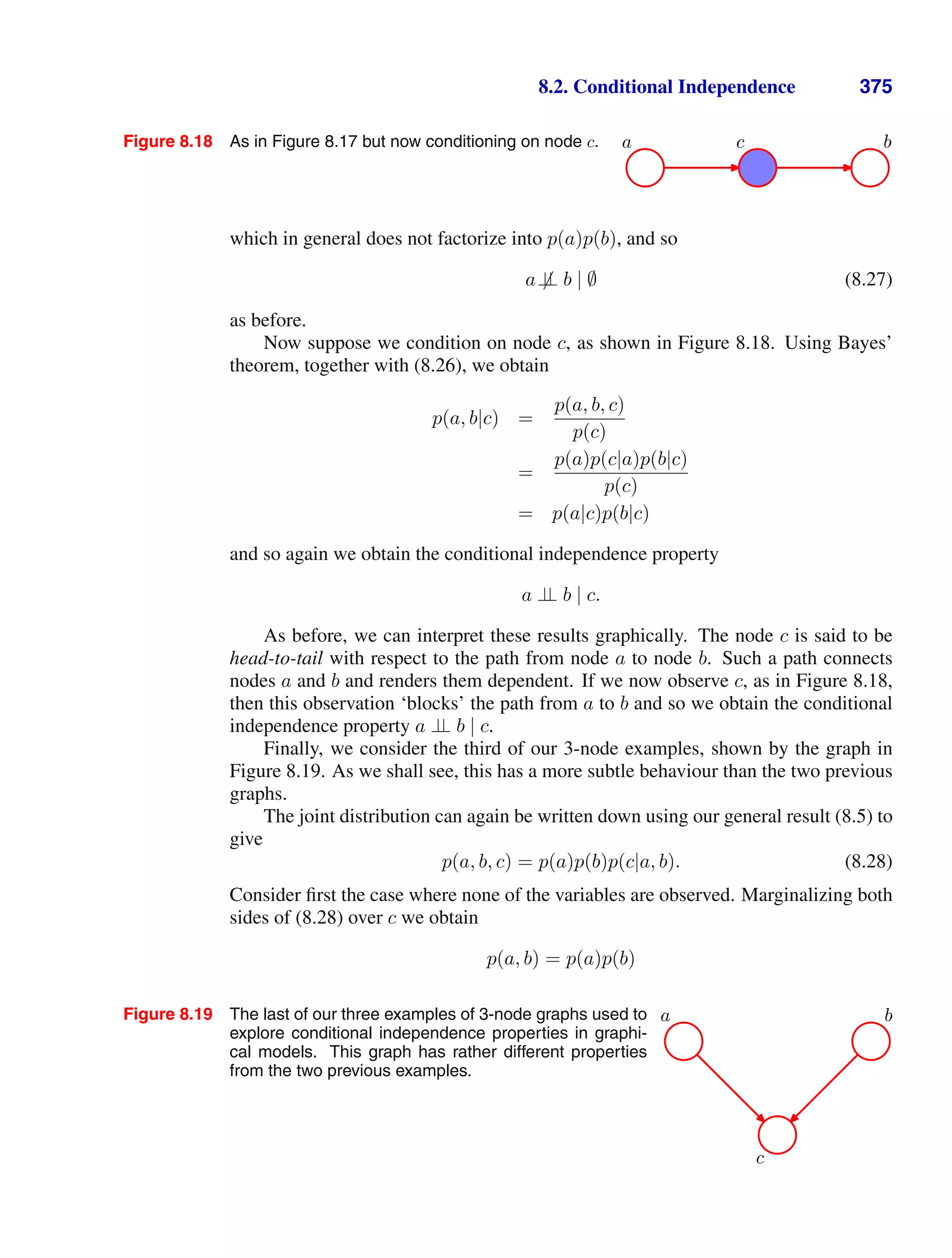
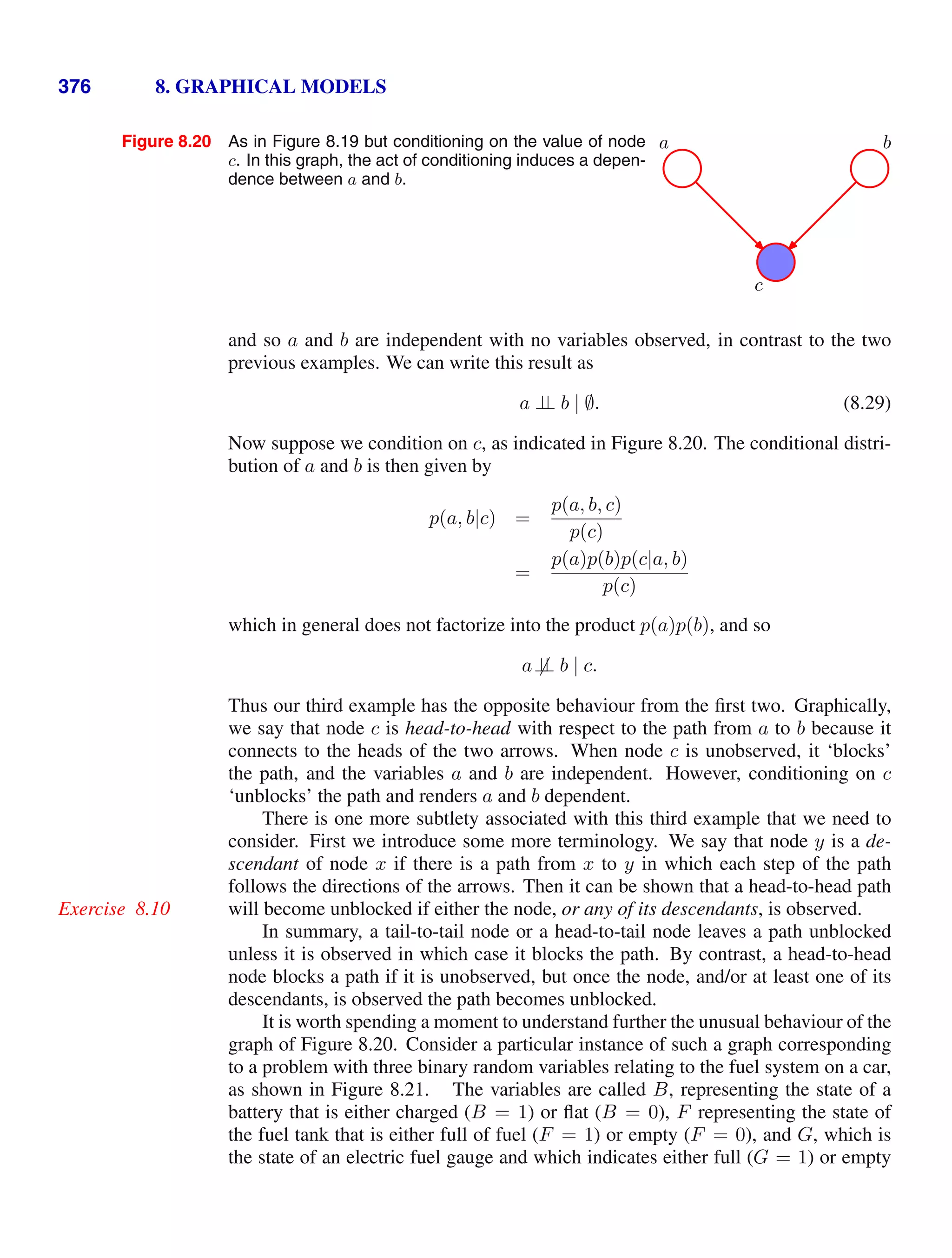
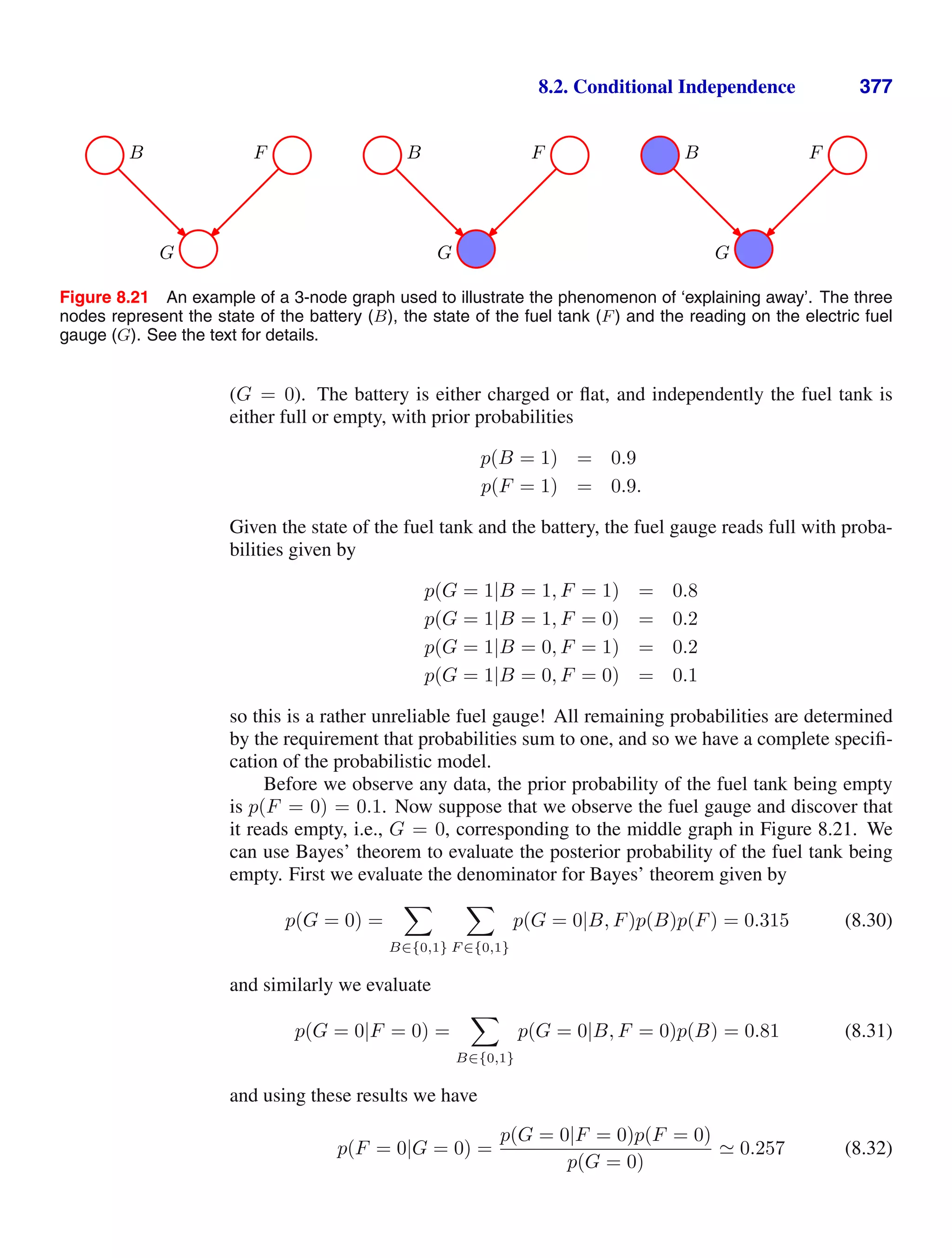
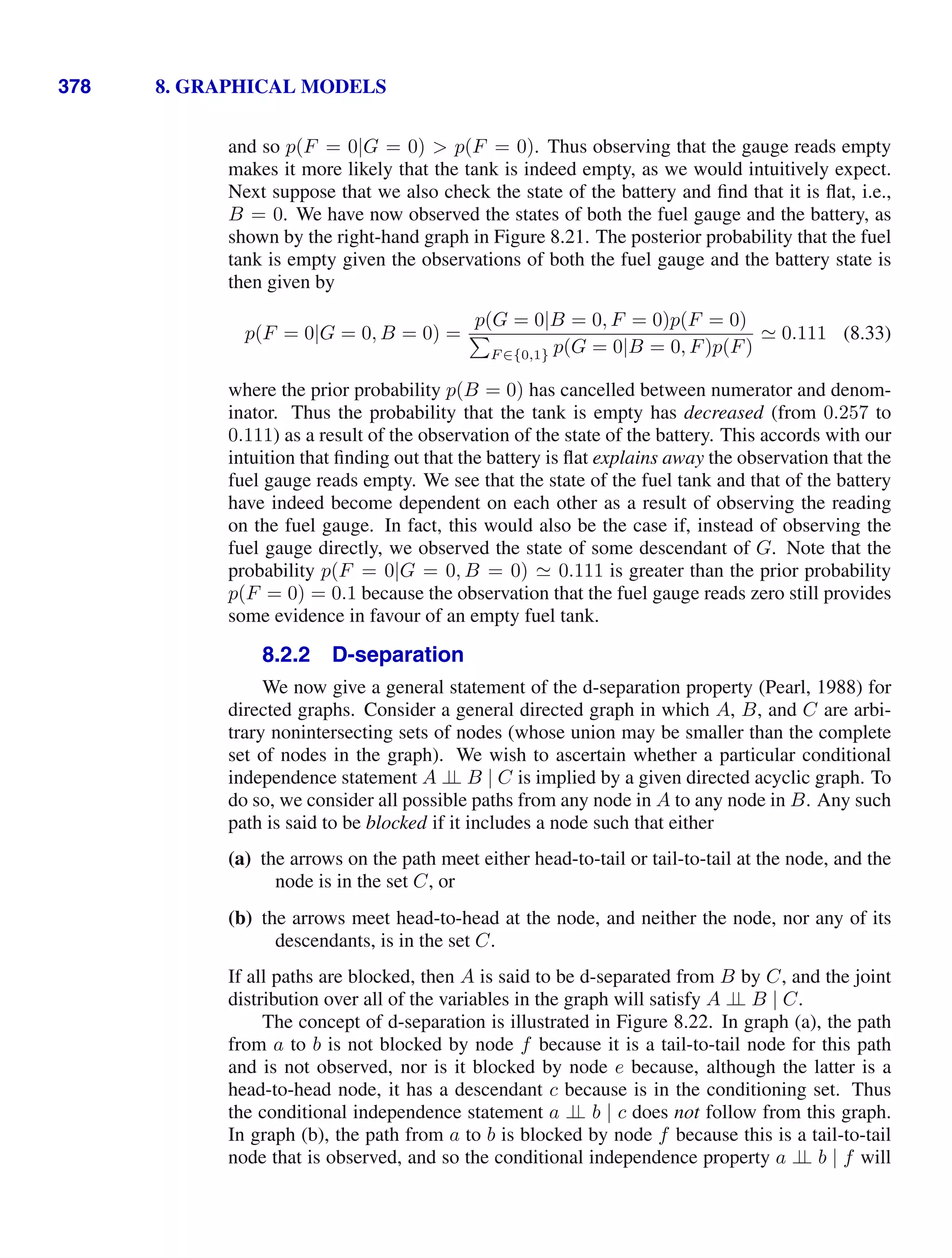
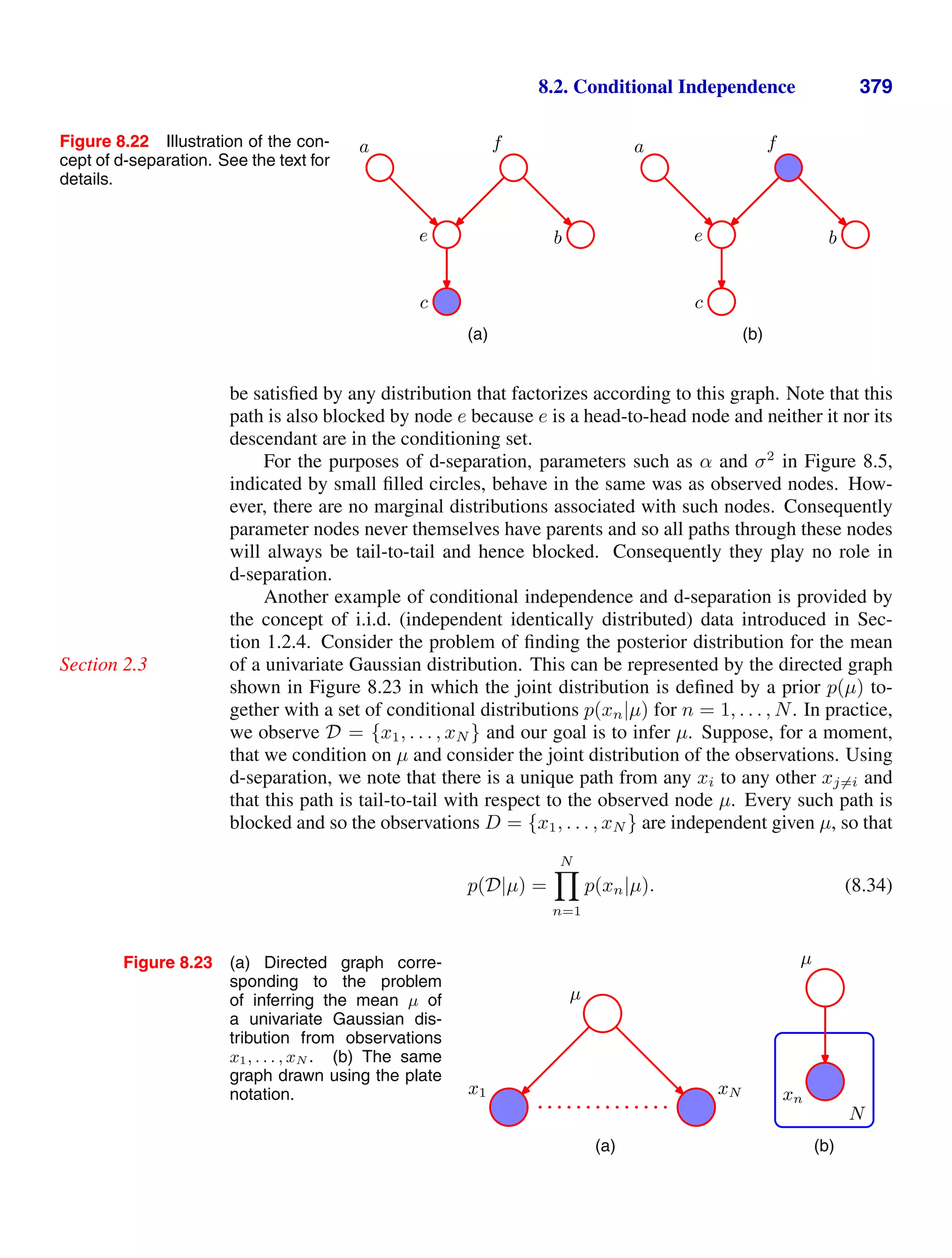
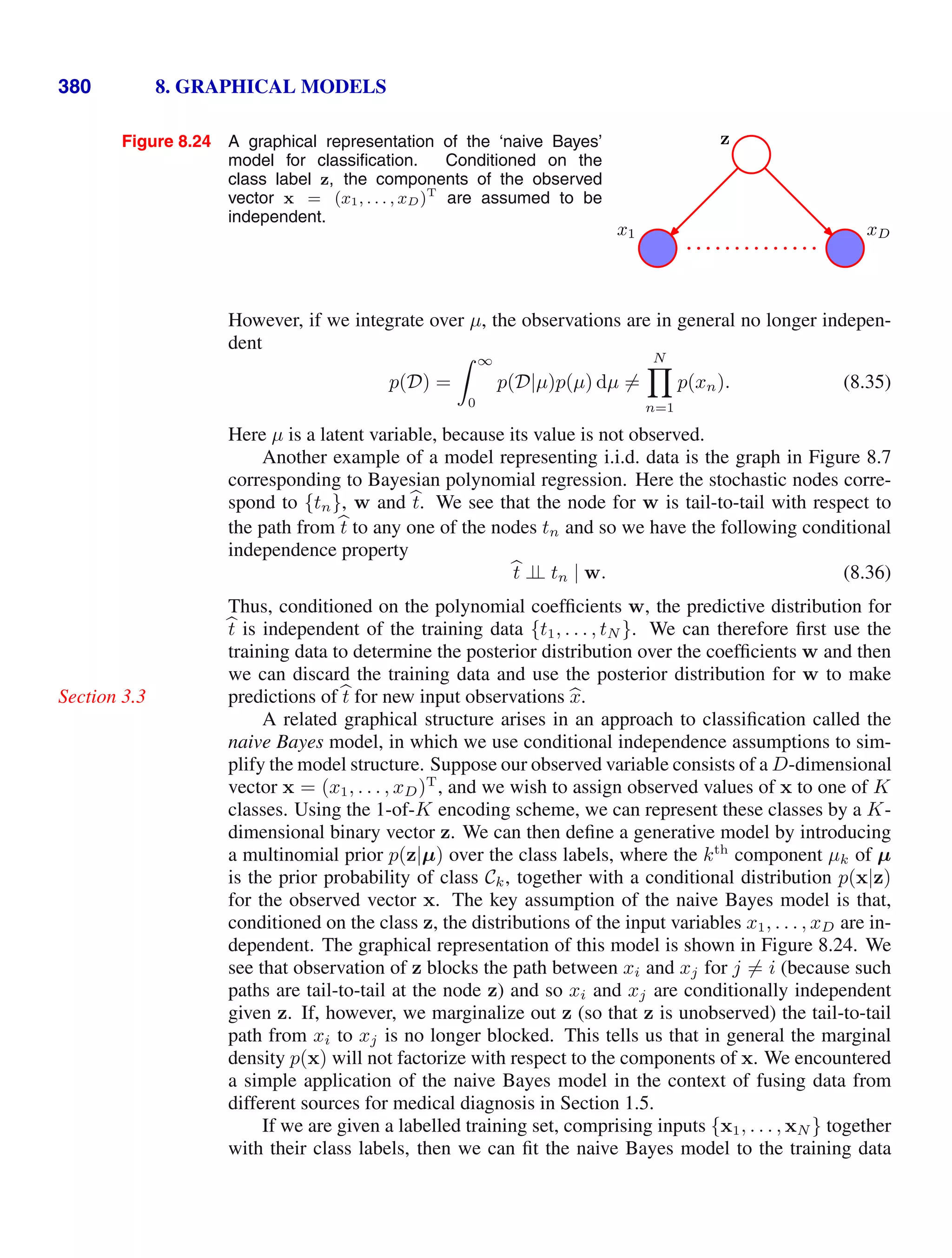
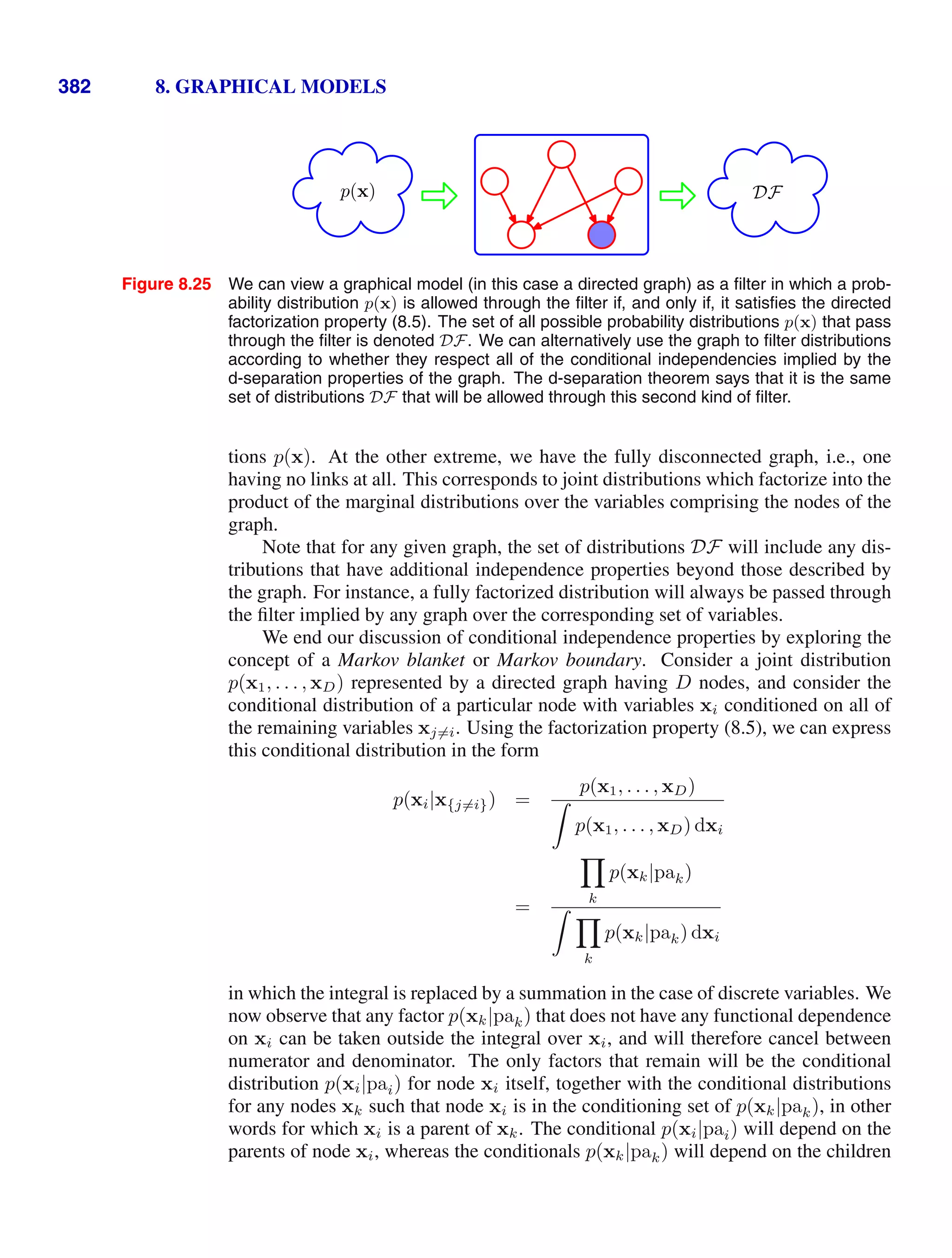
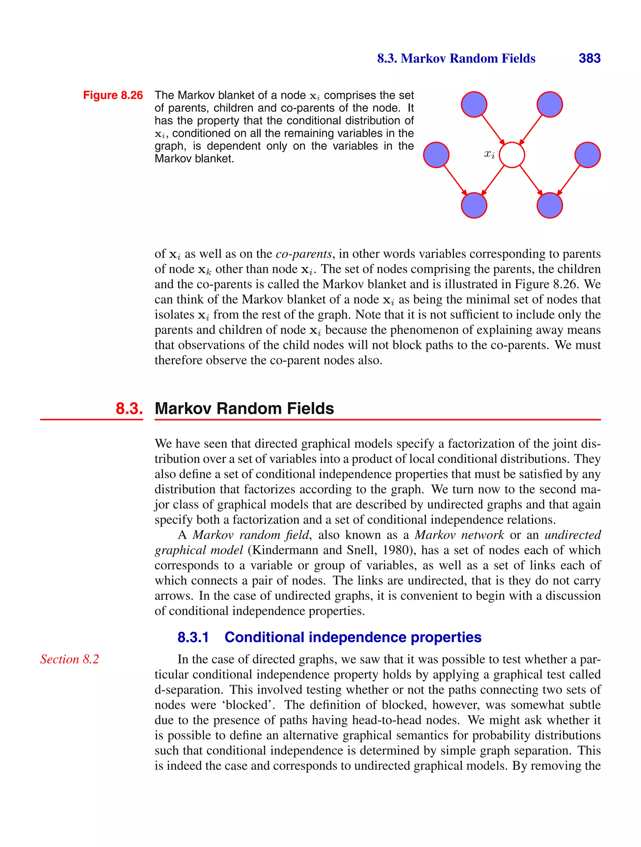
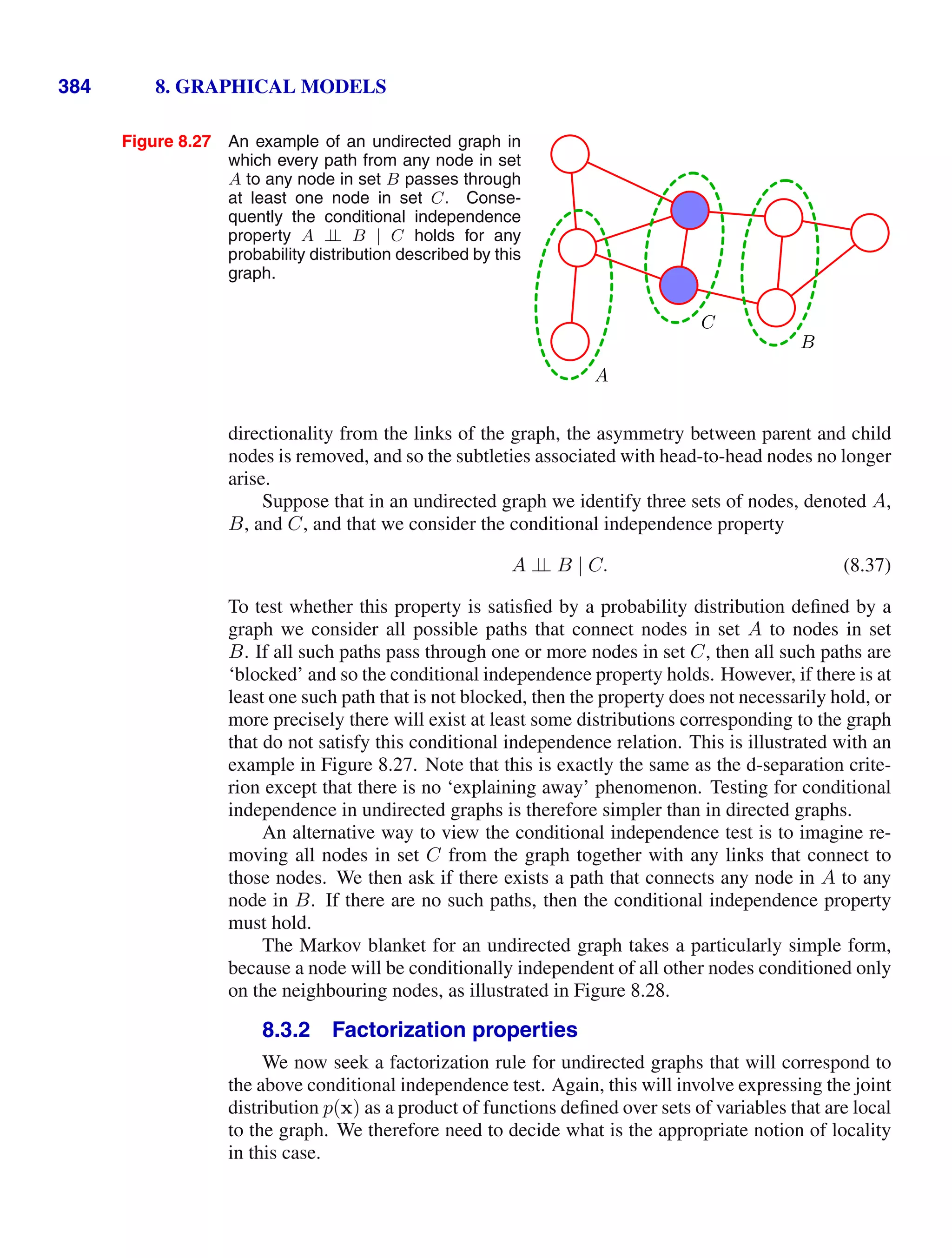
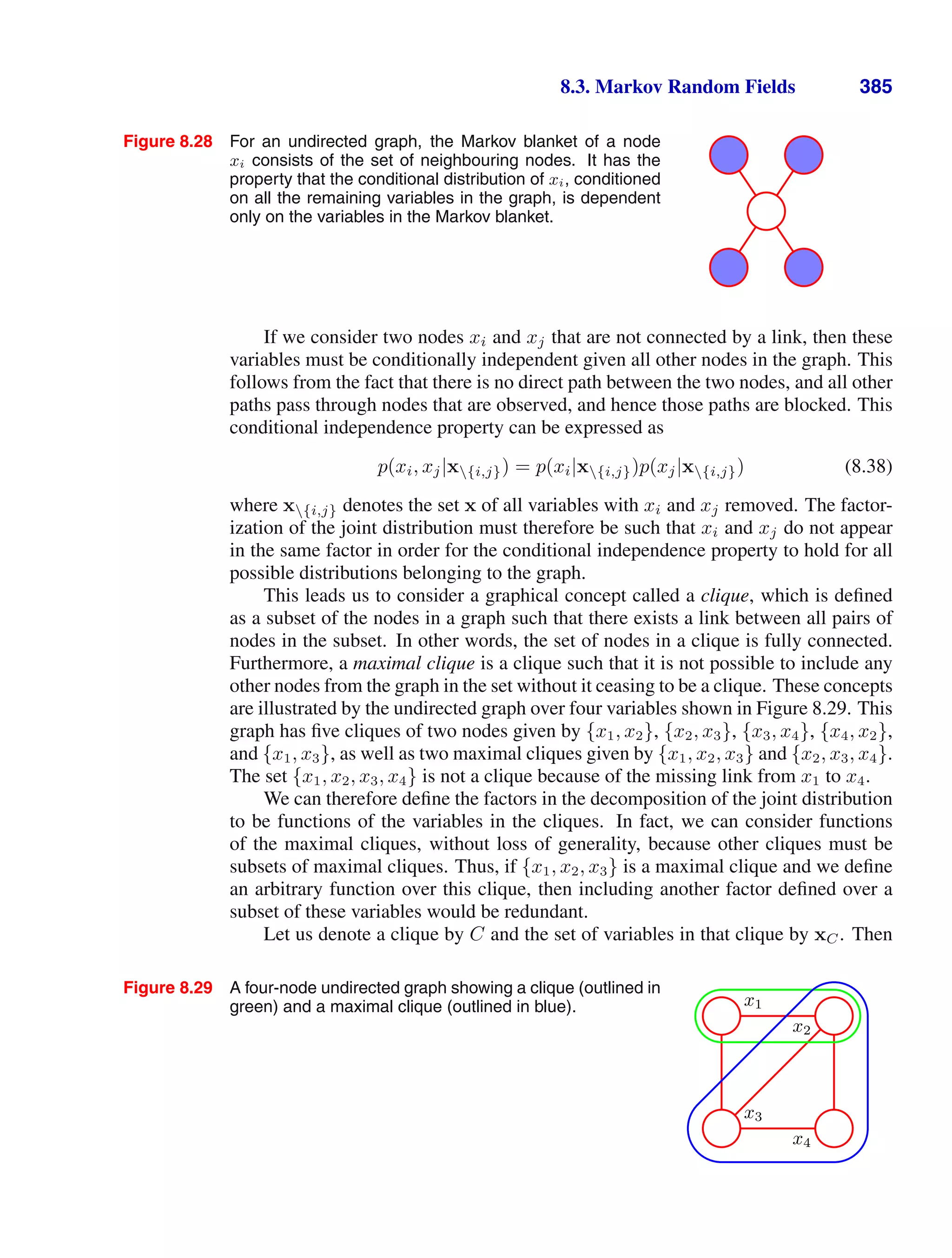
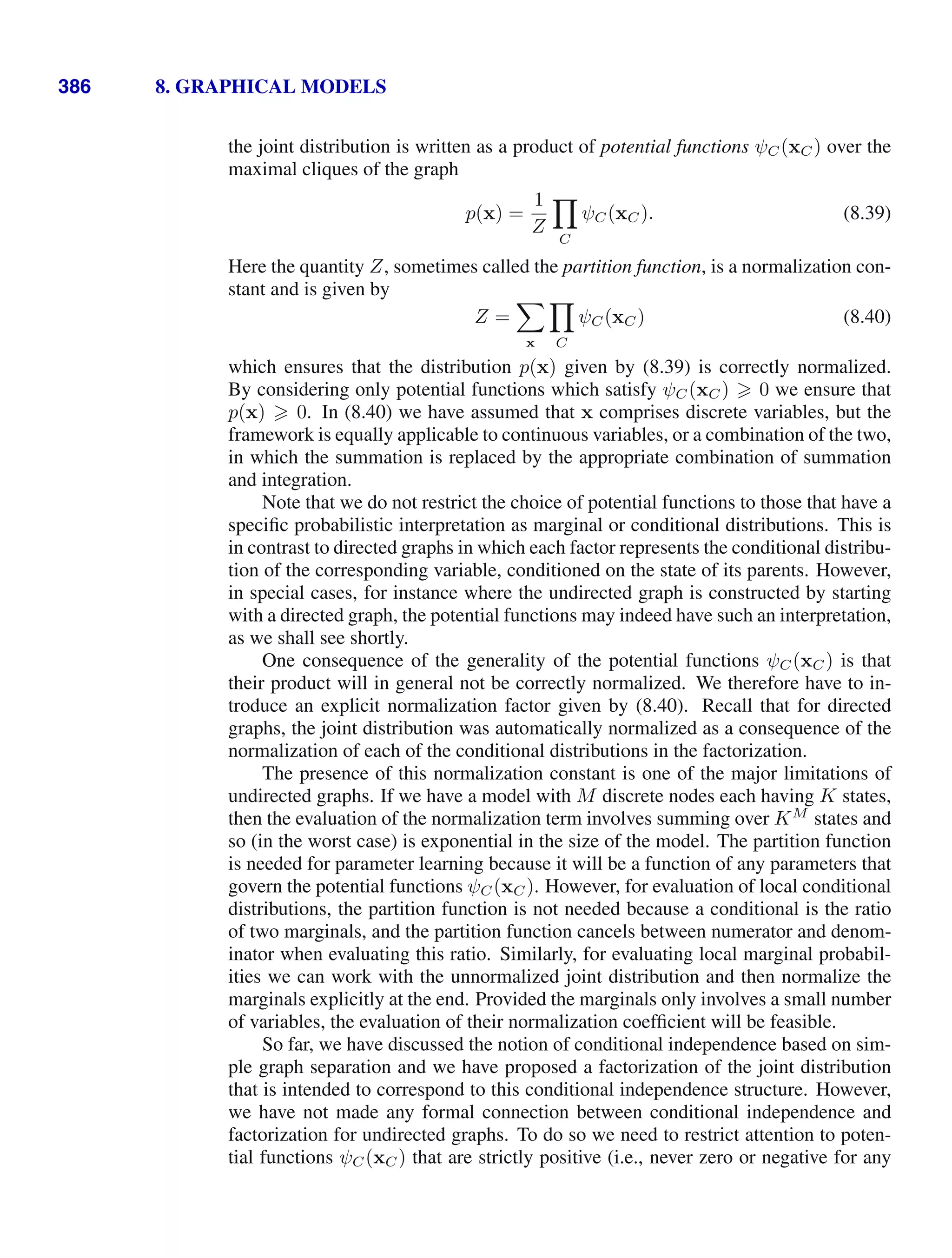
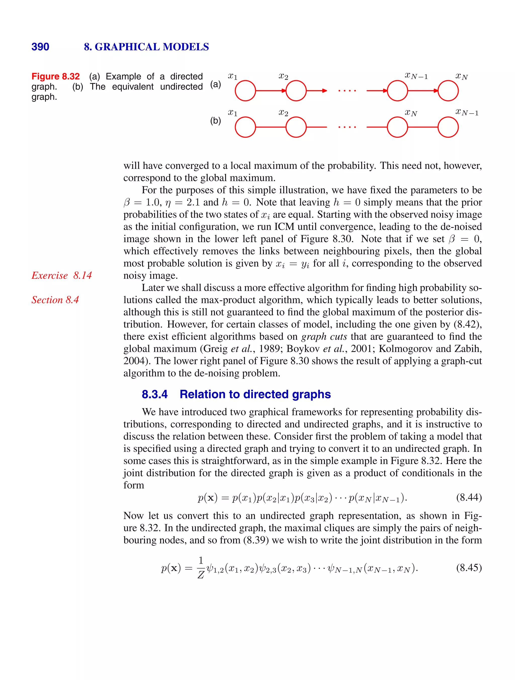
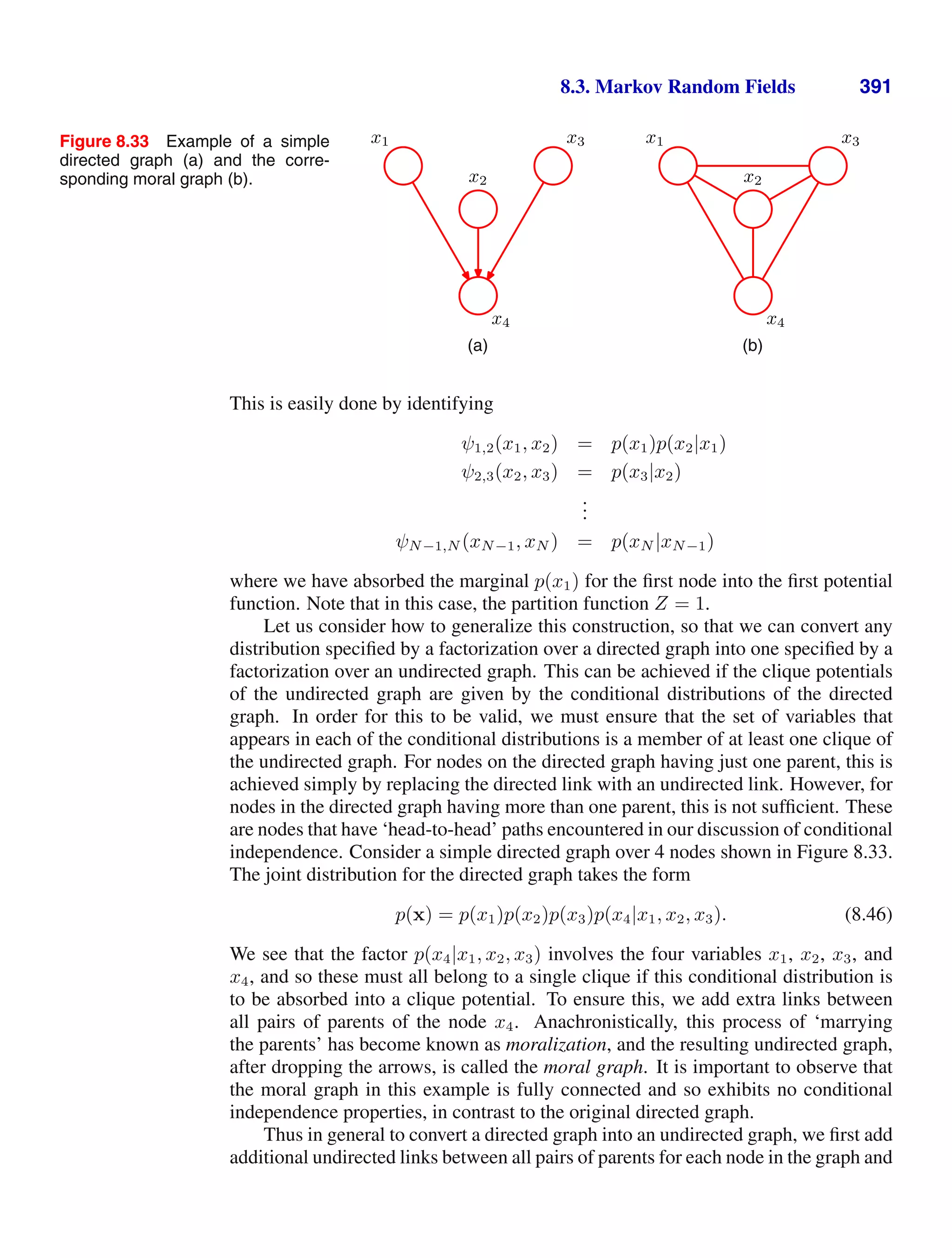
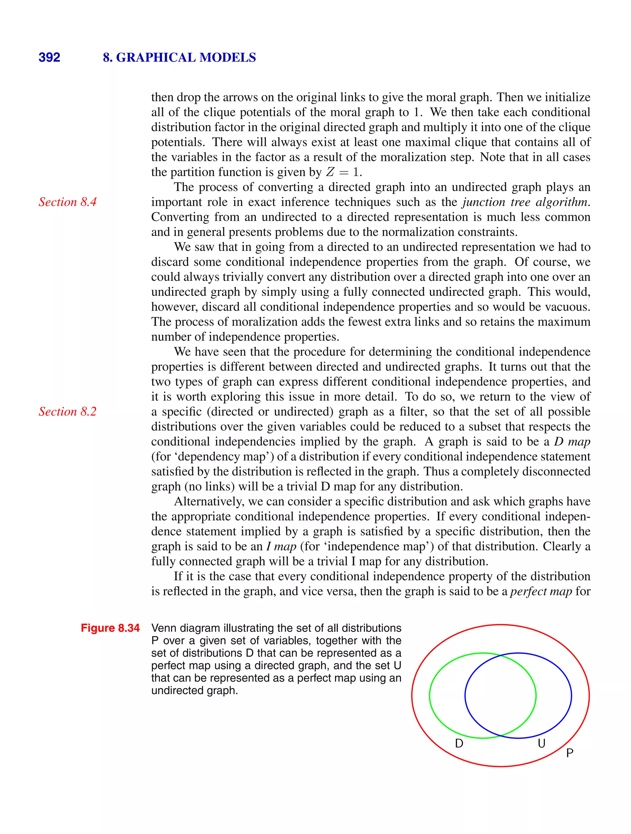
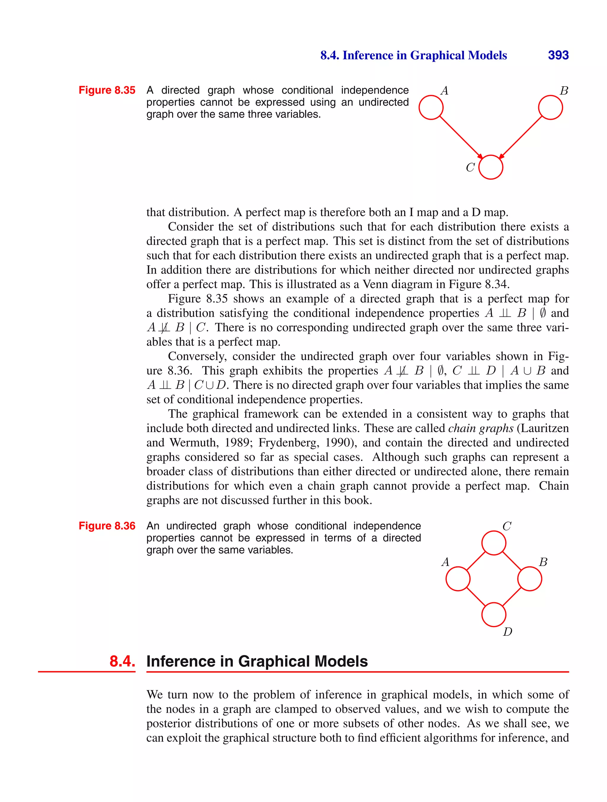
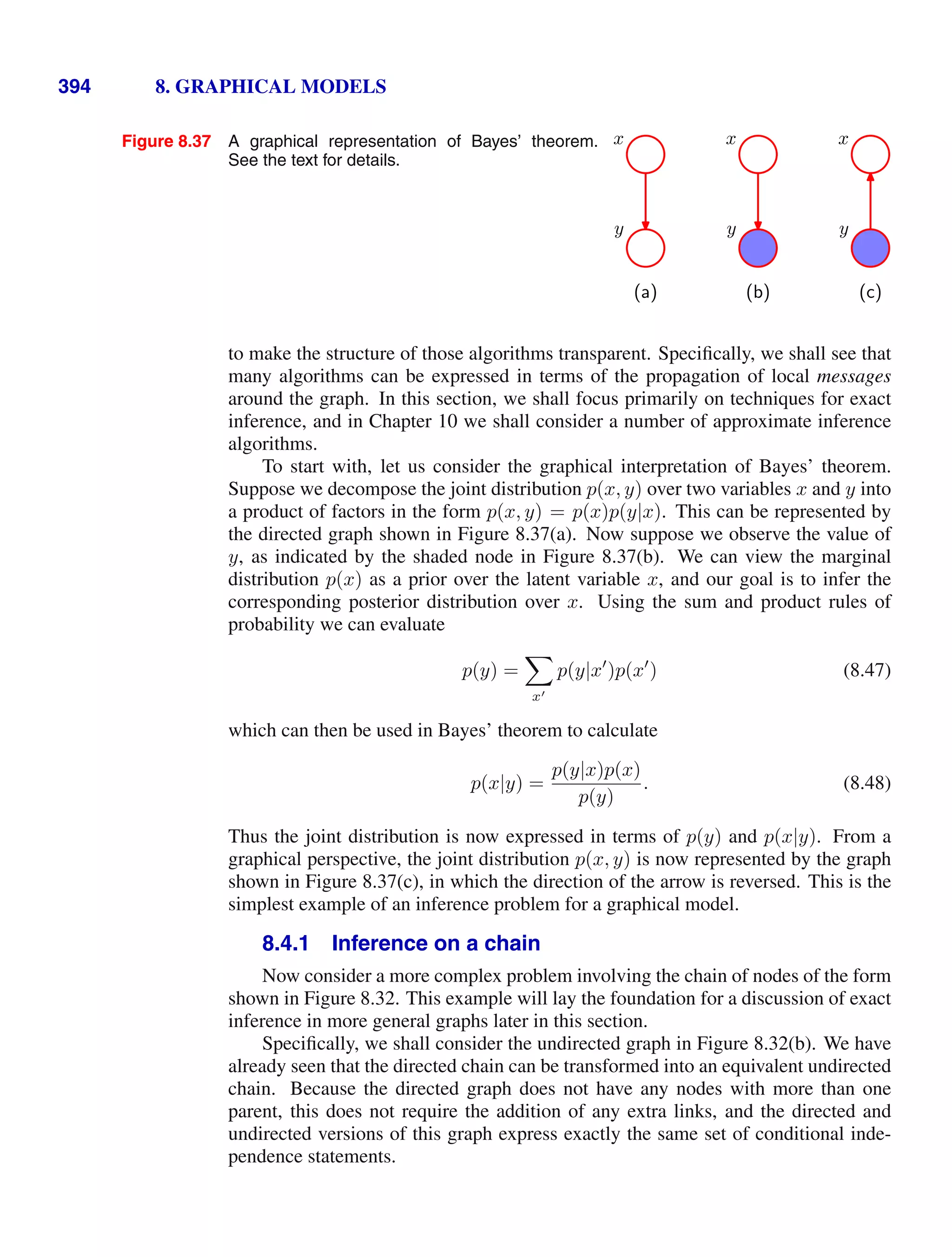
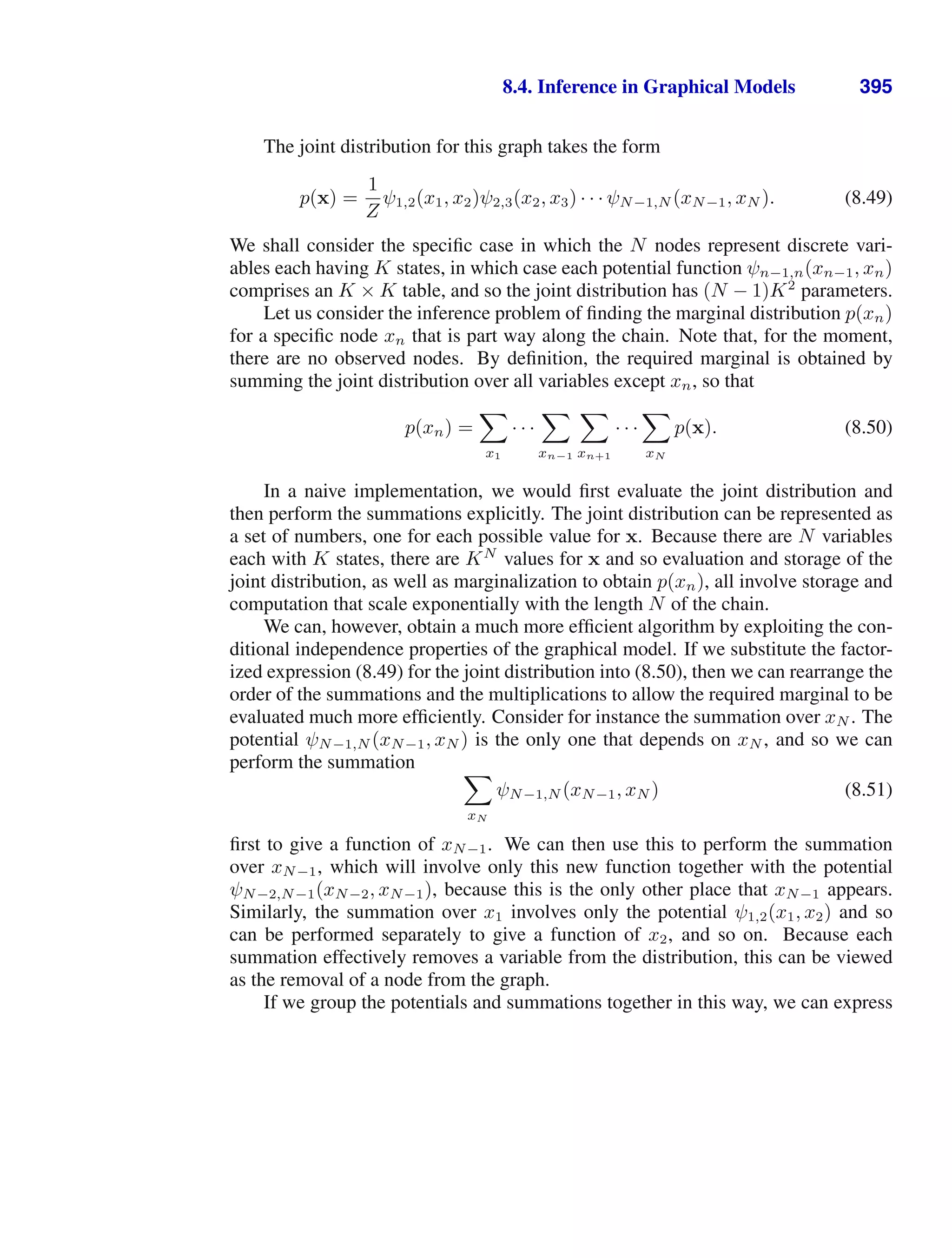
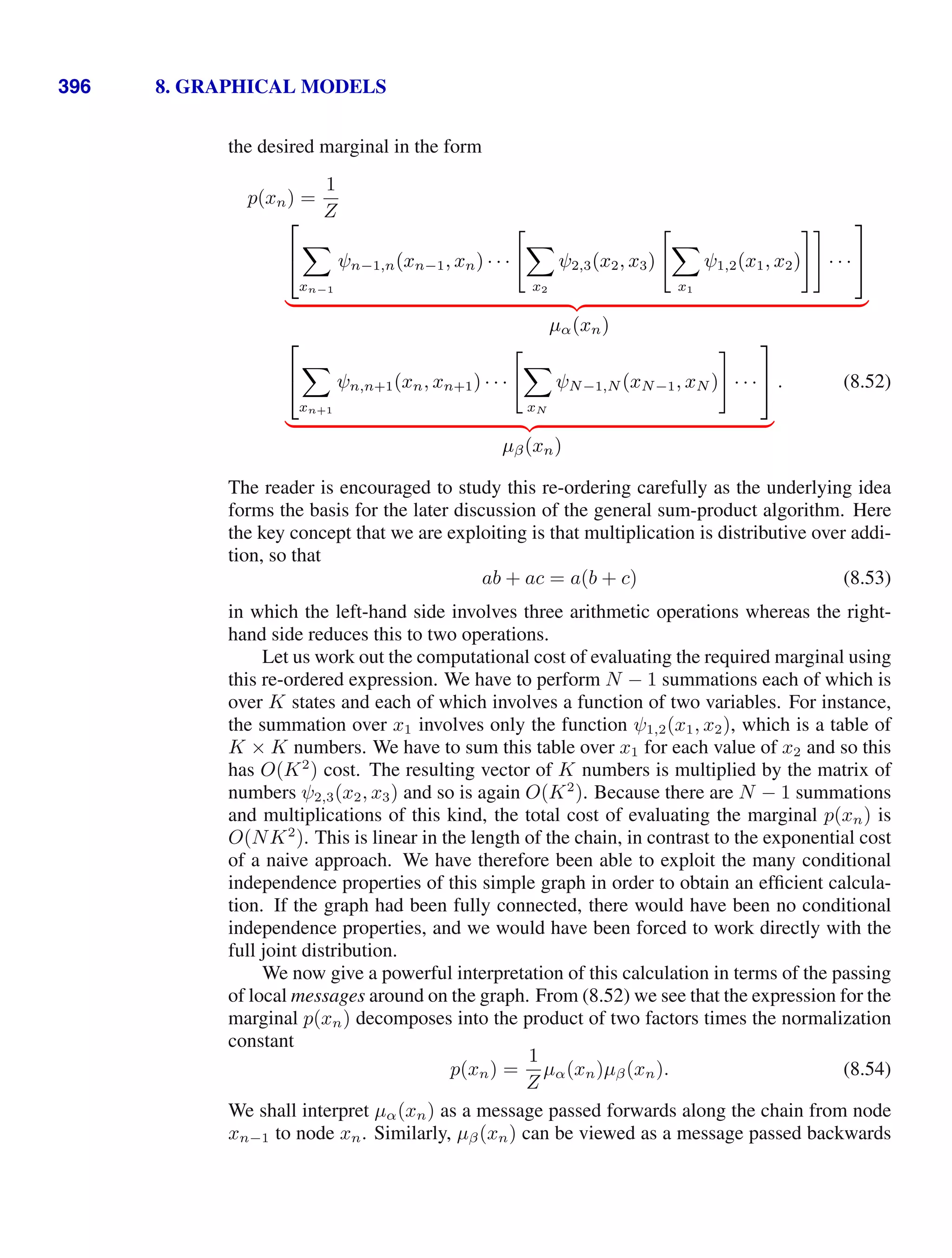
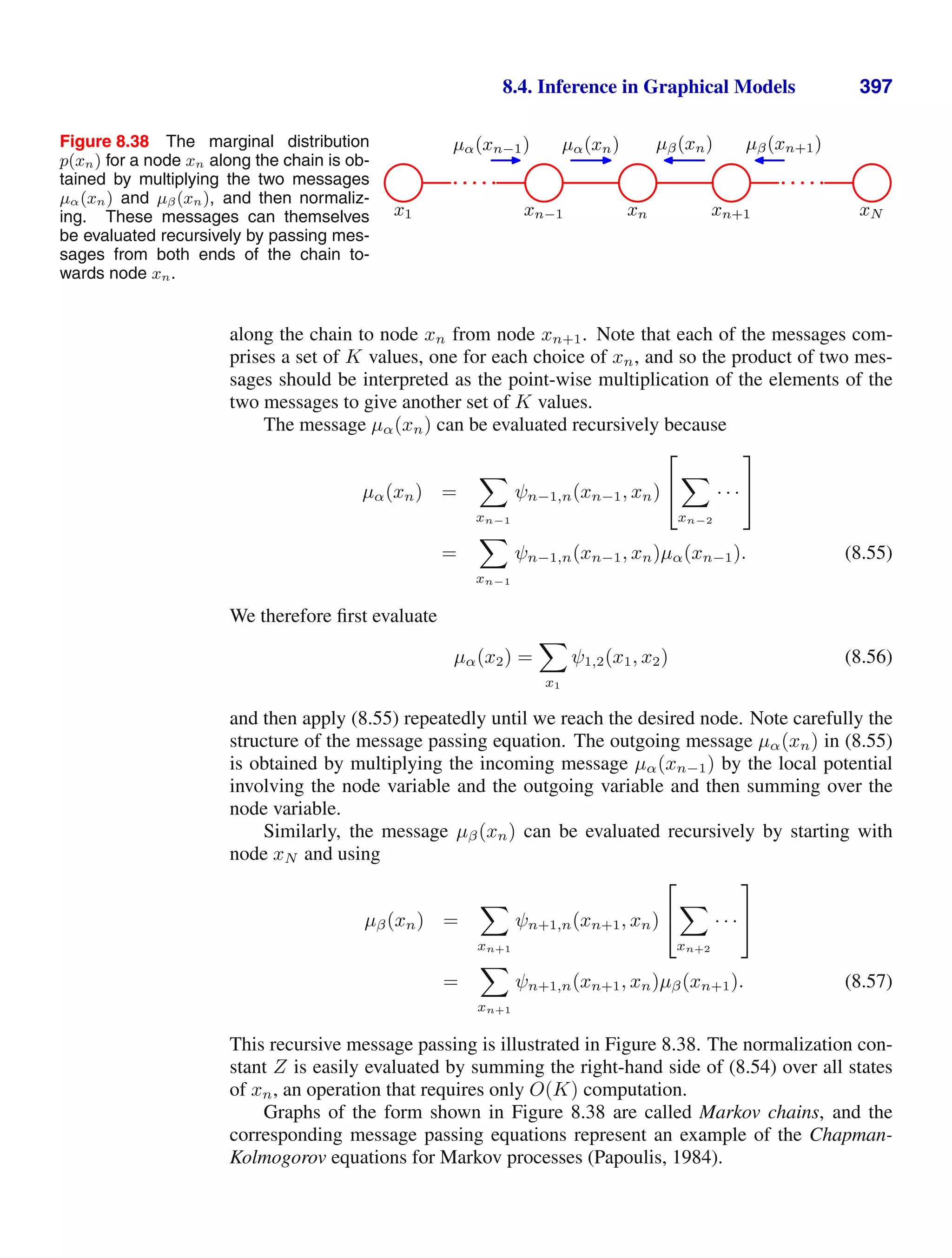
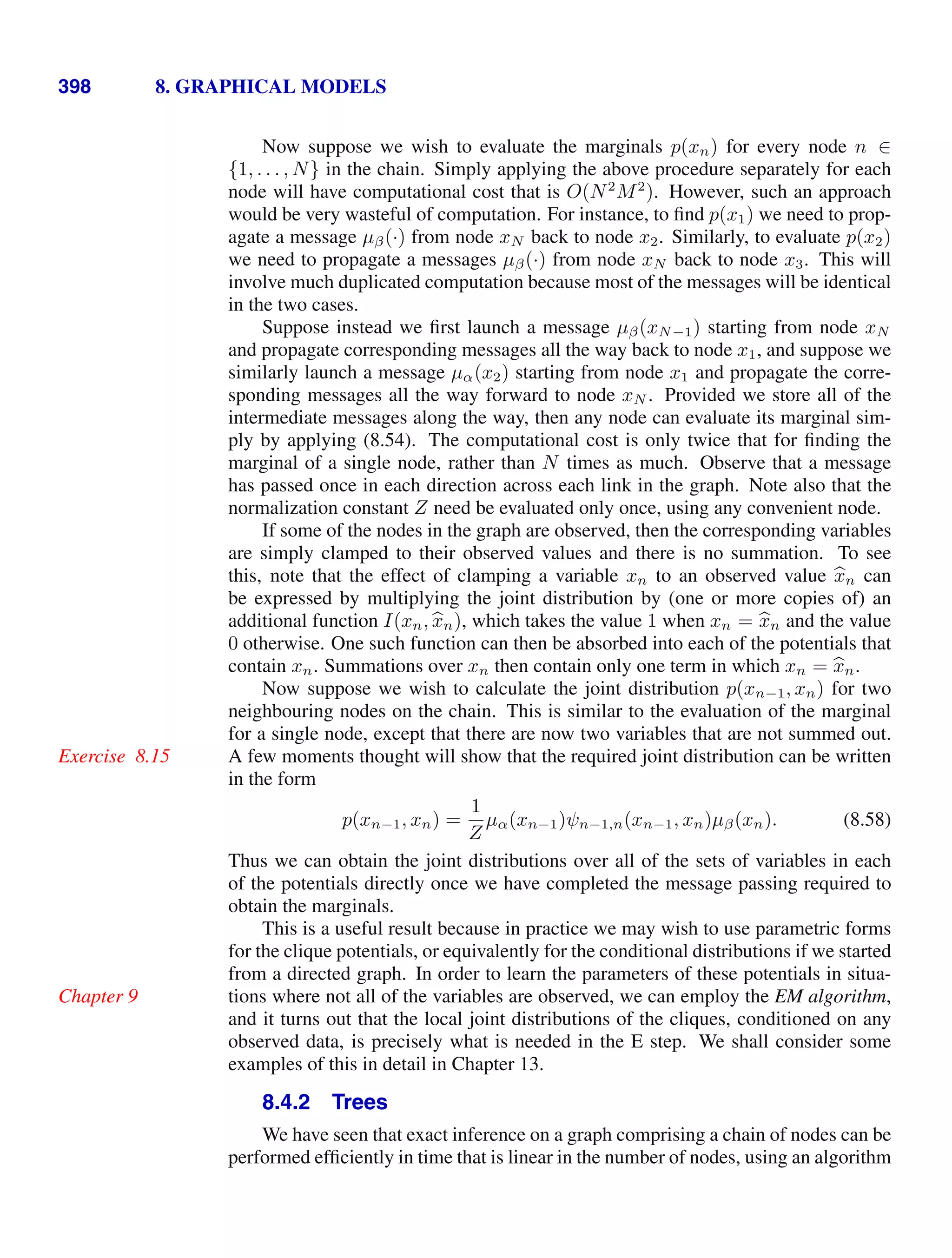
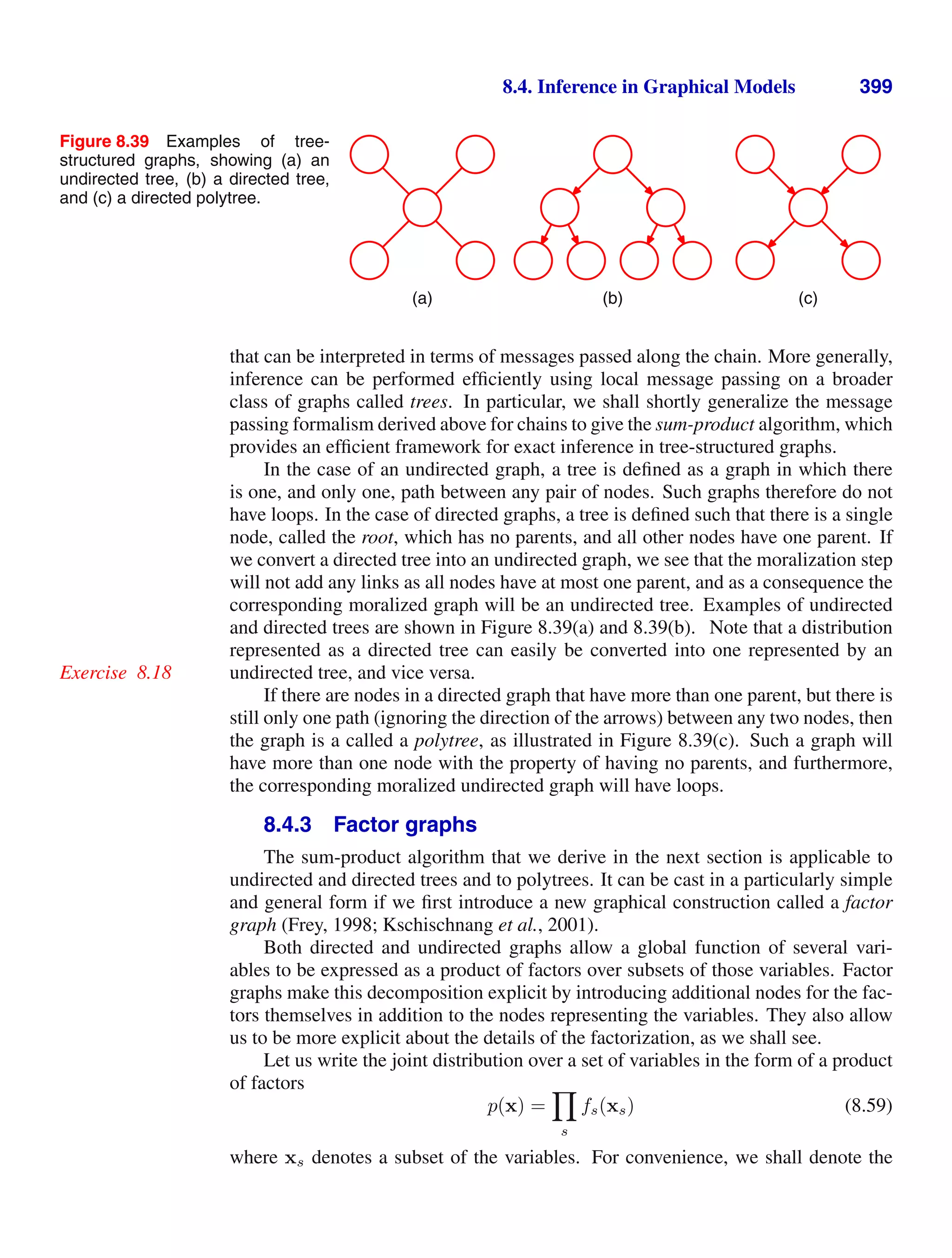
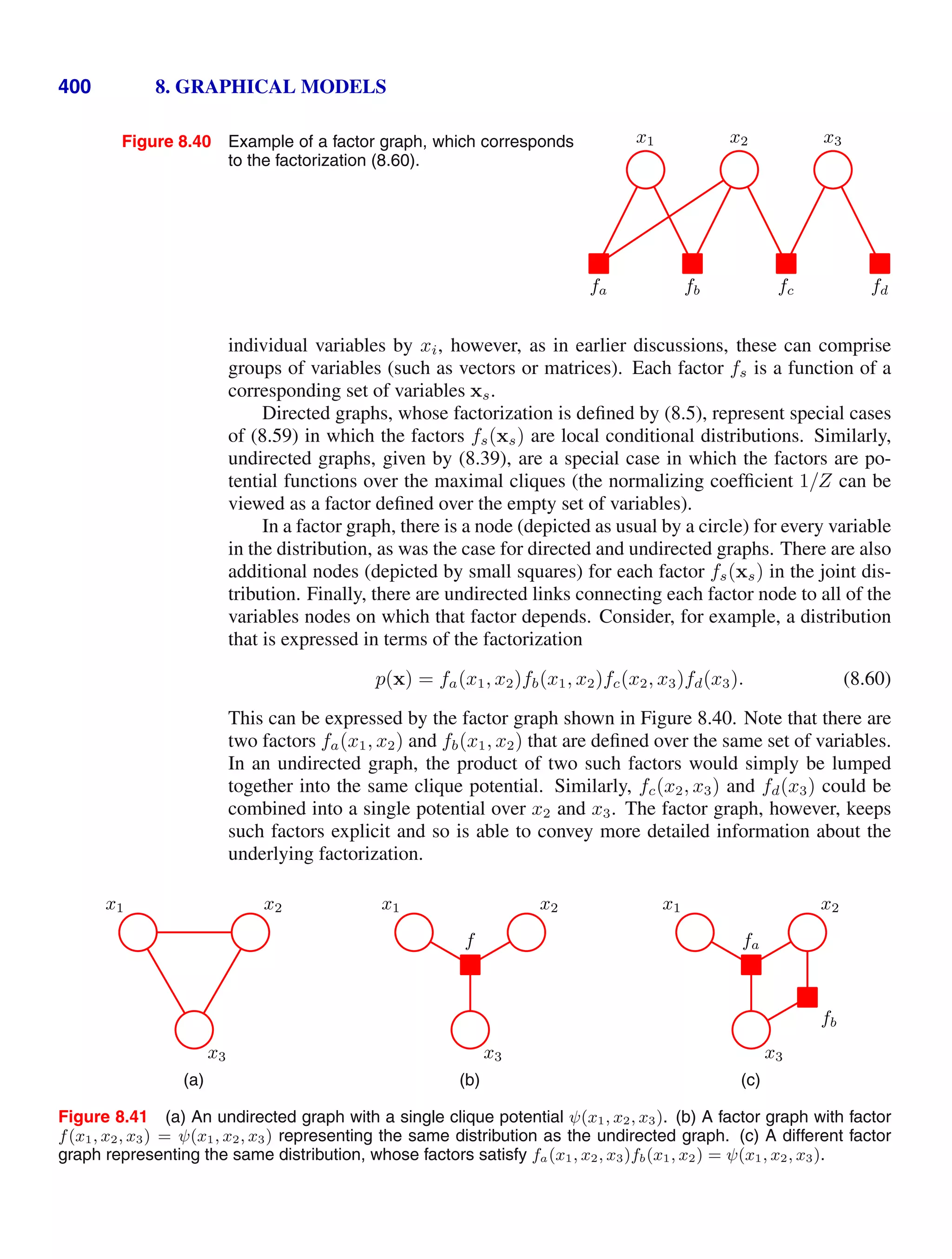
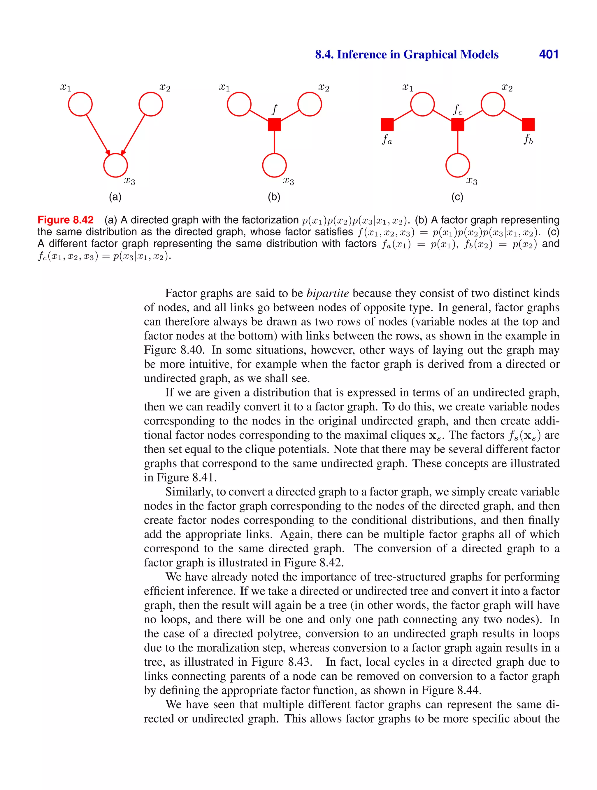
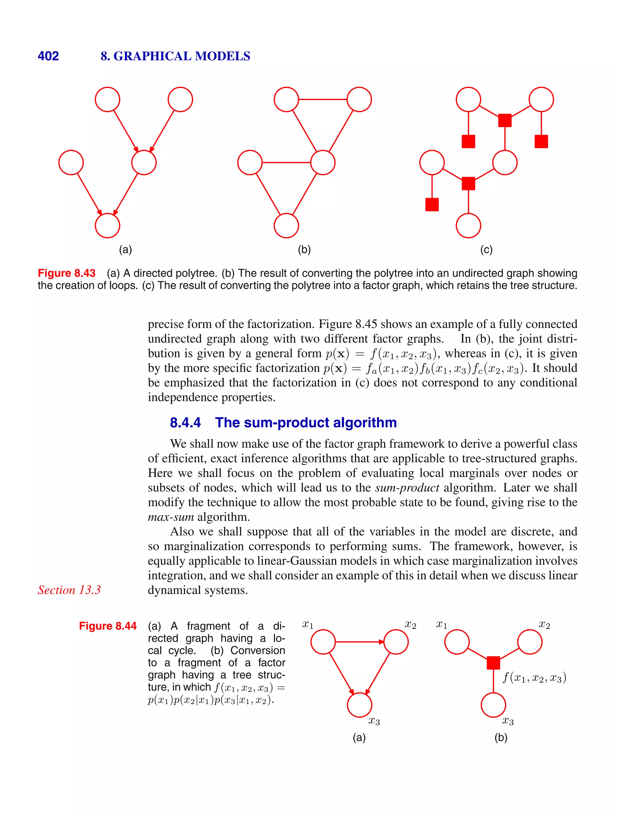
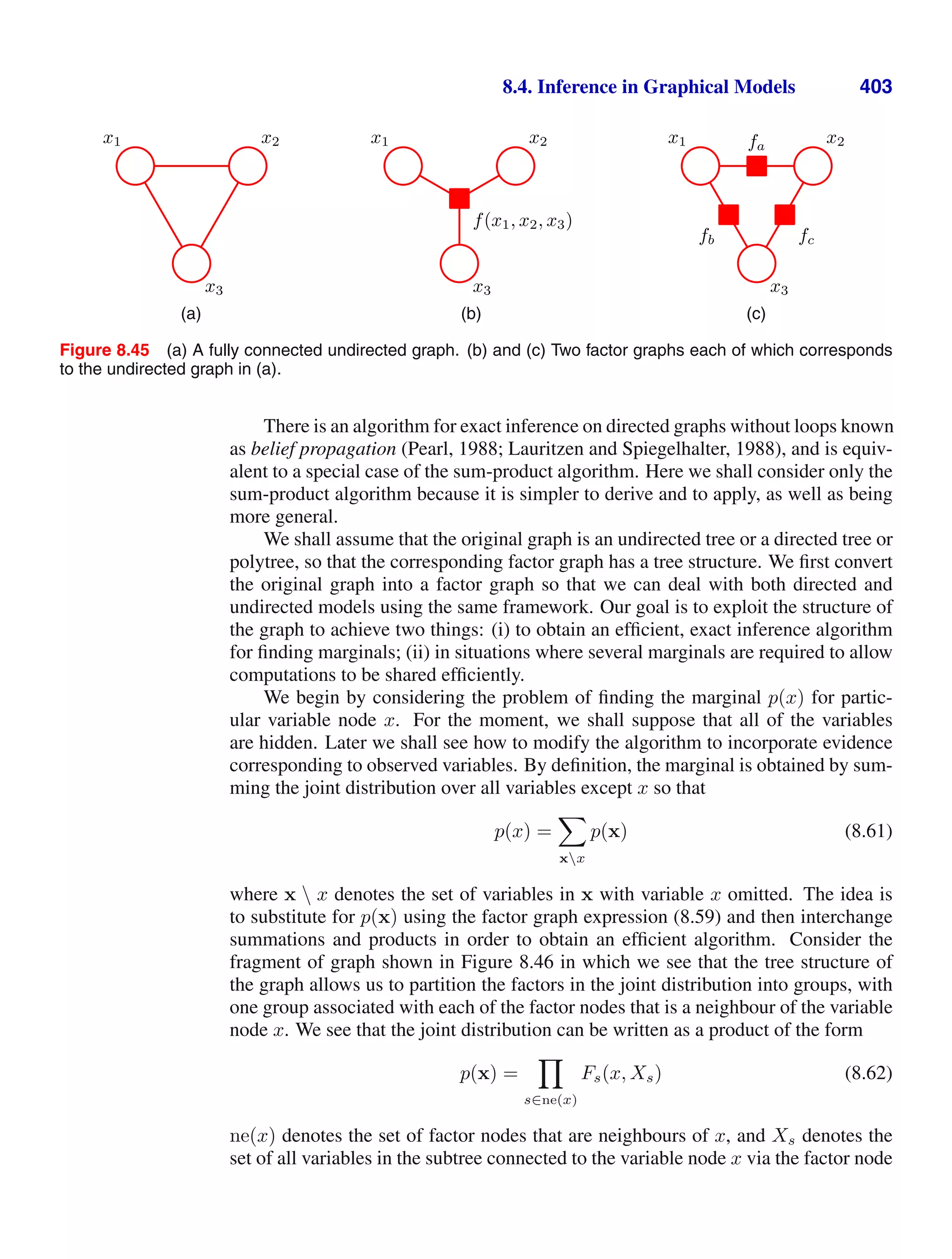
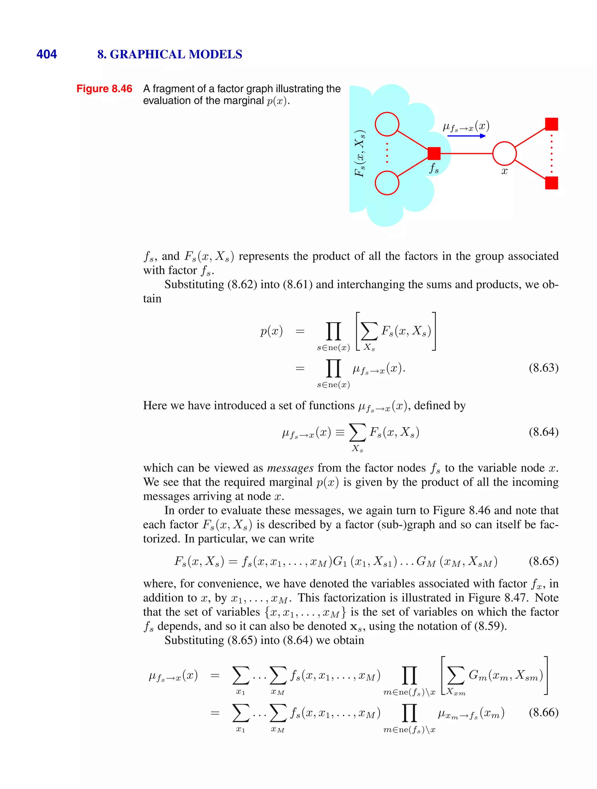
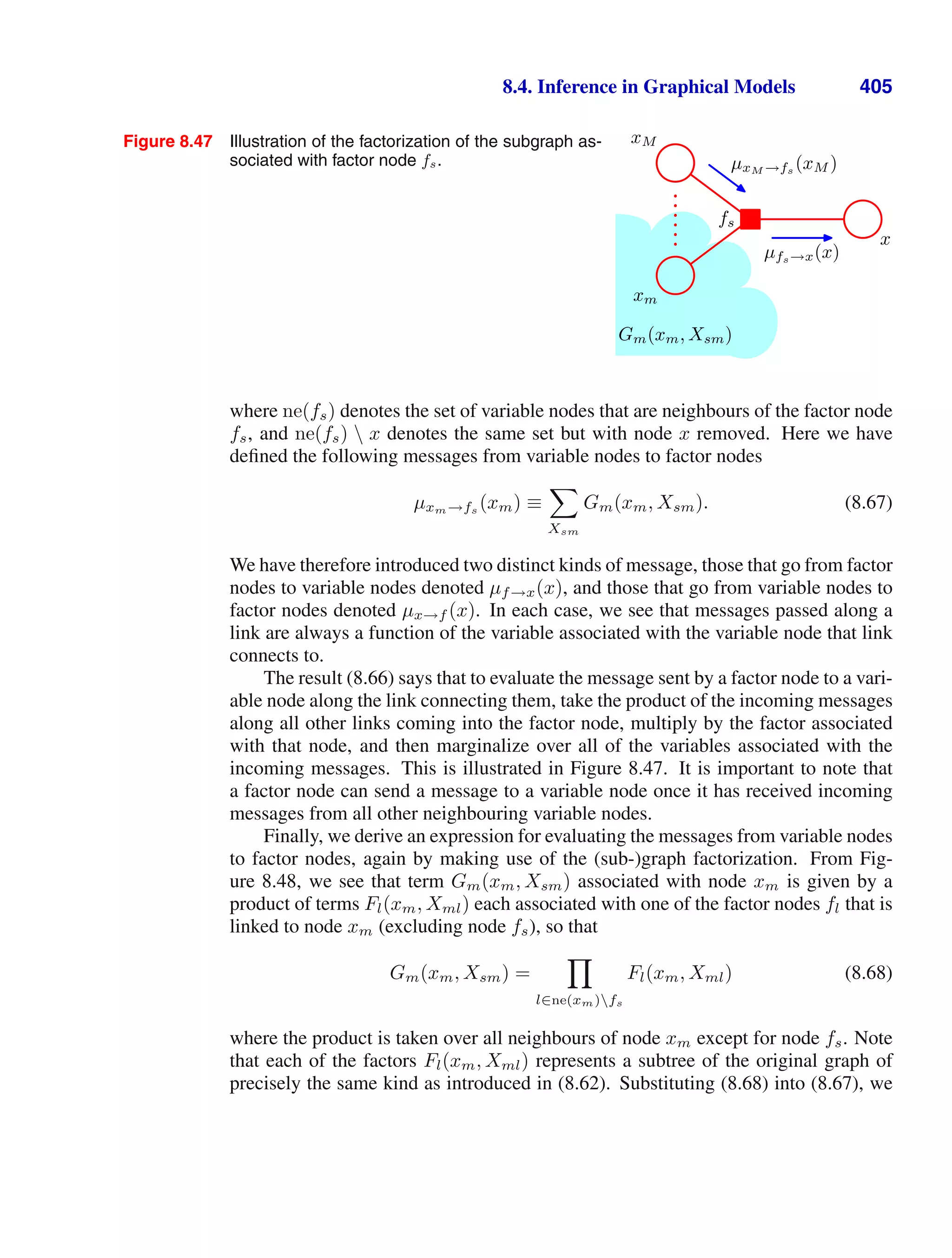
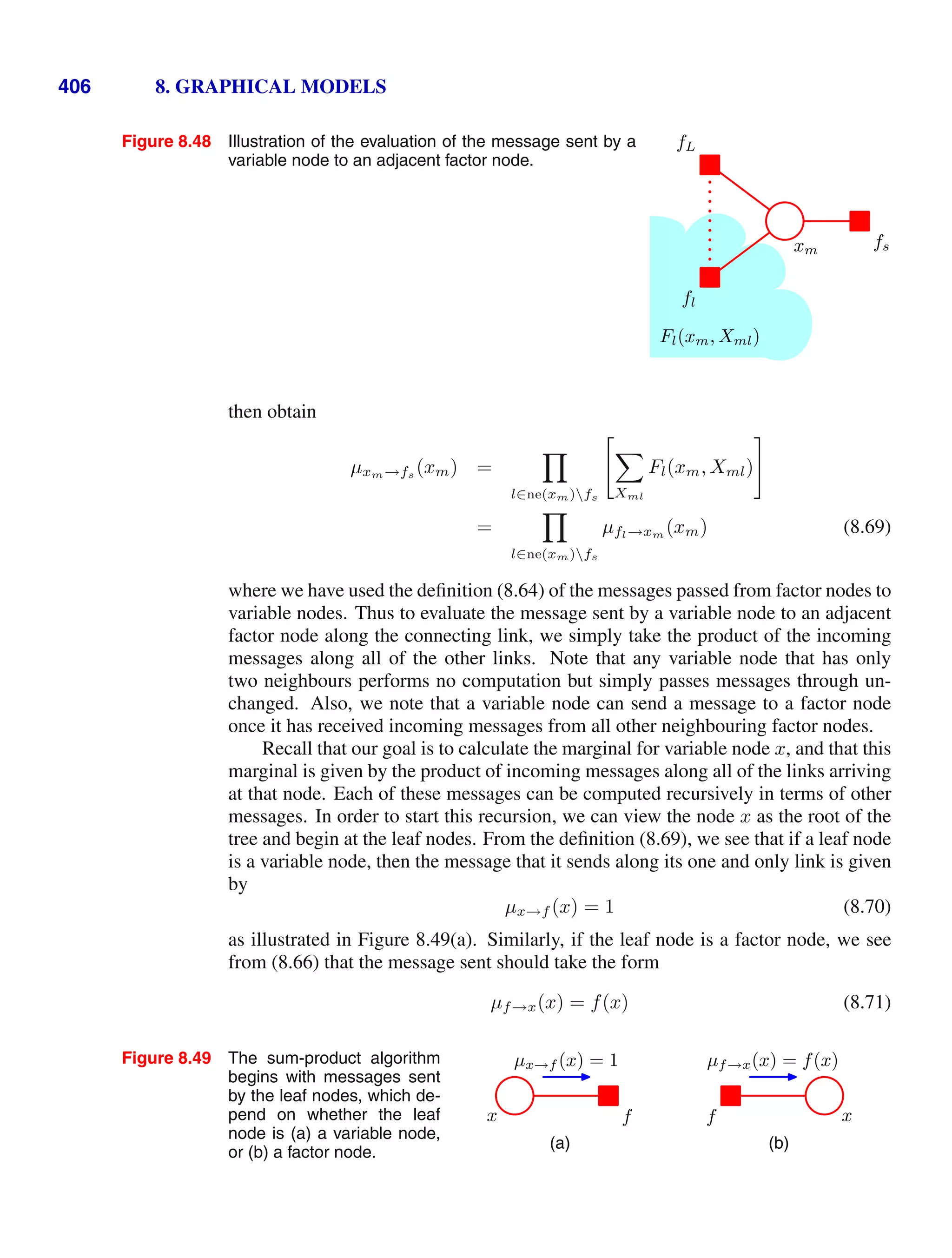
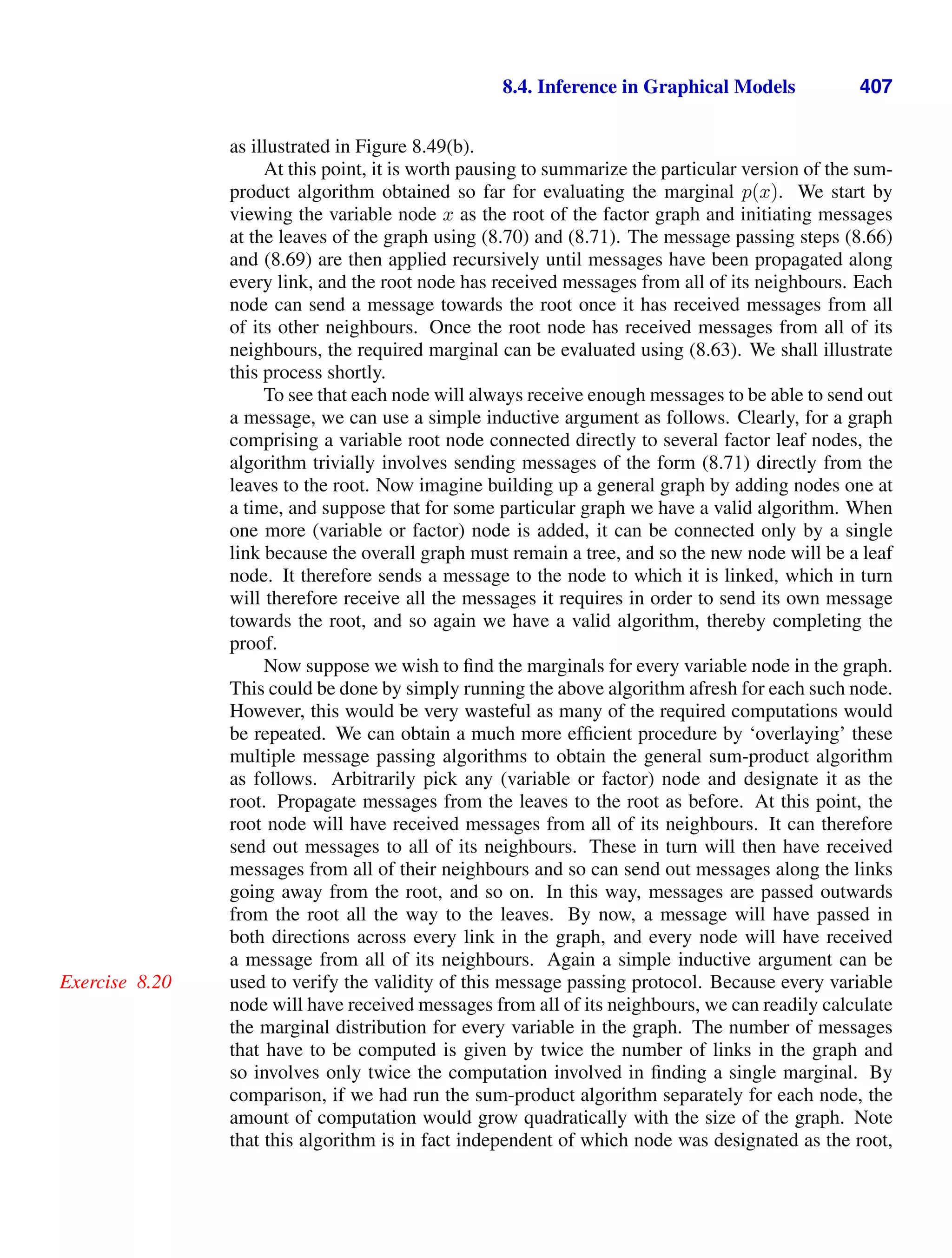
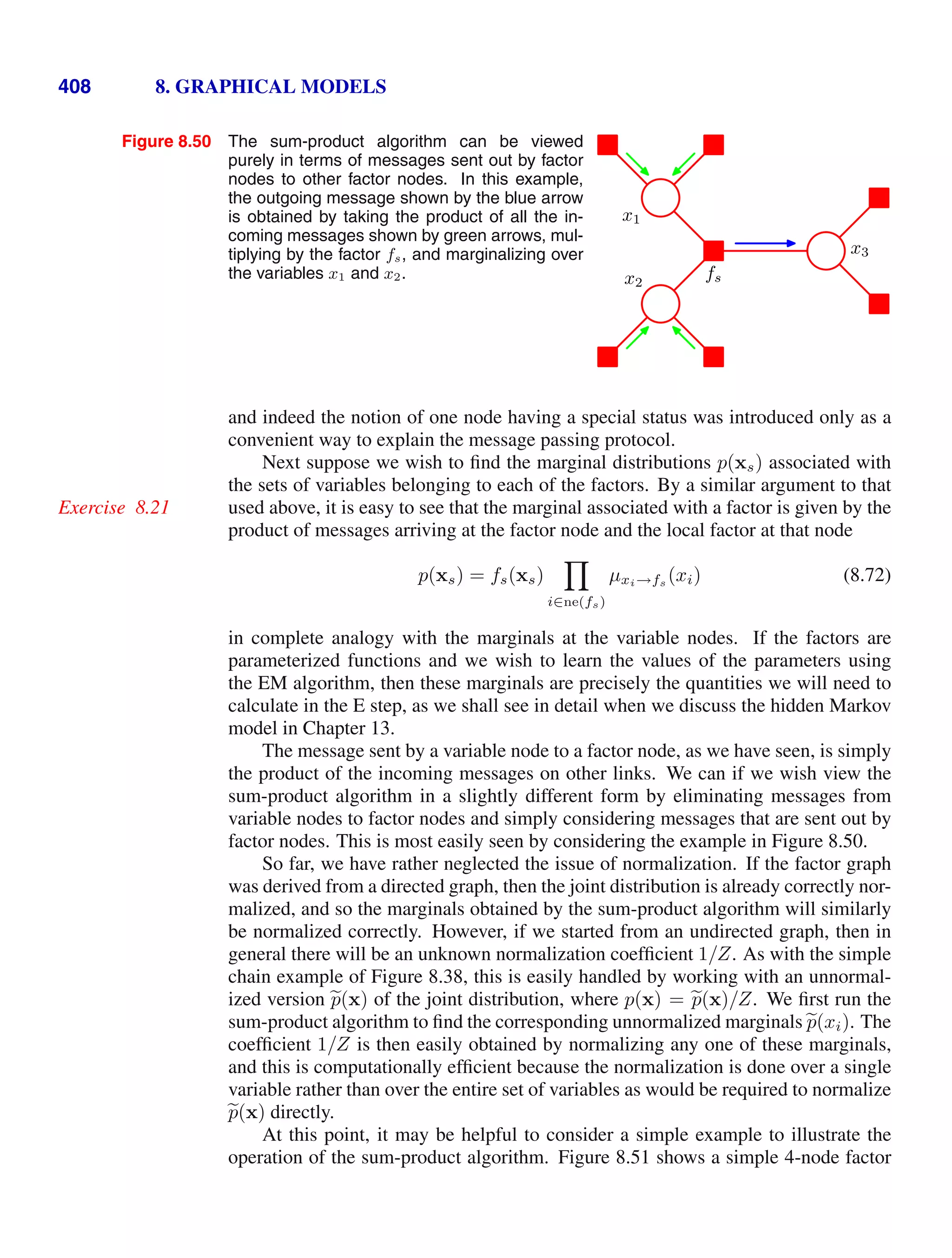
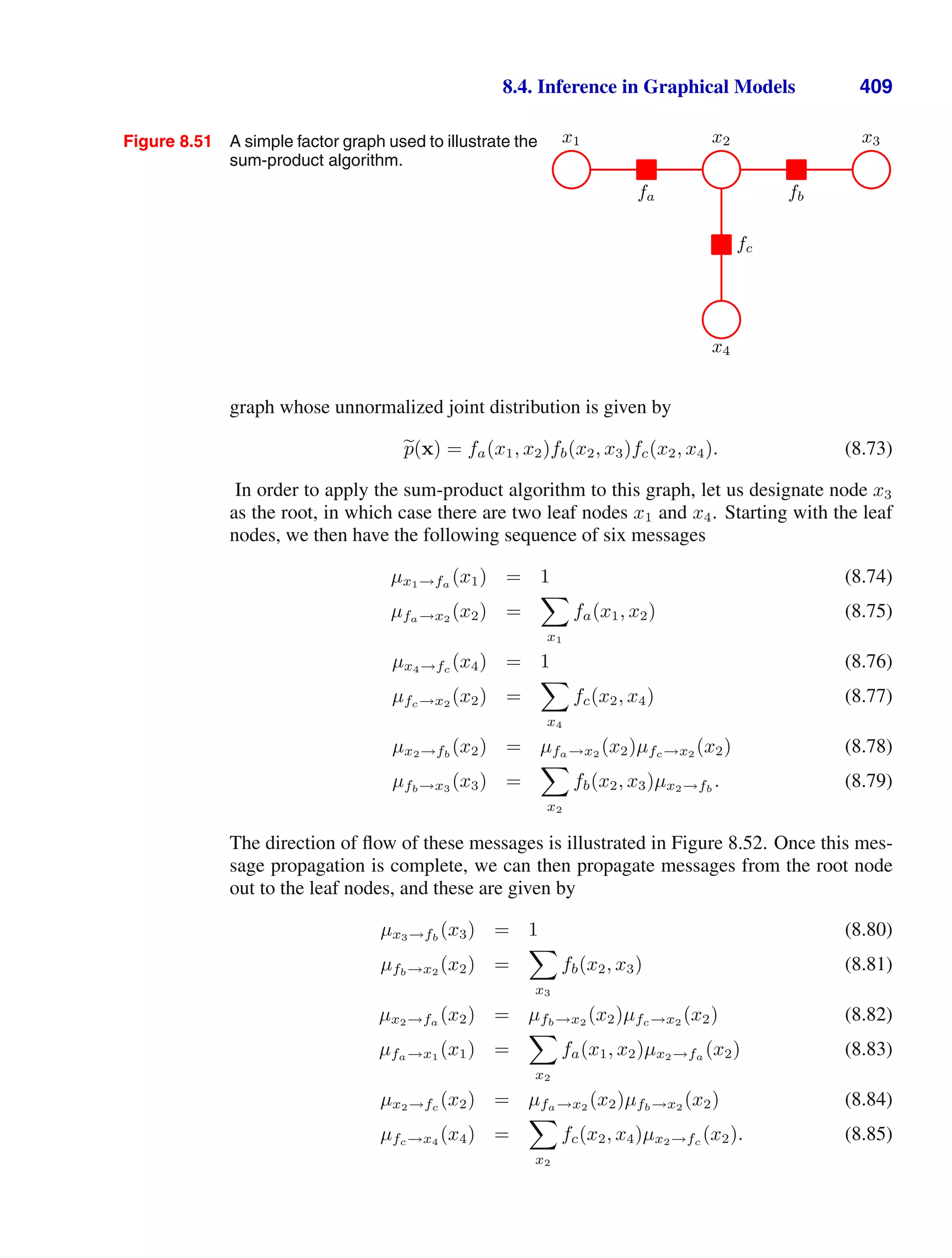
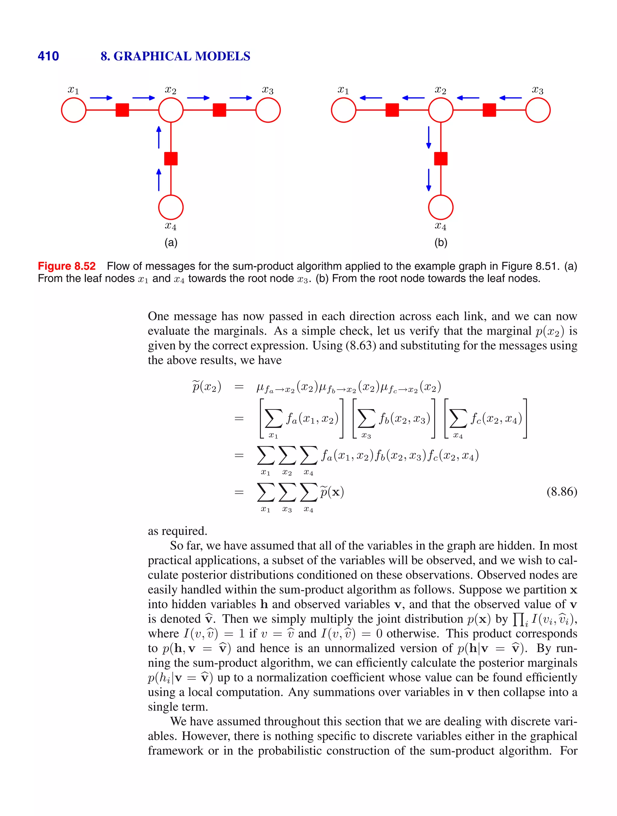
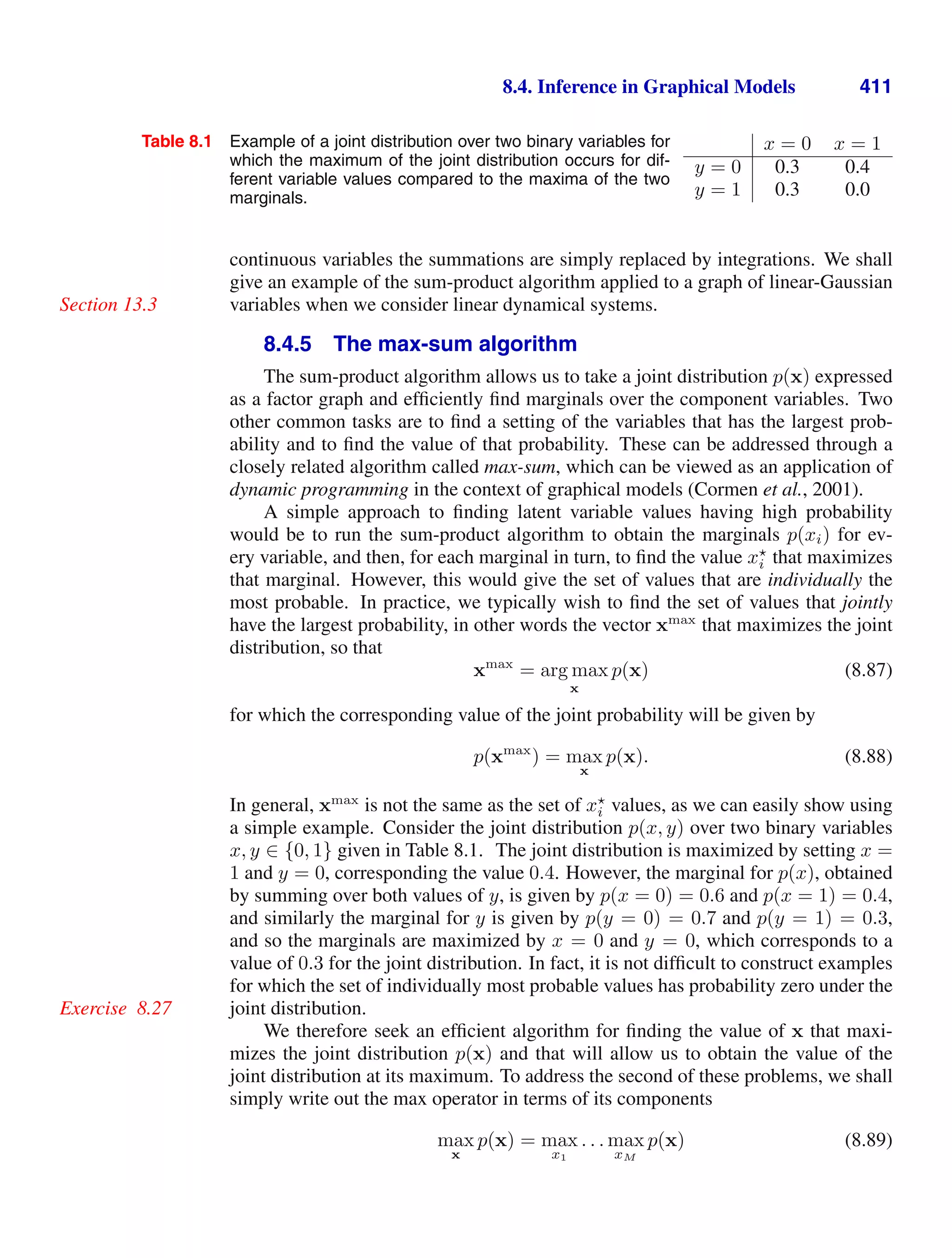
![412 8. GRAPHICAL MODELS
where M is the total number of variables, and then substitute for p(x) using its
expansion in terms of a product of factors. In deriving the sum-product algorithm,
we made use of the distributive law (8.53) for multiplication. Here we make use of
the analogous law for the max operator
max(ab, ac) = a max(b, c) (8.90)
which holds if a 0 (as will always be the case for the factors in a graphical model).
This allows us to exchange products with maximizations.
Consider first the simple example of a chain of nodes described by (8.49). The
evaluation of the probability maximum can be written as
max
x
p(x) =
1
Z
max
x1
· · · max
xN
[ψ1,2(x1, x2) · · · ψN−1,N (xN−1, xN )]
=
1
Z
max
x1
ψ1,2(x1, x2)
· · · max
xN
ψN−1,N (xN−1, xN )
.
As with the calculation of marginals, we see that exchanging the max and product
operators results in a much more efficient computation, and one that is easily inter-
preted in terms of messages passed from node xN backwards along the chain to node
x1.
We can readily generalize this result to arbitrary tree-structured factor graphs
by substituting the expression (8.59) for the factor graph expansion into (8.89) and
again exchanging maximizations with products. The structure of this calculation is
identical to that of the sum-product algorithm, and so we can simply translate those
results into the present context. In particular, suppose that we designate a particular
variable node as the ‘root’ of the graph. Then we start a set of messages propagating
inwards from the leaves of the tree towards the root, with each node sending its
message towards the root once it has received all incoming messages from its other
neighbours. The final maximization is performed over the product of all messages
arriving at the root node, and gives the maximum value for p(x). This could be called
the max-product algorithm and is identical to the sum-product algorithm except that
summations are replaced by maximizations. Note that at this stage, messages have
been sent from leaves to the root, but not in the other direction.
In practice, products of many small probabilities can lead to numerical under-
flow problems, and so it is convenient to work with the logarithm of the joint distri-
bution. The logarithm is a monotonic function, so that if a b then ln a ln b, and
hence the max operator and the logarithm function can be interchanged, so that
ln
max
x
p(x)
= max
x
ln p(x). (8.91)
The distributive property is preserved because
max(a + b, a + c) = a + max(b, c). (8.92)
Thus taking the logarithm simply has the effect of replacing the products in the
max-product algorithm with sums, and so we obtain the max-sum algorithm. From](https://image.slidesharecdn.com/bishop-patternrecognitionandmachinelearning-230316082240-9af1cdaa/75/Bishop-Pattern-Recognition-and-Machine-Learning-pdf-428-2048.jpg)
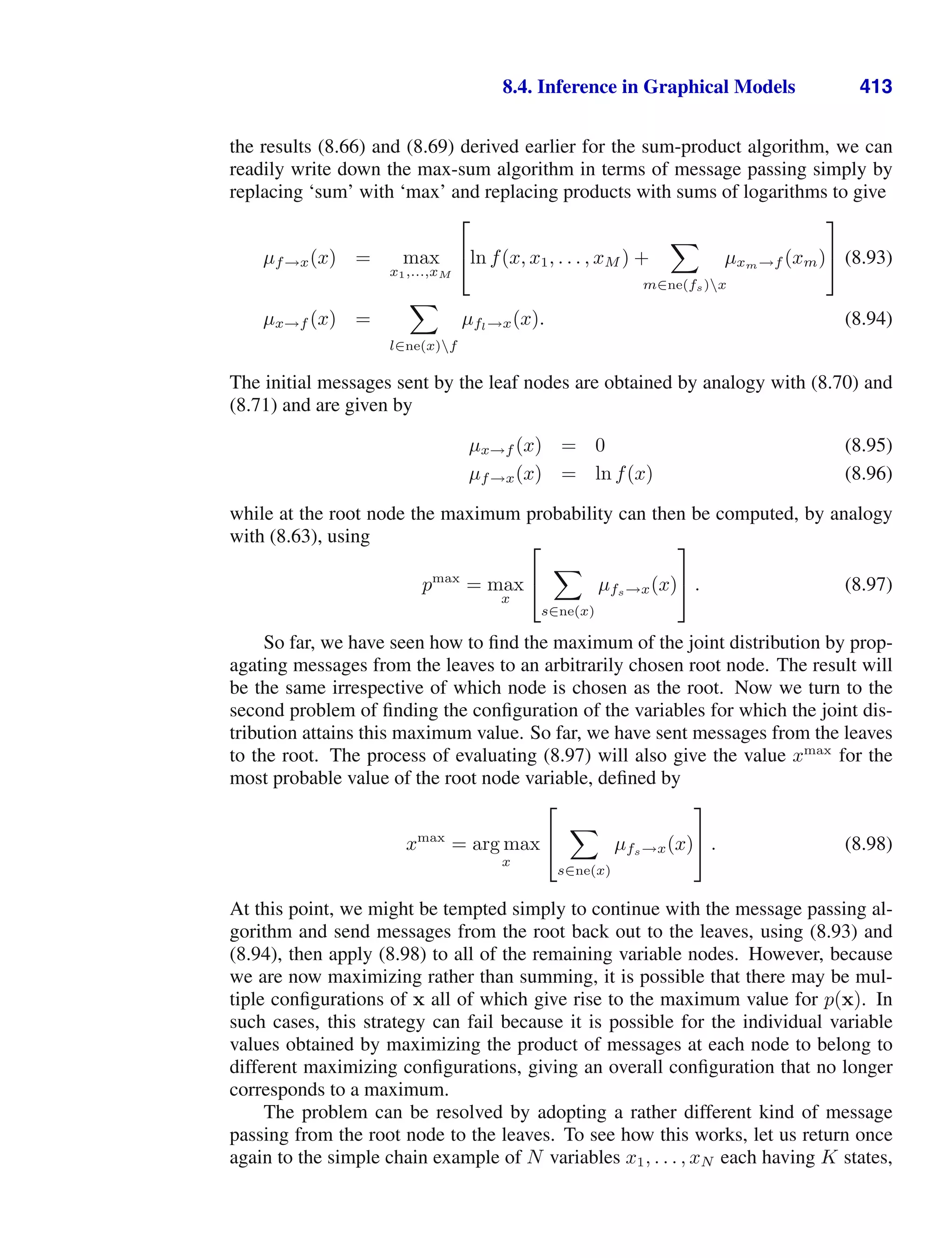
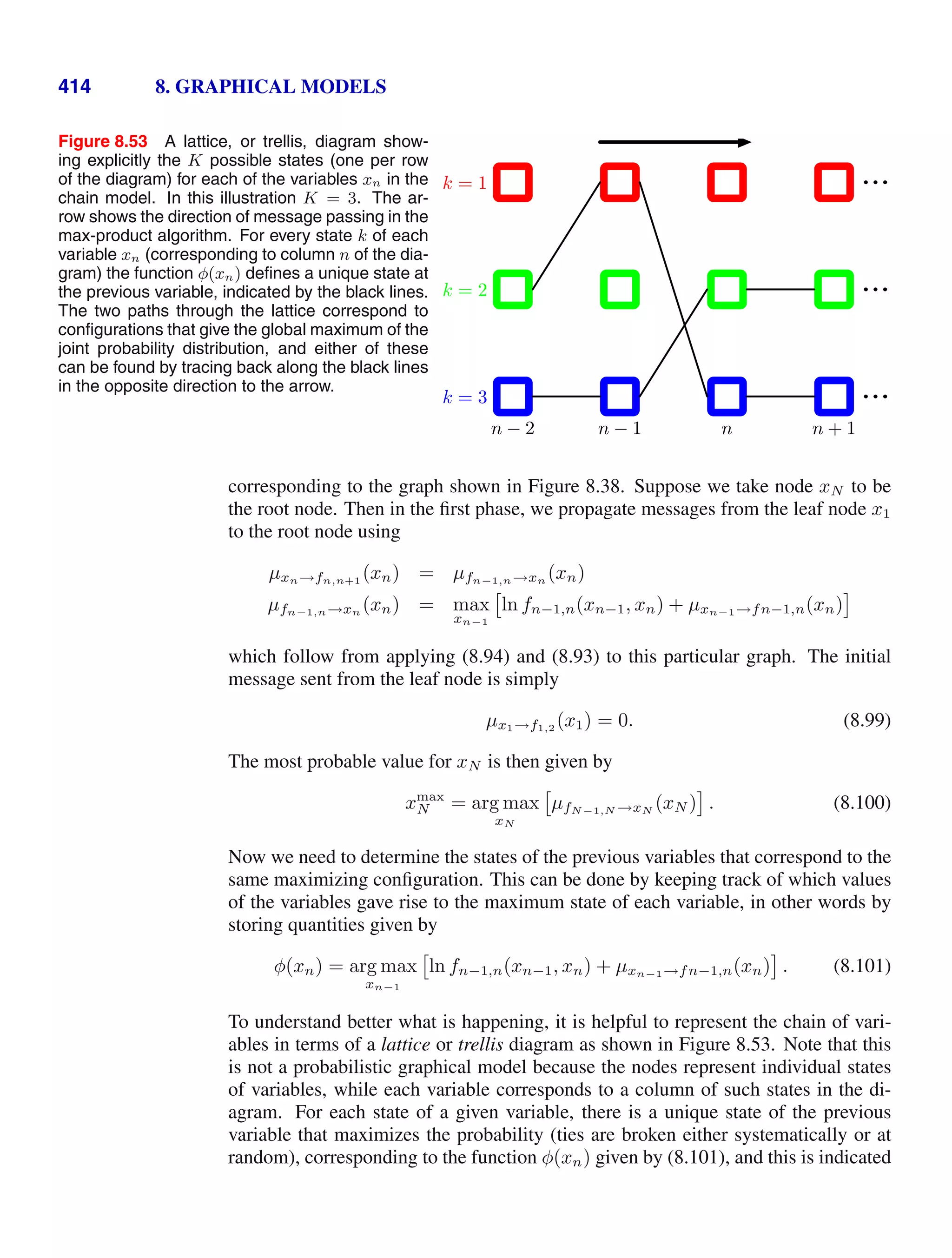

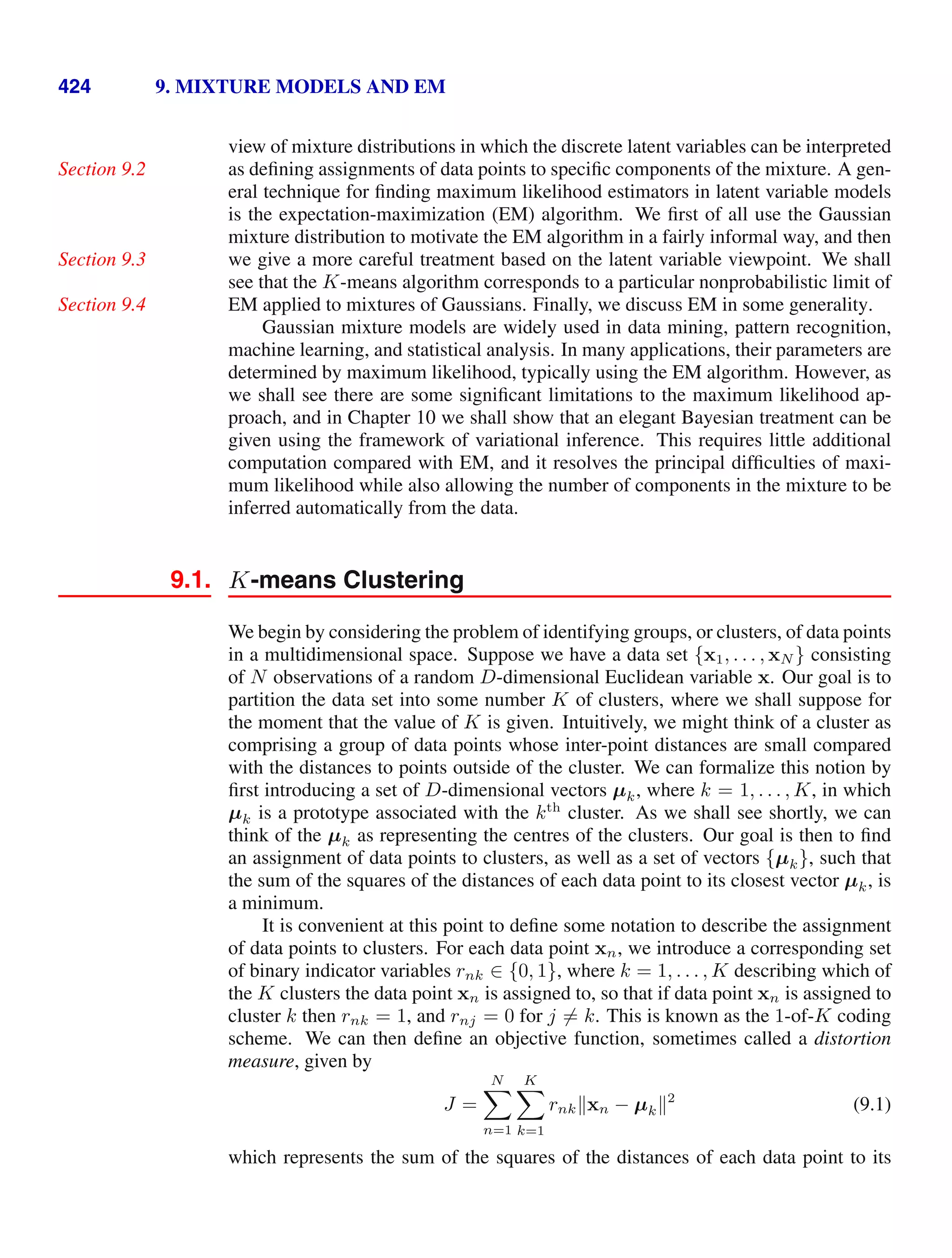
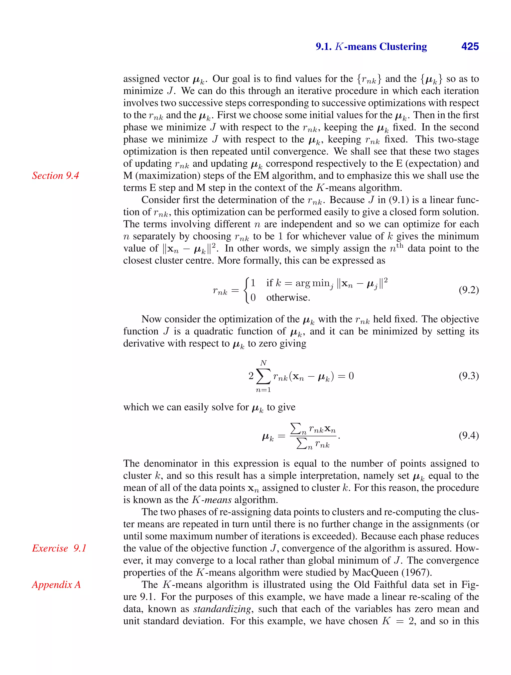
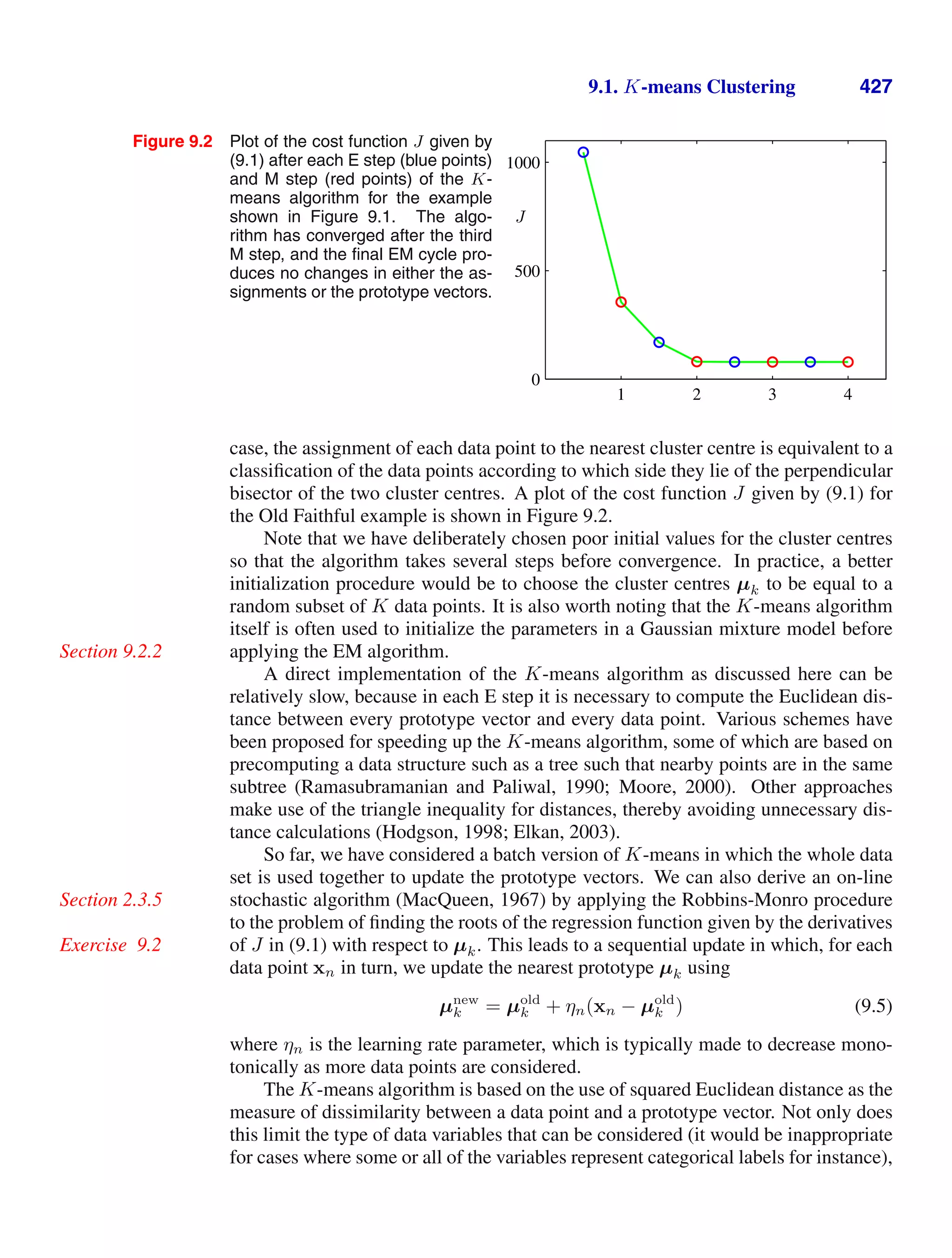
![428 9. MIXTURE MODELS AND EM
but it can also make the determination of the cluster means nonrobust to outliers. We
Section 2.3.7
can generalize the K-means algorithm by introducing a more general dissimilarity
measure V(x, x
) between two vectors x and x
and then minimizing the following
distortion measure
J =
N
n=1
K
k=1
rnkV(xn, µk) (9.6)
which gives the K-medoids algorithm. The E step again involves, for given cluster
prototypes µk, assigning each data point to the cluster for which the dissimilarity to
the corresponding prototype is smallest. The computational cost of this is O(KN),
as is the case for the standard K-means algorithm. For a general choice of dissimi-
larity measure, the M step is potentially more complex than for K-means, and so it
is common to restrict each cluster prototype to be equal to one of the data vectors as-
signed to that cluster, as this allows the algorithm to be implemented for any choice
of dissimilarity measure V(·, ·) so long as it can be readily evaluated. Thus the M
step involves, for each cluster k, a discrete search over the Nk points assigned to that
cluster, which requires O(N2
k ) evaluations of V(·, ·).
One notable feature of the K-means algorithm is that at each iteration, every
data point is assigned uniquely to one, and only one, of the clusters. Whereas some
data points will be much closer to a particular centre µk than to any other centre,
there may be other data points that lie roughly midway between cluster centres. In
the latter case, it is not clear that the hard assignment to the nearest cluster is the
most appropriate. We shall see in the next section that by adopting a probabilistic
approach, we obtain ‘soft’ assignments of data points to clusters in a way that reflects
the level of uncertainty over the most appropriate assignment. This probabilistic
formulation brings with it numerous benefits.
9.1.1 Image segmentation and compression
As an illustration of the application of the K-means algorithm, we consider
the related problems of image segmentation and image compression. The goal of
segmentation is to partition an image into regions each of which has a reasonably
homogeneous visual appearance or which corresponds to objects or parts of objects
(Forsyth and Ponce, 2003). Each pixel in an image is a point in a 3-dimensional space
comprising the intensities of the red, blue, and green channels, and our segmentation
algorithm simply treats each pixel in the image as a separate data point. Note that
strictly this space is not Euclidean because the channel intensities are bounded by
the interval [0, 1]. Nevertheless, we can apply the K-means algorithm without diffi-
culty. We illustrate the result of running K-means to convergence, for any particular
value of K, by re-drawing the image replacing each pixel vector with the {R, G, B}
intensity triplet given by the centre µk to which that pixel has been assigned. Results
for various values of K are shown in Figure 9.3. We see that for a given value of K,
the algorithm is representing the image using a palette of only K colours. It should
be emphasized that this use of K-means is not a particularly sophisticated approach
to image segmentation, not least because it takes no account of the spatial proximity
of different pixels. The image segmentation problem is in general extremely difficult](https://image.slidesharecdn.com/bishop-patternrecognitionandmachinelearning-230316082240-9af1cdaa/75/Bishop-Pattern-Recognition-and-Machine-Learning-pdf-444-2048.jpg)