Downloaded 114 times
![Quality score encoding
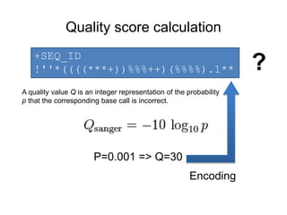
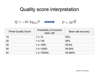
1. A quality score is typically: [0, 40]
http://ascii-table.com/img/ascii-table.gif
Not efficient space use
2. An ascii table contains 128 symbols, incl.
quality score range
3. Formula: score + offset => index
Two variants:
• offset=64(Illumina 1.0-before 1.8)
• offset=33(Sanger, Illumina 1.8+).
(33): !"#$%&'()*+,-./0123456789:;<=>?@ABCDEFGHI
(64): @ABCDEFGHIJKLMNOPQRSTUVWXYZ[]^_`abcdefgh](https://image.slidesharecdn.com/bioinfoformatvisualizationv2-140903095702-phpapp01/85/Bioinfo-ngs-data-format-visualization-v2-13-320.jpg)

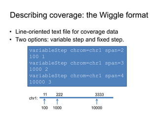

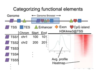
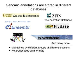
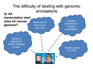
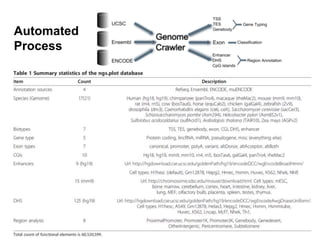
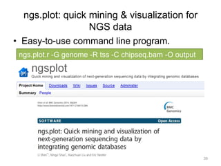
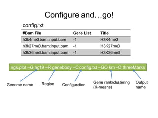


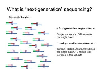
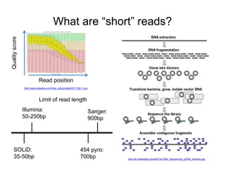
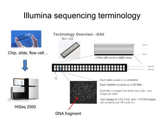
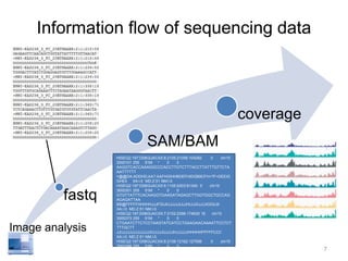
The document discusses data formats and visualization techniques in next-generation sequencing (NGS) analysis, detailing the advancements from first-generation sequencing methods to massively parallel NGS. It covers various sequencing technologies, file formats such as FASTQ and SAM/BAM, quality scoring systems, and the importance of alignment and coverage in genomic analysis. Additionally, it introduces tools for data processing, visualization, and accessing genomic annotation databases.


![제 23회 보아즈(BOAZ) 빅데이터 컨퍼런스 - [MBOAX] : ABSA를 활용한 소비자 반응 분석 기반 운영 효율화 대시보드 설계](https://cdn.slidesharecdn.com/ss_thumbnails/3-1boaz23rdconferencemboax-260203102709-9d519923-thumbnail.jpg?width=640&height=640&fit=bounds)


