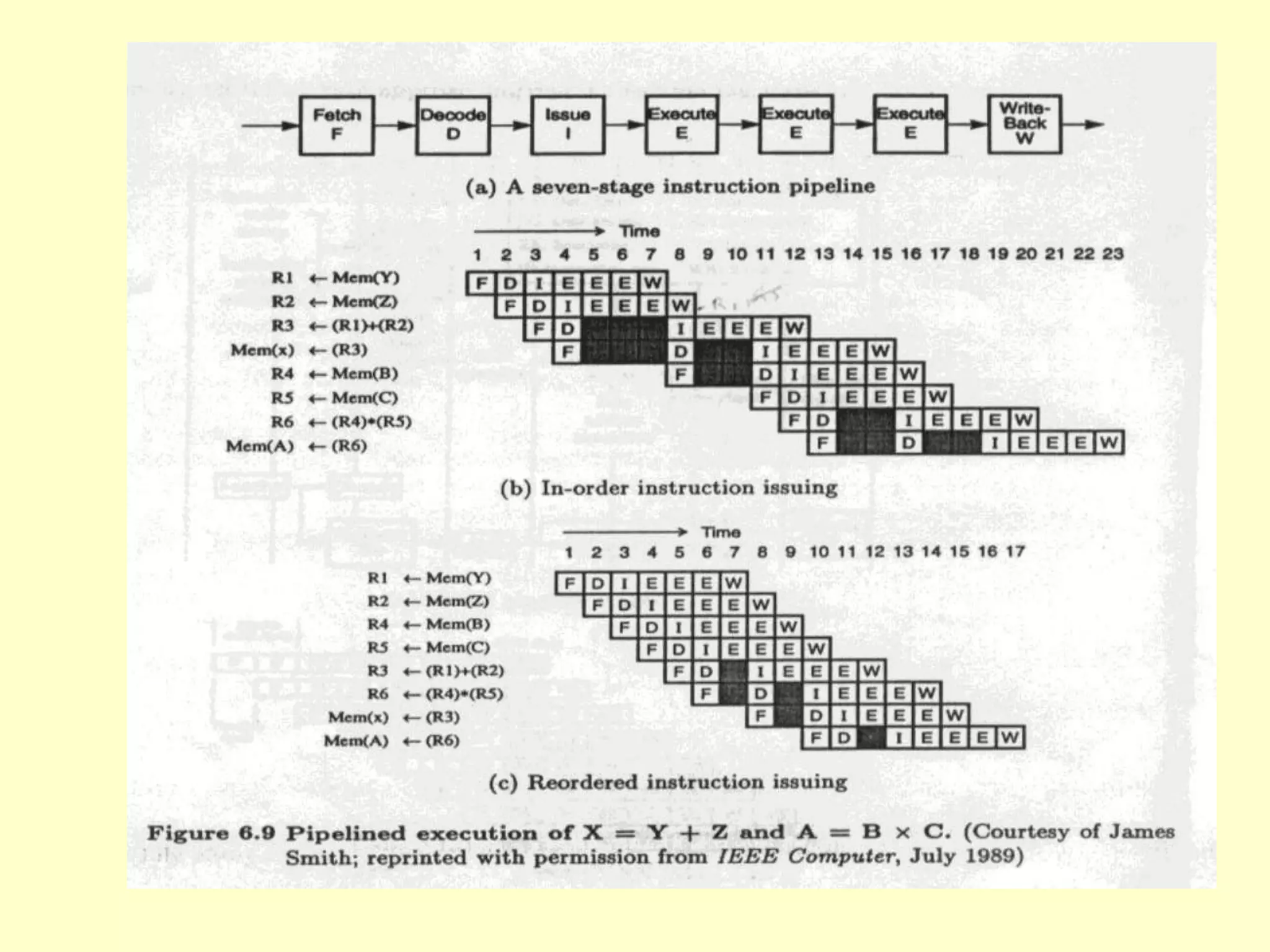
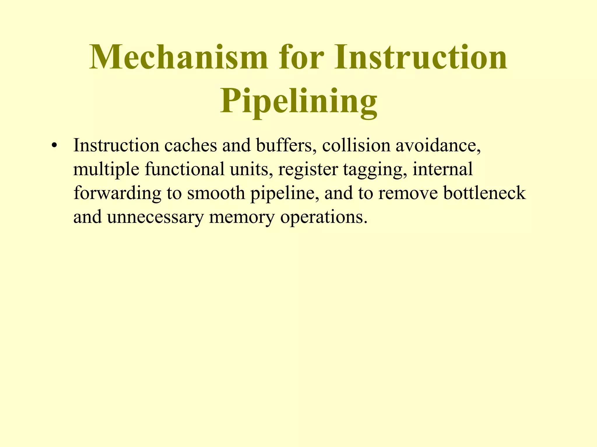
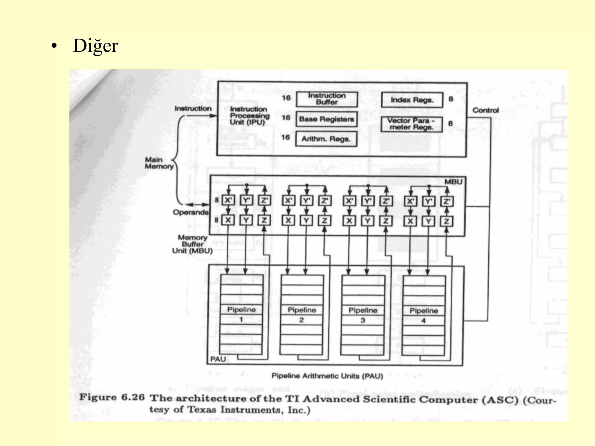
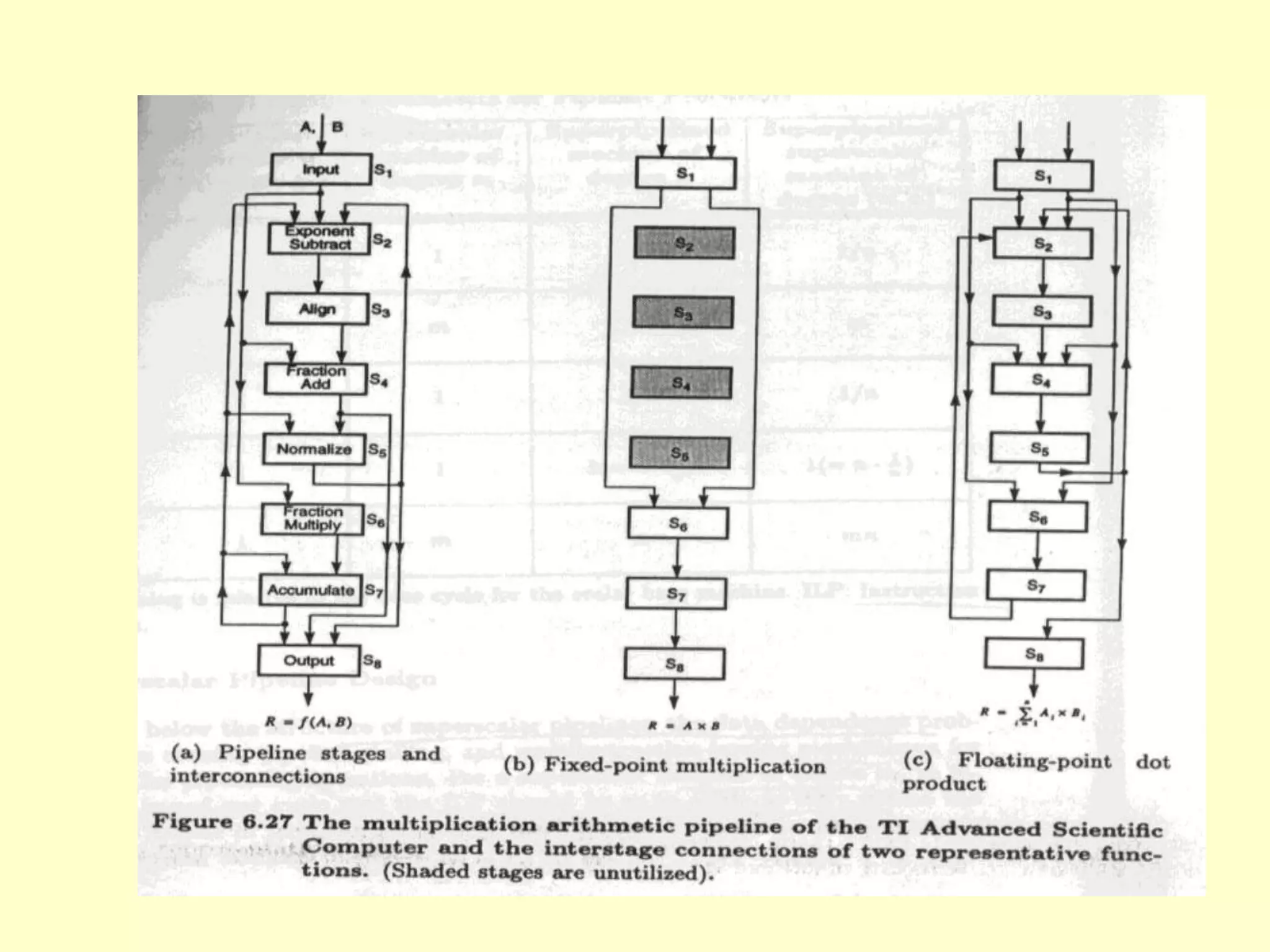
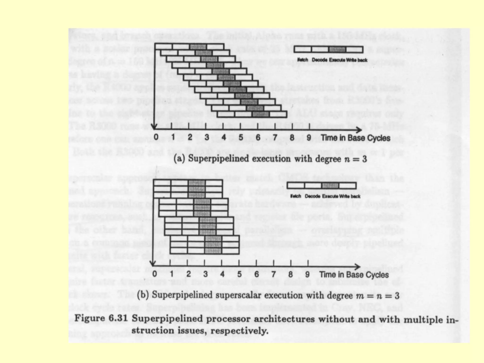
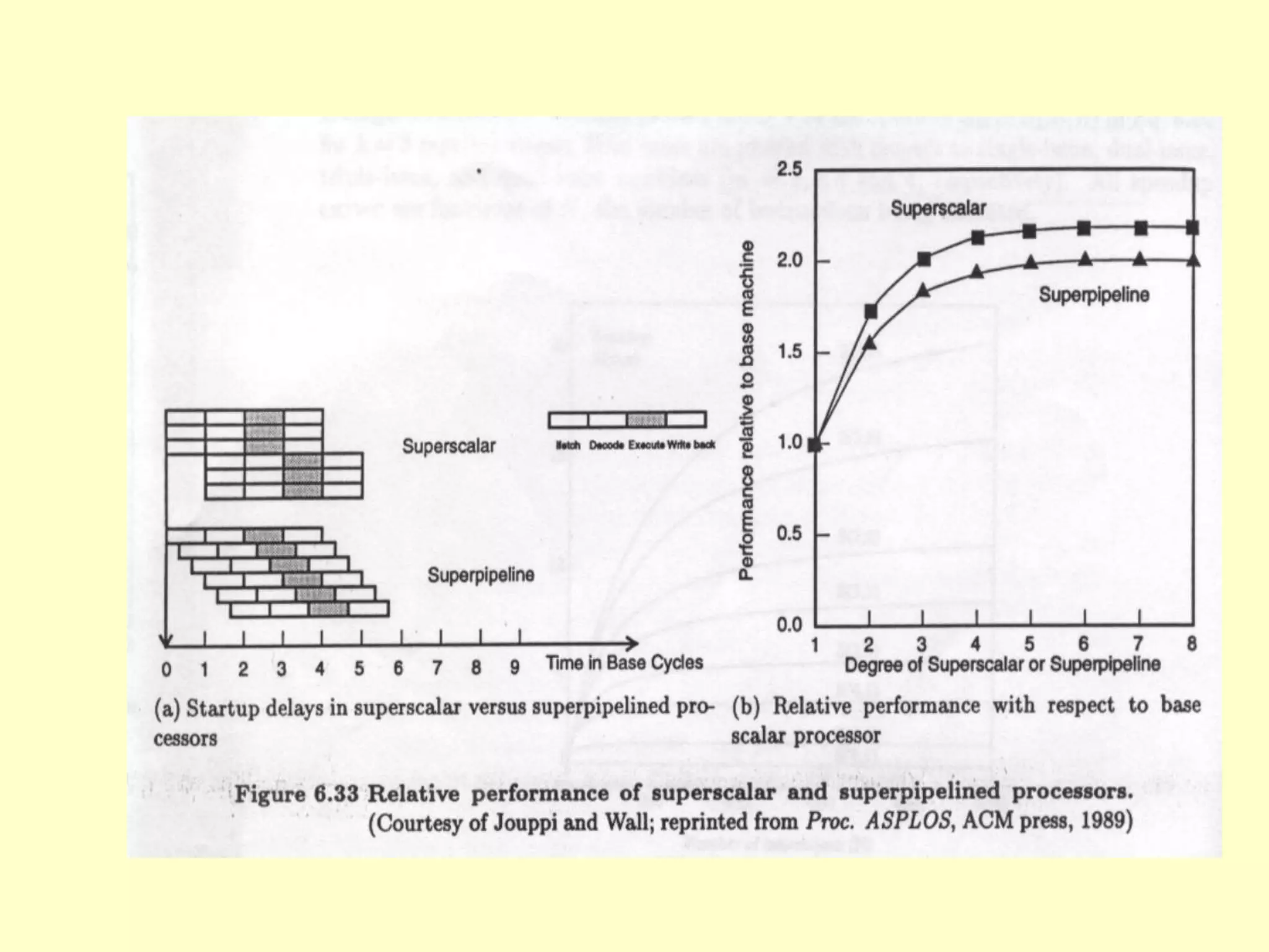
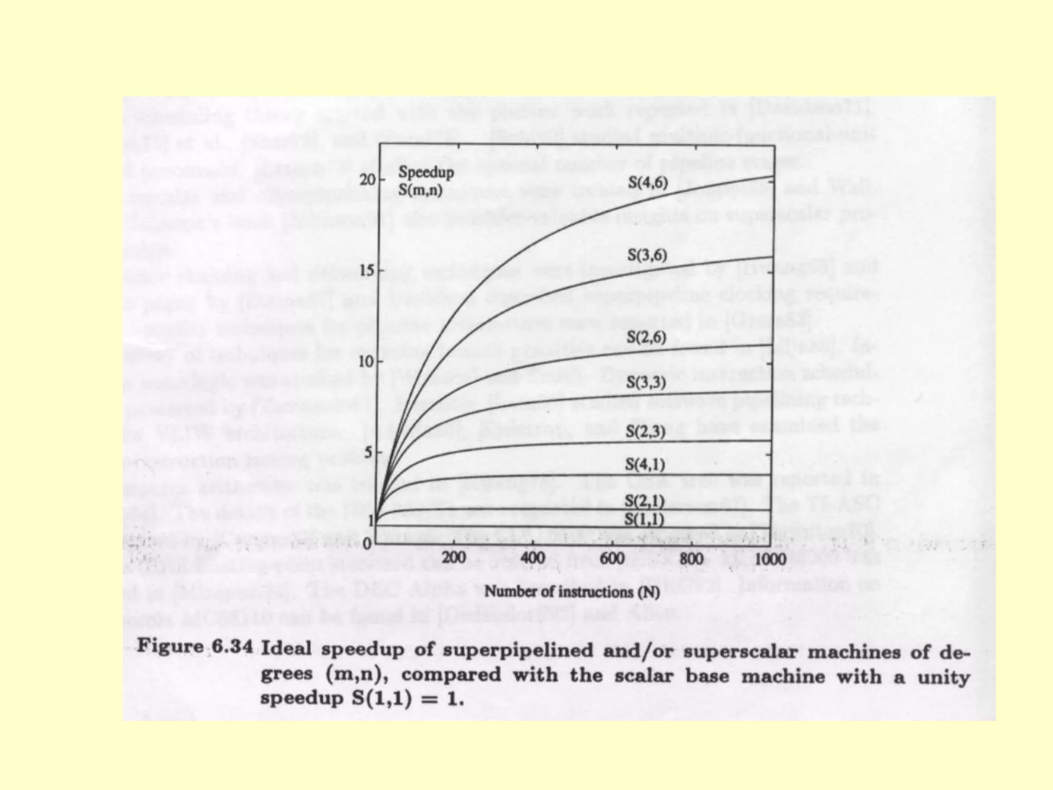
Chapter 7
Superscalar and
Superpipeline processors
Chapter7
Superscalar and Superpipeline Processors
• 7.1 MISD; Pipelining
• 7.2 Pipelining and Super Scalar
Techniques.
• 7.3 Linear Pipeline Processors; Asynchronous and
synchronous Models, Asynchronous Model,
Synchrones Model, Clocking and Timing Control,
Clock Cycle and throughput, Speedup Efficiency and
Optimal Number of stages
• 7.4 Nonlinear Pipelines; Reservation and latency analysis,
Reservation table, Latency Analysis, Collision Free
scheduling and Collision vector
• 7.5 Instruction Pipeline Design; Instruction Execution
Phase, Pre-fetching buffers, Loop buffers
• 7.6 Arithmetic pipelines
• 7.7 Superscalar and Superpipeline design; Pipeline
design parameters, Superscalar pipeline design, Super
scalar performance, Superpipeline design and
Superpipelined superscalar design
• 7.8 Super-symmetry and design Tradeoffs
7. 1 MISD: Pipelining
• MISD computer may consist of several instruction units
supplying similar number of processors, but these
processors all still obtain their data from single logical
source.
• This concept similar to pipelining architecture consists of
number of processors.
• Stream of data passed from one processor to the next.
• Each processor possibly performing different operations.
• Only applicable to specific task. (For example program
loops)
• There are instruction interdependence
• List of instruction must be coordinate with size of pipeline.
7.2 Pipelining and Super Scalar
Techniques.
• Advanced pipelining and super scalar processor
developments.
– A. Conventional linear pipelines analysis and
their performances
– B. Generalized pipeline model (including
nonlinear inter-stages connections)
– C. Collision-free scheduling techniques to
perform dynamic functions.
• Specific techniques for instruction, arithmetic,
and memory access pipelines.
• Instruction perfecting Internal data forwarding, software
interlocking, Hardware scoor-boarding, hazard avoidance,
branch handling, and instruction issuing.
• Static multifunctional arithmetic pipelines.
• Superpipelining and superscalar design techniques.
7.3 Linear Pipeline Processors
• Is cascade processing stage which linearly connected .
• Data flowing from one end to other end.
• Instruction execution
• Arithmetic computation
• Memory access operation
Asynchronous and
synchronous Models
• Constructed with K stages; Si to Si+1 > i:1,2, .. k-1.
•
• Depending control of flow; Pipelines may be modeled in
two categories; asynchronous and synchronous.
Asynchronous Model
• Data flow controlled by handshaking; (fotokopi page 266
Fig 6.1)
• When stage ready to transmit it send ready signal
• Next stage receives the signal and sends acknowledge.
• Useful to design communication Channel.
• Wormhole routing
• Variable throughput and different amounts of delay in
different stages.
Synchrones Model
• Fig 6.1.b page 266
• Clocked latches used to interface between stages
• Stages are combinational logic
• Delay are determined by clock period
• Pipeline utilization Fig 6.1.c diagonal stream line.
• K stage pipe needs k clock cycle for the result
• Successive task operations can be initiated at each clock
cycle
• One result emerges at each cycle
Clocking and Timing Control
• Clock cycle  of a pipeline determined below.
• i ;Circuitry delay, Si in Stage and
• d : time delay of a latch (fig 6.1b, page 266)
Clock Cycle and throughput
• m : maximum sage delay.
•
•  = maxi {i}1
k + d = m+d
•
• Pipeline frequency
•
• F = 1/
Speedup Efficiency
• K stages n tasks
• K+ (n-1)
• K cycle are needed to complete first task
• n-1 task require n-1 cycle, Total time
•
• Tk= [k +(n-1)] 
•
• : clock period,
•
• flow throughput is;
• T1= nk.
•
•
• Speedup factor is;
•
• Sk = T1/Tk=(nk)/(k+(n-1) =(nk)/(k+(n-1)
•
• Sk  k; (n  )
• Sk  1; (n  1)
Optimal Number of stages
• 2 < k < 15
• very few pipelines are designed to exceed 10 stages
•
• On the other hand coarse level for pipeline dages cen be
conducted at the processor level, called macro-pipelining.
•
• The optimal choice is pipeline stages should able to
maximize a performance /cost ratio.
• Fig. 6.2, page 269.
• T : nonpipelined execution time,
• k : number of sates,
• d : latch delay,
• p = t/k +d, program runs on k stage pipelines,
•
• f = 1/p = 1 /(t/k+d),
•
• total pipeline cost,
• c +kh,
• c :cost all logical stages,
• h :cost of latch
• A pipeline performance/cost ratio (PCR)
• PCR = f / (c+kh) = 1/((t/k+d)(c+kh))
• Ko= sqrt((t*c)/(d*h)); optimal stage number.
• Efficiency and throughput
•
• Ek = Sk/k = n /(k+(n-1))
• Ek  1; (n  )
• Ek  1/k; (n  1)
•
• Hk=n/[k+(n-1)]=nf/(k+(n-1)).
• Hk  Ek *f = Ek/=Sk/k; (n  )
• Hk  1/k; (n  1)
7.4 Nonlinear Pipelines
• Dynamic pipelines can be reconstructed to perform
variable functions at different times.
• Static pipelines performs fixed functions.
Reservation and latency
analysis
• Partitioning in a dynamic pipeline becomes quite involved;
(loops and stages are interconnected)
•
• (Fig 6.3.a, page 271).
• There are straight connections and feedbacks.
•
• These feedfowards and feedbacks makes the scheduling of
successive events in the pipeline nontrivial task.
Reservation table
• Static pipeline is trivial in the sense that data flows a
linear stream.
• The reservation table for dynamic pipeline becomes more
interesting because a nonlinear pattern is followed.
• Two representation table are give in fig 6.3. corresponding
X and Y functions.
• The number of columns are called the evaluation time.
• X requires 8 clock cycle and Y 6 clock cycle.
• Static pipeline uses same reservation table.
• Check marks correspond to a particular stage will be used
at a certain cycle. (multiple check marks in a row, which
means repeated usage of the stage indifferent cycle and in
column is parallel execution at multiple stages.
Latency Analysis
• Latency is the time units between two initiations of a
pipeline (for example k cycle).
• To use the same pipeline stage at the same time will cause
collision.
• A collision implies conflict between two initiations in th
pipeline.
• Same latency causes collision and some not.
• The latency causes collision is forbidden latency.
• Fig 6.4, page 272.
Collision Free scheduling
• Objectives.
• Shortest average latency between initiations without
collision.
• Use ; collision vector, state diagrams, single cycles greedy
cycles and minimal average latency.
Collision vector
• For fig. 6.3 Cx = (1010010) and Cy(1010)
•
• Cx için latency 7,5,4,an 2 forbidden and 6,3,1 permissible.
• Cy için latency 4, 2 forbidden and 3,1 permissible.
•
•
• Explain in the figure (fig 6.3 page 271).
• Diğer
7.5 Instruction Pipeline Design
• A stream of instructions can be executed by a pipeline in
an overlapped manner.
• CISC and RISC uses instruction pipeline.
• Instruction pre-fetching, data forwarding, hazard
avoidance, interlocking for resolving data dependencies,
dynamic instruction scheduling, and branch handling
techniques for improving pipelined processors
performance.
Instruction Execution Phase
• A typical execution consist of a sequence of operations,
including instruction fetch, decode, operand fetch, execute
and write-back phases.
• These phases are overlapped on a linear pipeline.
• Each phase require one or more clock cycle depending on
the architecture.
Pipeline instruction processing
• A typical instruction pipeline is depicted on (fig 6.9, page
281)
• F (Fetch stage): fetches instruction.
• D (decode stage ): decodes instruction and identitifies
resources are needed. (General registers, busses and
function units.
• I (issue stage): Reserves resources.
• E ( X-Execute stage) :
• W (write-back stages :
• X =Y+Z = and A= BxC (Explain on CISC and RISC and
explain on the figure (Şekil 6.9 sonuç var)
Mechanism for Instruction
Pipelining
• Instruction caches and buffers, collision avoidance,
multiple functional units, register tagging, internal
forwarding to smooth pipeline, and to remove bottleneck
and unnecessary memory operations.
• Diğer
Pre-fetching buffers
• Three (four) type of buffers; (fig 611, page 283)
• Prefetch buffers; used to shorten memory access time,
•
• Sequential buffers; Sequential instruction loaded in to a
pair of sequential buffers.
•
• Target buffers; Instruction from a branch target are loaded
into a pairs of target buffers for out of sequence pipelining.
Loop buffers;
• Holds sequential instruction contained in a small loop. U
loop boundaries recognized and unnecessary memory
accessed can be avoided.
Multiple functional units
• (Figure 6.12, page 284.) Tag unit keeps checking the tags
from all currently used registers or RSs
Internal data forwarding
• (Fig 6.13, page 285, açıkla)
•
• Store and forward;
•
• Load-load forwarding; eliminates second load operations.
•
• Store-store forward;
•
• (Figure 6.14, Internal data forwarding)
Hazard avoidance;
• Fig 6.15 page 287.
•
• R(I) n D(j)  For RAW hazard (Flow dependence)
• R(I) n R(j)  For WAW hazard (Antidependence)
• D(I) n R(j)  For WRAR hazard (ouptput dependence)
• D(I), R(I) domain I instruction
Dynamic scheduling
• Static scheduling is supported by an optimizing compiler
• Dynamic scheduling is achieved by Tomasulo’s register
tagging schema.
• Example on page 288.
• Tomasulo’s algorithm ; This schema resolves resource
conflicts as well as data dependencies using register
tagging to allocate and de-allocate source and destination
registers. An issued instruction whose operands are not
available.
• It waits until data dependencies have been resolved and its
operand become available.
• (Figure 6.16, page 290.)
Branch handling techniques
• Performance of pipeline processors is limited by the data
dependencies and branch instructions.
•
• Various instruction issuing logic and resource monitoring
schemas were described.
IEEE Floating-Point Standards
• Diğer
• Diğer
• Diğer
• Diğer
• Diğer
• Diğer
• Diğer
• Diğer
7.6 Arithmetic pipelines
• Pipelining techniques can be applied to speed up numerical
arithmetic computations (fixed point and floating point
operations).
•
• Sayfa 298 floating point sayı yapısı ve
• Sayfa 299 aritmetik işlemler.
•
• (Fig 6.27, page 6.27)
7.7 Superscalar and
Superpipeline design
• Architectural approache is used to improve performance of
machine.
• Based on sperscalar pipelining techniques andtecnology.
Pipeline design parameters
• The machine pipeline cycle is the base cycle
• Instruction Issue rate,
• Instruction Issue latency, and
• Simple operation latency.
•
• Table 6.1, page 310.
Superscalar pipeline design
• m-issue superscalar processor.
•
• Fig 6.28, page 311.
•
• Data dependencies;
• Pipeline stalling (proper scheduling may avoids pipeline
stalling) (fig 6.29, page 313)
• In-order issue (sıralı koşmal).
• Out-of-order Issue (sırasız koşma) (fig 6.30, page 314).
• Diğer
• Diğer
Super scalar performance
• T(m,1) k + (N-m)/m
•
• N : independent instruction
• m: pipelines simultaneous
• k : time required to run first m instruction.
•
• S(m,1) = m*(N+k-1)/(N+m*(k-1))
• N >> sonsuz ; S(m,1) >> m
Superpipeline design
• Processor degree n the cycle time is 1/n
• (fig 6.31, page 317)
•
• T(1,n)= k + (N-1)/n (base cycle),
•
• S(1,n)= n*(k+N-1)/(n*k+N-1)
•
• Superpipelined and superscalar design (in figure 6.31).
Superpipelined superscalar
design
• T(m,n) and S(m,n)
• (Fig 6.3.b, page 317)
• T(m,n) = k + (N-m)/(m*n)
• S(m,n) = (mn*(k+N-1)/(mnk+N-m)
• S(m,n) >> mn N >> sonsuza
• Dublicating hardware source such as execution units and
registers and ports,
• Emphasize temporal parallelism – overlapping multiple
operations on a common piece of hardware.
• Faster clock cycles for deeply pipelined execution units.
• Diğer
7.8 Super-symmetry and design
Tradeoffs
• (fig 6.33, page 320)
•
• Super pipelined machine has a longer startup delay and
lags behind the superscalar machine (lag :geriden geliyor).
• Branch create more damage on superpipelined machine.
•
• (fig 6.34, page 321)
BIL406-Chapter-7-Superscalar and Superpipeline  processors.ppt

BIL406-Chapter-7-Superscalar and Superpipeline processors.ppt

  • 1.
  • 2.
    Chapter7 Superscalar and SuperpipelineProcessors • 7.1 MISD; Pipelining • 7.2 Pipelining and Super Scalar Techniques. • 7.3 Linear Pipeline Processors; Asynchronous and synchronous Models, Asynchronous Model, Synchrones Model, Clocking and Timing Control, Clock Cycle and throughput, Speedup Efficiency and Optimal Number of stages • 7.4 Nonlinear Pipelines; Reservation and latency analysis, Reservation table, Latency Analysis, Collision Free scheduling and Collision vector • 7.5 Instruction Pipeline Design; Instruction Execution Phase, Pre-fetching buffers, Loop buffers
  • 3.
    • 7.6 Arithmeticpipelines • 7.7 Superscalar and Superpipeline design; Pipeline design parameters, Superscalar pipeline design, Super scalar performance, Superpipeline design and Superpipelined superscalar design • 7.8 Super-symmetry and design Tradeoffs
  • 4.
    7. 1 MISD:Pipelining • MISD computer may consist of several instruction units supplying similar number of processors, but these processors all still obtain their data from single logical source. • This concept similar to pipelining architecture consists of number of processors. • Stream of data passed from one processor to the next. • Each processor possibly performing different operations. • Only applicable to specific task. (For example program loops) • There are instruction interdependence • List of instruction must be coordinate with size of pipeline.
  • 5.
    7.2 Pipelining andSuper Scalar Techniques. • Advanced pipelining and super scalar processor developments. – A. Conventional linear pipelines analysis and their performances – B. Generalized pipeline model (including nonlinear inter-stages connections) – C. Collision-free scheduling techniques to perform dynamic functions. • Specific techniques for instruction, arithmetic, and memory access pipelines.
  • 6.
    • Instruction perfectingInternal data forwarding, software interlocking, Hardware scoor-boarding, hazard avoidance, branch handling, and instruction issuing. • Static multifunctional arithmetic pipelines. • Superpipelining and superscalar design techniques.
  • 7.
    7.3 Linear PipelineProcessors • Is cascade processing stage which linearly connected . • Data flowing from one end to other end. • Instruction execution • Arithmetic computation • Memory access operation
  • 8.
    Asynchronous and synchronous Models •Constructed with K stages; Si to Si+1 > i:1,2, .. k-1. • • Depending control of flow; Pipelines may be modeled in two categories; asynchronous and synchronous.
  • 9.
    Asynchronous Model • Dataflow controlled by handshaking; (fotokopi page 266 Fig 6.1) • When stage ready to transmit it send ready signal • Next stage receives the signal and sends acknowledge. • Useful to design communication Channel. • Wormhole routing • Variable throughput and different amounts of delay in different stages.
  • 11.
    Synchrones Model • Fig6.1.b page 266 • Clocked latches used to interface between stages • Stages are combinational logic • Delay are determined by clock period • Pipeline utilization Fig 6.1.c diagonal stream line. • K stage pipe needs k clock cycle for the result • Successive task operations can be initiated at each clock cycle • One result emerges at each cycle
  • 12.
    Clocking and TimingControl • Clock cycle  of a pipeline determined below. • i ;Circuitry delay, Si in Stage and • d : time delay of a latch (fig 6.1b, page 266)
  • 13.
    Clock Cycle andthroughput • m : maximum sage delay. • •  = maxi {i}1 k + d = m+d • • Pipeline frequency • • F = 1/
  • 14.
    Speedup Efficiency • Kstages n tasks • K+ (n-1) • K cycle are needed to complete first task • n-1 task require n-1 cycle, Total time • • Tk= [k +(n-1)]  • • : clock period, • • flow throughput is;
  • 15.
    • T1= nk. • • •Speedup factor is; • • Sk = T1/Tk=(nk)/(k+(n-1) =(nk)/(k+(n-1) • • Sk  k; (n  ) • Sk  1; (n  1)
  • 16.
    Optimal Number ofstages • 2 < k < 15 • very few pipelines are designed to exceed 10 stages • • On the other hand coarse level for pipeline dages cen be conducted at the processor level, called macro-pipelining. • • The optimal choice is pipeline stages should able to maximize a performance /cost ratio. • Fig. 6.2, page 269.
  • 18.
    • T :nonpipelined execution time, • k : number of sates, • d : latch delay, • p = t/k +d, program runs on k stage pipelines, • • f = 1/p = 1 /(t/k+d), • • total pipeline cost, • c +kh, • c :cost all logical stages, • h :cost of latch • A pipeline performance/cost ratio (PCR) • PCR = f / (c+kh) = 1/((t/k+d)(c+kh)) • Ko= sqrt((t*c)/(d*h)); optimal stage number.
  • 19.
    • Efficiency andthroughput • • Ek = Sk/k = n /(k+(n-1)) • Ek  1; (n  ) • Ek  1/k; (n  1) • • Hk=n/[k+(n-1)]=nf/(k+(n-1)). • Hk  Ek *f = Ek/=Sk/k; (n  ) • Hk  1/k; (n  1)
  • 20.
    7.4 Nonlinear Pipelines •Dynamic pipelines can be reconstructed to perform variable functions at different times. • Static pipelines performs fixed functions.
  • 21.
    Reservation and latency analysis •Partitioning in a dynamic pipeline becomes quite involved; (loops and stages are interconnected) • • (Fig 6.3.a, page 271). • There are straight connections and feedbacks. • • These feedfowards and feedbacks makes the scheduling of successive events in the pipeline nontrivial task.
  • 23.
    Reservation table • Staticpipeline is trivial in the sense that data flows a linear stream. • The reservation table for dynamic pipeline becomes more interesting because a nonlinear pattern is followed. • Two representation table are give in fig 6.3. corresponding X and Y functions. • The number of columns are called the evaluation time. • X requires 8 clock cycle and Y 6 clock cycle. • Static pipeline uses same reservation table. • Check marks correspond to a particular stage will be used at a certain cycle. (multiple check marks in a row, which means repeated usage of the stage indifferent cycle and in column is parallel execution at multiple stages.
  • 24.
    Latency Analysis • Latencyis the time units between two initiations of a pipeline (for example k cycle). • To use the same pipeline stage at the same time will cause collision. • A collision implies conflict between two initiations in th pipeline. • Same latency causes collision and some not. • The latency causes collision is forbidden latency. • Fig 6.4, page 272.
  • 26.
    Collision Free scheduling •Objectives. • Shortest average latency between initiations without collision. • Use ; collision vector, state diagrams, single cycles greedy cycles and minimal average latency.
  • 27.
    Collision vector • Forfig. 6.3 Cx = (1010010) and Cy(1010) • • Cx için latency 7,5,4,an 2 forbidden and 6,3,1 permissible. • Cy için latency 4, 2 forbidden and 3,1 permissible. • • • Explain in the figure (fig 6.3 page 271).
  • 28.
  • 29.
    7.5 Instruction PipelineDesign • A stream of instructions can be executed by a pipeline in an overlapped manner. • CISC and RISC uses instruction pipeline. • Instruction pre-fetching, data forwarding, hazard avoidance, interlocking for resolving data dependencies, dynamic instruction scheduling, and branch handling techniques for improving pipelined processors performance.
  • 30.
    Instruction Execution Phase •A typical execution consist of a sequence of operations, including instruction fetch, decode, operand fetch, execute and write-back phases. • These phases are overlapped on a linear pipeline. • Each phase require one or more clock cycle depending on the architecture.
  • 31.
    Pipeline instruction processing •A typical instruction pipeline is depicted on (fig 6.9, page 281) • F (Fetch stage): fetches instruction. • D (decode stage ): decodes instruction and identitifies resources are needed. (General registers, busses and function units. • I (issue stage): Reserves resources. • E ( X-Execute stage) : • W (write-back stages : • X =Y+Z = and A= BxC (Explain on CISC and RISC and explain on the figure (Şekil 6.9 sonuç var)
  • 33.
    Mechanism for Instruction Pipelining •Instruction caches and buffers, collision avoidance, multiple functional units, register tagging, internal forwarding to smooth pipeline, and to remove bottleneck and unnecessary memory operations.
  • 34.
  • 35.
    Pre-fetching buffers • Three(four) type of buffers; (fig 611, page 283) • Prefetch buffers; used to shorten memory access time, • • Sequential buffers; Sequential instruction loaded in to a pair of sequential buffers. • • Target buffers; Instruction from a branch target are loaded into a pairs of target buffers for out of sequence pipelining.
  • 37.
    Loop buffers; • Holdssequential instruction contained in a small loop. U loop boundaries recognized and unnecessary memory accessed can be avoided.
  • 38.
    Multiple functional units •(Figure 6.12, page 284.) Tag unit keeps checking the tags from all currently used registers or RSs
  • 40.
    Internal data forwarding •(Fig 6.13, page 285, açıkla) • • Store and forward; • • Load-load forwarding; eliminates second load operations. • • Store-store forward; • • (Figure 6.14, Internal data forwarding)
  • 43.
    Hazard avoidance; • Fig6.15 page 287. • • R(I) n D(j)  For RAW hazard (Flow dependence) • R(I) n R(j)  For WAW hazard (Antidependence) • D(I) n R(j)  For WRAR hazard (ouptput dependence) • D(I), R(I) domain I instruction
  • 45.
    Dynamic scheduling • Staticscheduling is supported by an optimizing compiler • Dynamic scheduling is achieved by Tomasulo’s register tagging schema. • Example on page 288. • Tomasulo’s algorithm ; This schema resolves resource conflicts as well as data dependencies using register tagging to allocate and de-allocate source and destination registers. An issued instruction whose operands are not available. • It waits until data dependencies have been resolved and its operand become available. • (Figure 6.16, page 290.)
  • 48.
    Branch handling techniques •Performance of pipeline processors is limited by the data dependencies and branch instructions. • • Various instruction issuing logic and resource monitoring schemas were described.
  • 49.
  • 50.
  • 51.
  • 52.
  • 53.
  • 54.
  • 55.
  • 56.
  • 57.
    7.6 Arithmetic pipelines •Pipelining techniques can be applied to speed up numerical arithmetic computations (fixed point and floating point operations). • • Sayfa 298 floating point sayı yapısı ve • Sayfa 299 aritmetik işlemler. • • (Fig 6.27, page 6.27)
  • 59.
    7.7 Superscalar and Superpipelinedesign • Architectural approache is used to improve performance of machine. • Based on sperscalar pipelining techniques andtecnology.
  • 60.
    Pipeline design parameters •The machine pipeline cycle is the base cycle • Instruction Issue rate, • Instruction Issue latency, and • Simple operation latency. • • Table 6.1, page 310.
  • 62.
    Superscalar pipeline design •m-issue superscalar processor. • • Fig 6.28, page 311. • • Data dependencies; • Pipeline stalling (proper scheduling may avoids pipeline stalling) (fig 6.29, page 313) • In-order issue (sıralı koşmal). • Out-of-order Issue (sırasız koşma) (fig 6.30, page 314).
  • 64.
  • 65.
  • 66.
    Super scalar performance •T(m,1) k + (N-m)/m • • N : independent instruction • m: pipelines simultaneous • k : time required to run first m instruction. • • S(m,1) = m*(N+k-1)/(N+m*(k-1)) • N >> sonsuz ; S(m,1) >> m
  • 67.
    Superpipeline design • Processordegree n the cycle time is 1/n • (fig 6.31, page 317) • • T(1,n)= k + (N-1)/n (base cycle), • • S(1,n)= n*(k+N-1)/(n*k+N-1) • • Superpipelined and superscalar design (in figure 6.31).
  • 69.
    Superpipelined superscalar design • T(m,n)and S(m,n) • (Fig 6.3.b, page 317) • T(m,n) = k + (N-m)/(m*n) • S(m,n) = (mn*(k+N-1)/(mnk+N-m) • S(m,n) >> mn N >> sonsuza • Dublicating hardware source such as execution units and registers and ports, • Emphasize temporal parallelism – overlapping multiple operations on a common piece of hardware. • Faster clock cycles for deeply pipelined execution units.
  • 70.
  • 71.
    7.8 Super-symmetry anddesign Tradeoffs • (fig 6.33, page 320) • • Super pipelined machine has a longer startup delay and lags behind the superscalar machine (lag :geriden geliyor). • Branch create more damage on superpipelined machine. • • (fig 6.34, page 321)