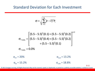
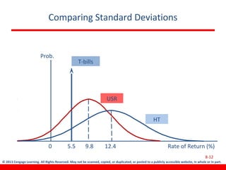
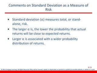
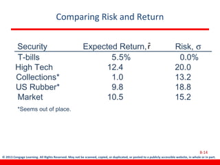
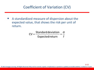
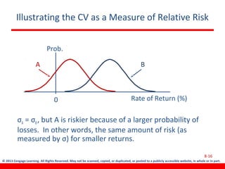
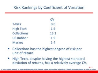
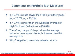
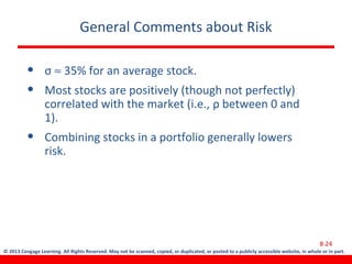
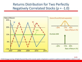
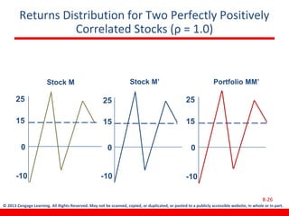
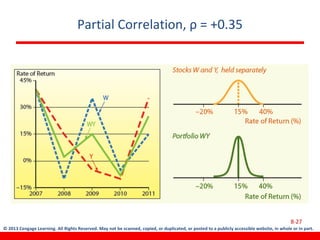
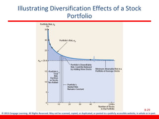
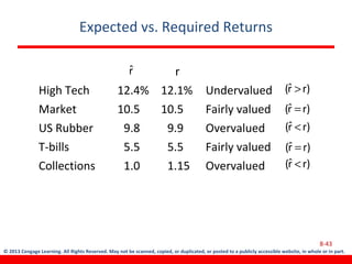
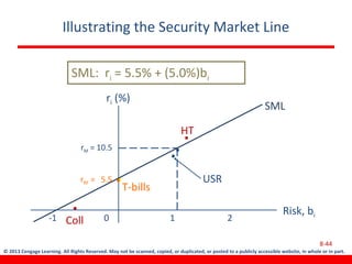
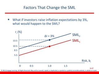
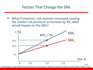
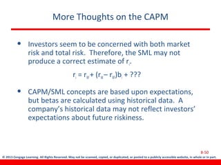
More Related Content
Similar to Bh ffm13 ppt_ch08
Similar to Bh ffm13 ppt_ch08 (20)
Bh ffm13 ppt_ch08
- 1. © 2013 Cengage Learning. All Rights Reserved. May not be scanned, copied, or duplicated, or posted to a publicly accessible website, in whole or in part.
Risk and Rates of Return
Stand-Alone Risk
Portfolio Risk
Risk and Return: CAPM/SML
Chapter 8
8-1
- 2. © 2013 Cengage Learning. All Rights Reserved. May not be scanned, copied, or duplicated, or posted to a publicly accessible website, in whole or in part.
What is investment risk?
• Two types of investment risk
– Stand-alone risk
– Portfolio risk
• Investment risk is related to the probability of
earning a low or negative actual return.
• The greater the chance of lower than expected, or
negative returns, the riskier the investment.
8-2
- 3. © 2013 Cengage Learning. All Rights Reserved. May not be scanned, copied, or duplicated, or posted to a publicly accessible website, in whole or in part.
Probability Distributions
• A listing of all possible outcomes, and the
probability of each occurrence.
• Can be shown graphically.
8-3
Expected Rate of Return
Rate of
Return (%)100150-70
Firm X
Firm Y
- 4. © 2013 Cengage Learning. All Rights Reserved. May not be scanned, copied, or duplicated, or posted to a publicly accessible website, in whole or in part.
Selected Realized Returns, 1926-2010
Source: Based on Ibbotson Stocks, Bonds, Bills, and Inflation: 2011 Classic
Yearbook (Chicago: Morningstar, Inc., 2011), p. 32.
8-4
- 5. © 2013 Cengage Learning. All Rights Reserved. May not be scanned, copied, or duplicated, or posted to a publicly accessible website, in whole or in part.
Hypothetical Investment Alternatives
Economy Prob
.
T-Bills HT Coll USR MP
Recession 0.1 5.5% -27.0% 27.0% 6.0% -17.0%
Below avg 0.2 5.5% -7.0% 13.0% -14.0% -3.0%
Average 0.4 5.5% 15.0% 0.0% 3.0% 10.0%
Above avg 0.2 5.5% 30.0% -11.0% 41.0% 25.0%
Boom 0.1 5.5% 45.0% -21.0% 26.0% 38.0%
8-5
- 6. © 2013 Cengage Learning. All Rights Reserved. May not be scanned, copied, or duplicated, or posted to a publicly accessible website, in whole or in part.
Why is the T-bill return independent of the economy?
Do T-bills promise a completely risk-free return?
• T-bills will return the promised 5.5%, regardless of
the economy.
• No, T-bills do not provide a completely risk-free
return, as they are still exposed to inflation.
Although, very little unexpected inflation is likely to
occur over such a short period of time.
• T-bills are also risky in terms of reinvestment risk.
• T-bills are risk-free in the default sense of the word.
8-6
- 7. © 2013 Cengage Learning. All Rights Reserved. May not be scanned, copied, or duplicated, or posted to a publicly accessible website, in whole or in part.
How do the returns of High Tech and Collections
behave in relation to the market?
• High Tech: Moves with the economy, and has a
positive correlation. This is typical.
• Collections: Is countercyclical with the economy,
and has a negative correlation. This is unusual.
8-7
- 8. © 2013 Cengage Learning. All Rights Reserved. May not be scanned, copied, or duplicated, or posted to a publicly accessible website, in whole or in part.
Calculating the Expected Return
8-8
12.4%
(0.1)(45%)(0.2)(30%)
(0.4)(15%)(0.2)(-7%)-27%))(1.0(rˆ
rPrˆ
returnofrateExpectedrˆ
N
1i
ii
=
++
++=
=
=
∑=
- 9. © 2013 Cengage Learning. All Rights Reserved. May not be scanned, copied, or duplicated, or posted to a publicly accessible website, in whole or in part.
Summary of Expected Returns
Expected Return
High Tech 12.4%
Market 10.5%
US Rubber 9.8%
T-bills 5.5%
Collections 1.0%
High Tech has the highest expected return, and
appears to be the best investment alternative, but is it
really? Have we failed to account for risk?
8-9
- 10. © 2013 Cengage Learning. All Rights Reserved. May not be scanned, copied, or duplicated, or posted to a publicly accessible website, in whole or in part.
Calculating Standard Deviation
8-10
∑=
−=σ
σ==σ
=σ
N
1i
i
2
2
P)rˆr(
Variance
deviationStandard
- 11. © 2013 Cengage Learning. All Rights Reserved. May not be scanned, copied, or duplicated, or posted to a publicly accessible website, in whole or in part.
Standard Deviation for Each Investment
8-11
%0.0
)1.0()5.55.5(
)2.0()5.55.5()4.0()5.55.5(
)2.0()5.55.5()1.0()5.55.5(
P)rˆr(
bills-T
2/1
2
22
22
bills-T
N
1i
i
2
=σ
−+
−+−
−+−
=σ
−=σ ∑=
σM = 15.2% σUSR = 18.8%
σColl = 13.2%σHT = 20%
- 12. © 2013 Cengage Learning. All Rights Reserved. May not be scanned, copied, or duplicated, or posted to a publicly accessible website, in whole or in part.
Comparing Standard Deviations
8-12
USR
Prob.
T-bills
HT
0 5.5 9.8 12.4 Rate of Return (%)
- 13. © 2013 Cengage Learning. All Rights Reserved. May not be scanned, copied, or duplicated, or posted to a publicly accessible website, in whole or in part.
Comments on Standard Deviation as a Measure of
Risk
• Standard deviation (σi) measures total, or stand-
alone, risk.
• The larger σi is, the lower the probability that actual
returns will be close to expected returns.
• Larger σi is associated with a wider probability
distribution of returns.
8-13
- 14. © 2013 Cengage Learning. All Rights Reserved. May not be scanned, copied, or duplicated, or posted to a publicly accessible website, in whole or in part.
Comparing Risk and Return
8-14
Security Expected Return, Risk, σ
T-bills 5.5% 0.0%
High Tech 12.4 20.0
Collections* 1.0 13.2
US Rubber* 9.8 18.8
Market 10.5 15.2
*Seems out of place.
rˆ
- 15. © 2013 Cengage Learning. All Rights Reserved. May not be scanned, copied, or duplicated, or posted to a publicly accessible website, in whole or in part.
Coefficient of Variation (CV)
• A standardized measure of dispersion about the
expected value, that shows the risk per unit of
return.
8-15
rˆreturnExpected
deviationStandard
CV
σ
==
- 16. © 2013 Cengage Learning. All Rights Reserved. May not be scanned, copied, or duplicated, or posted to a publicly accessible website, in whole or in part.
Illustrating the CV as a Measure of Relative Risk
σA = σB, but A is riskier because of a larger probability of
losses. In other words, the same amount of risk (as
measured by σ) for smaller returns.
8-16
0
A B
Rate of Return (%)
Prob.
- 17. © 2013 Cengage Learning. All Rights Reserved. May not be scanned, copied, or duplicated, or posted to a publicly accessible website, in whole or in part.
Risk Rankings by Coefficient of Variation
CV
T-bills 0.0
High Tech 1.6
Collections 13.2
US Rubber 1.9
Market 1.4
• Collections has the highest degree of risk per
unit of return.
• High Tech, despite having the highest standard
deviation of returns, has a relatively average CV.
8-17
- 18. © 2013 Cengage Learning. All Rights Reserved. May not be scanned, copied, or duplicated, or posted to a publicly accessible website, in whole or in part.
Investor Attitude Towards Risk
• Risk aversion: assumes investors dislike risk and
require higher rates of return to encourage them to
hold riskier securities.
• Risk premium: the difference between the return
on a risky asset and a riskless asset, which serves as
compensation for investors to hold riskier
securities.
8-18
- 19. © 2013 Cengage Learning. All Rights Reserved. May not be scanned, copied, or duplicated, or posted to a publicly accessible website, in whole or in part.
Portfolio Construction: Risk and Return
• Assume a two-stock portfolio is created with $50,000
invested in both High Tech and Collections.
• A portfolio’s expected return is a weighted average of
the returns of the portfolio’s component assets.
• Standard deviation is a little more tricky and requires
that a new probability distribution for the portfolio
returns be constructed.
8-19
- 20. © 2013 Cengage Learning. All Rights Reserved. May not be scanned, copied, or duplicated, or posted to a publicly accessible website, in whole or in part.
Calculating Portfolio Expected Return
8-20
%7.6%)0.1(5.0%)4.12(5.0rˆ
rˆwrˆ
:averageweightedaisrˆ
p
N
1i
iip
p
=+=
= ∑=
- 21. © 2013 Cengage Learning. All Rights Reserved. May not be scanned, copied, or duplicated, or posted to a publicly accessible website, in whole or in part.
An Alternative Method for Determining
Portfolio Expected Return
Economy Prob HT Coll Port
Recession 0.1 -27.0% 27.0% 0.0%
Below avg 0.2 -7.0% 13.0% 3.0%
Average 0.4 15.0% 0.0% 7.5%
Above avg 0.2 30.0% -11.0% 9.5%
Boom 0.1 45.0% -21.0% 12.0%
8-21
6.7%(12.0%)0.10(9.5%)0.20
(7.5%)0.40(3.0%)0.20(0.0%)0.10rˆp
=++
++=
- 22. © 2013 Cengage Learning. All Rights Reserved. May not be scanned, copied, or duplicated, or posted to a publicly accessible website, in whole or in part.
Calculating Portfolio Standard Deviation and CV
8-22
51.0
%7.6
%4.3
CV
%4.3
6.7)-(12.00.10
6.7)-(9.50.20
6.7)-(7.50.40
6.7)-(3.00.20
6.7)-(0.00.10
p
2
1
2
2
2
2
2
p
==
=
+
+
+
+
=σ
- 23. © 2013 Cengage Learning. All Rights Reserved. May not be scanned, copied, or duplicated, or posted to a publicly accessible website, in whole or in part.
Comments on Portfolio Risk Measures
• σp = 3.4% is much lower than the σi of either stock
(σHT = 20.0%; σColl = 13.2%).
• σp = 3.4% is lower than the weighted average of
High Tech and Collections’ σ (16.6%).
• Therefore, the portfolio provides the average
return of component stocks, but lower than the
average risk.
• Why? Negative correlation between stocks.
8-23
- 24. © 2013 Cengage Learning. All Rights Reserved. May not be scanned, copied, or duplicated, or posted to a publicly accessible website, in whole or in part.
General Comments about Risk
• σ ≈ 35% for an average stock.
• Most stocks are positively (though not perfectly)
correlated with the market (i.e., ρ between 0 and
1).
• Combining stocks in a portfolio generally lowers
risk.
8-24
- 25. © 2013 Cengage Learning. All Rights Reserved. May not be scanned, copied, or duplicated, or posted to a publicly accessible website, in whole or in part.
Returns Distribution for Two Perfectly
Negatively Correlated Stocks (ρ = -1.0)
8-25
- 26. © 2013 Cengage Learning. All Rights Reserved. May not be scanned, copied, or duplicated, or posted to a publicly accessible website, in whole or in part.
Returns Distribution for Two Perfectly Positively
Correlated Stocks (ρ = 1.0)
8-26
Stock M
0
15
25
-10
Stock M’
0
15
25
-10
Portfolio MM’
0
15
25
-10
- 27. © 2013 Cengage Learning. All Rights Reserved. May not be scanned, copied, or duplicated, or posted to a publicly accessible website, in whole or in part.
Partial Correlation, ρ = +0.35
8-27
- 28. © 2013 Cengage Learning. All Rights Reserved. May not be scanned, copied, or duplicated, or posted to a publicly accessible website, in whole or in part.
Creating a Portfolio: Beginning with One Stock and
Adding Randomly Selected Stocks to Portfolio
• σp decreases as stocks are added, because they
would not be perfectly correlated with the
existing portfolio.
• Expected return of the portfolio would remain
relatively constant.
• Eventually the diversification benefits of adding
more stocks dissipates (after about 40 stocks),
and for large stock portfolios, σp tends to
converge to ≈ 20%.
8-28
- 29. © 2013 Cengage Learning. All Rights Reserved. May not be scanned, copied, or duplicated, or posted to a publicly accessible website, in whole or in part.
Illustrating Diversification Effects of a Stock
Portfolio
8-29
- 30. © 2013 Cengage Learning. All Rights Reserved. May not be scanned, copied, or duplicated, or posted to a publicly accessible website, in whole or in part.
Breaking Down Sources of Risk
Stand-alone risk = Market risk + Diversifiable risk
• Market risk: portion of a security’s stand-alone risk
that cannot be eliminated through diversification.
Measured by beta.
• Diversifiable risk: portion of a security’s stand-
alone risk that can be eliminated through proper
diversification.
8-30
- 31. © 2013 Cengage Learning. All Rights Reserved. May not be scanned, copied, or duplicated, or posted to a publicly accessible website, in whole or in part.
Failure to Diversify
• If an investor chooses to hold a one-stock portfolio
(doesn’t diversify), would the investor be
compensated for the extra risk they bear?
– NO!
– Stand-alone risk is not important to a well-diversified
investor.
– Rational, risk-averse investors are concerned with σp,
which is based upon market risk.
– There can be only one price (the market return) for a
given security.
– No compensation should be earned for holding
unnecessary, diversifiable risk.
8-31
- 32. © 2013 Cengage Learning. All Rights Reserved. May not be scanned, copied, or duplicated, or posted to a publicly accessible website, in whole or in part.
Capital Asset Pricing Model (CAPM)
• Model linking risk and required returns. CAPM
suggests that there is a Security Market Line (SML)
that states that a stock’s required return equals the
risk-free return plus a risk premium that reflects the
stock’s risk after diversification.
ri = rRF+ (rM– rRF)bi
• Primary conclusion: The relevant riskiness of a stock
is its contribution to the riskiness of a well-
diversified portfolio.
8-32
- 33. © 2013 Cengage Learning. All Rights Reserved. May not be scanned, copied, or duplicated, or posted to a publicly accessible website, in whole or in part.
Beta
• Measures a stock’s market risk, and shows a stock’s
volatility relative to the market.
• Indicates how risky a stock is if the stock is held in a
well-diversified portfolio.
8-33
- 34. © 2013 Cengage Learning. All Rights Reserved. May not be scanned, copied, or duplicated, or posted to a publicly accessible website, in whole or in part.
Comments on Beta
• If beta = 1.0, the security is just as risky as the
average stock.
• If beta > 1.0, the security is riskier than average.
• If beta < 1.0, the security is less risky than average.
• Most stocks have betas in the range of 0.5 to 1.5.
8-34
- 35. © 2013 Cengage Learning. All Rights Reserved. May not be scanned, copied, or duplicated, or posted to a publicly accessible website, in whole or in part.
Can the beta of a security be negative?
• Yes, if the correlation between Stock i and the
market is negative (i.e., ρi,m < 0).
• If the correlation is negative, the regression line
would slope downward, and the beta would be
negative.
• However, a negative beta is highly unlikely.
8-35
- 36. © 2013 Cengage Learning. All Rights Reserved. May not be scanned, copied, or duplicated, or posted to a publicly accessible website, in whole or in part.
Calculating Betas
• Well-diversified investors are primarily concerned
with how a stock is expected to move relative to
the market in the future.
• Without a crystal ball to predict the future, analysts
are forced to rely on historical data. A typical
approach to estimate beta is to run a regression of
the security’s past returns against the past returns
of the market.
• The slope of the regression line is defined as the
beta coefficient for the security.
8-36
- 37. © 2013 Cengage Learning. All Rights Reserved. May not be scanned, copied, or duplicated, or posted to a publicly accessible website, in whole or in part.
Illustrating the Calculation of Beta
8-37
.
.
.
ri
_
rM
-5 0 5 10 15 20
20
15
10
5
-5
-10
Regression line:
ri = -2.59 + 1.44 rM
^ ^
Year rM ri
1 15% 18%
2 -5 -10
3 12 16
- 38. © 2013 Cengage Learning. All Rights Reserved. May not be scanned, copied, or duplicated, or posted to a publicly accessible website, in whole or in part.
Beta Coefficients for High Tech, Collections, and
T-Bills
8-38
rM
ri
-20 0 20 40
40
20
-20
HT: b = 1.32
T-bills: b = 0
Coll: b = -0.87
- 39. © 2013 Cengage Learning. All Rights Reserved. May not be scanned, copied, or duplicated, or posted to a publicly accessible website, in whole or in part.
Comparing Expected Returns and Beta Coefficients
Security Expected Return Beta
High Tech 12.4% 1.32
Market 10.5 1.00
US Rubber 9.8 0.88
T-Bills 5.5 0.00
Collections 1.0 -0.87
Riskier securities have higher returns, so the rank
order is OK.
8-39
- 40. © 2013 Cengage Learning. All Rights Reserved. May not be scanned, copied, or duplicated, or posted to a publicly accessible website, in whole or in part.
The Security Market Line (SML): Calculating
Required Rates of Return
SML: ri = rRF+ (rM– rRF)bi
ri = rRF+ (RPM)bi
• Assume the yield curve is flat and that rRF= 5.5% and
RPM= rM − rRF = 10.5% − 5.5% = 5.0%.
8-40
- 41. © 2013 Cengage Learning. All Rights Reserved. May not be scanned, copied, or duplicated, or posted to a publicly accessible website, in whole or in part.
What is the market risk premium?
• Additional return over the risk-free rate needed to
compensate investors for assuming an average
amount of risk.
• Its size depends on the perceived risk of the stock
market and investors’ degree of risk aversion.
• Varies from year to year, but most estimates
suggest that it ranges between 4% and 8% per year.
8-41
- 42. © 2013 Cengage Learning. All Rights Reserved. May not be scanned, copied, or duplicated, or posted to a publicly accessible website, in whole or in part.
Calculating Required Rates of Return
8-42
rHT = 5.5% + (5.0%)(1.32)
= 5.5% + 6.6% = 12.10%
rM = 5.5% + (5.0%)(1.00) = 10.50%
rUSR = 5.5% +(5.0%)(0.88) = 9.90%
rT-bill = 5.5% + (5.0)(0.00) = 5.50%
rColl = 5.5% + (5.0%)(-0.87) = 1.15%
- 43. © 2013 Cengage Learning. All Rights Reserved. May not be scanned, copied, or duplicated, or posted to a publicly accessible website, in whole or in part.
r
High Tech 12.4% 12.1% Undervalued
Market 10.5 10.5 Fairly valued
US Rubber 9.8 9.9 Overvalued
T-bills 5.5 5.5 Fairly valued
Collections 1.0 1.15 Overvalued
Expected vs. Required Returns
8-43
rˆ
)rrˆ( >
)rrˆ( =
)rrˆ( <
)rrˆ( =
)rrˆ( <
- 44. © 2013 Cengage Learning. All Rights Reserved. May not be scanned, copied, or duplicated, or posted to a publicly accessible website, in whole or in part.
Illustrating the Security Market Line
8-44
.
.
Coll
.HT
T-bills
.
USR
SML
rM = 10.5
rRF = 5.5
-1 0 1 2
.
SML: ri = 5.5% + (5.0%)bi
ri (%)
Risk, bi
.
- 45. © 2013 Cengage Learning. All Rights Reserved. May not be scanned, copied, or duplicated, or posted to a publicly accessible website, in whole or in part.
An Example:
Equally-Weighted Two-Stock Portfolio
• Create a portfolio with 50% invested in High Tech
and 50% invested in Collections.
• The beta of a portfolio is the weighted average of
each of the stock’s betas.
bP = wHTbHT + wCollbColl
bP = 0.5(1.32) + 0.5(-0.87)
bP = 0.225
8-45
- 46. © 2013 Cengage Learning. All Rights Reserved. May not be scanned, copied, or duplicated, or posted to a publicly accessible website, in whole or in part.
Calculating Portfolio Required Returns
• The required return of a portfolio is the weighted
average of each of the stock’s required returns.
rP = wHTrHT + wCollrColl
rP = 0.5(12.10%) + 0.5(1.15%)
rP = 6.625%
• Or, using the portfolio’s beta, CAPM can be used to
solve for expected return.
rP = rRF+ (RPM)bP
rP = 5.5%+ (5.0%)(0.225)
rP = 6.625%
8-46
- 47. © 2013 Cengage Learning. All Rights Reserved. May not be scanned, copied, or duplicated, or posted to a publicly accessible website, in whole or in part.
Factors That Change the SML
• What if investors raise inflation expectations by 3%,
what would happen to the SML?
8-47
SML1
ri (%)
SML2
0 0.5 1.0 1.5
13.5
10.5
8.5
5.5
ΔI = 3%
Risk, bi
- 48. © 2013 Cengage Learning. All Rights Reserved. May not be scanned, copied, or duplicated, or posted to a publicly accessible website, in whole or in part.
Factors That Change the SML
• What if investors’ risk aversion increased, causing
the market risk premium to increase by 3%, what
would happen to the SML?
8-48
SML1
ri (%) SML2
0 0.5 1.0 1.5
ΔRPM = 3%
Risk, bi
13.5
10.5
5.5
- 49. © 2013 Cengage Learning. All Rights Reserved. May not be scanned, copied, or duplicated, or posted to a publicly accessible website, in whole or in part.
Verifying the CAPM Empirically
• The CAPM has not been verified completely.
• Statistical tests have problems that make
verification almost impossible.
• Some argue that there are additional risk factors,
other than the market risk premium, that must be
considered.
8-49
- 50. © 2013 Cengage Learning. All Rights Reserved. May not be scanned, copied, or duplicated, or posted to a publicly accessible website, in whole or in part.
More Thoughts on the CAPM
• Investors seem to be concerned with both market
risk and total risk. Therefore, the SML may not
produce a correct estimate of ri.
ri = rRF+ (rM– rRF)bi + ???
• CAPM/SML concepts are based upon expectations,
but betas are calculated using historical data. A
company’s historical data may not reflect investors’
expectations about future riskiness.
8-50