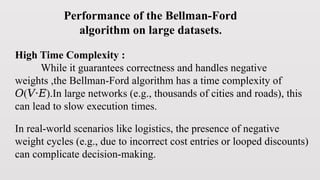
The Bellman-Ford algorithm, developed by Richard Bellman, is a dynamic programming technique used to find the shortest paths from a single source vertex to all other vertices in a weighted graph, capable of handling negative weights and detecting negative cycles. The algorithm operates through edge relaxation and iterates V-1 times, followed by a check for negative cycles. Its applications are critical in scenarios such as logistics for determining optimal delivery paths, though it is considered slow for larger graphs due to its high time complexity.

1. BELLMAN-FORD
ALGORITHM
23I304-DATA STRUCTURES
ARCHANA-23I307 SAKTHISREE-23I350
MOUNIKA-23I334 SELVA MITHRA-23I356
PREETHI-23I344 SHREAYAA-23I359

2. INTRODUCTION
• BELLMAN ALGORITHM WAS FIRST PROPOSED BY LESTER
FORD IN 1956 AND LATER IMPROVED BY RICHARD
BELLMAN IN 1958.
• IT IS A DYNAMIC PROGRAMMING ALGORITHM USED TO FIND
SHORTEST PATH FROM SINGLE SOURCE VERTEX TO ALL OTHER
VERTICES IN A WEIGHTED GRAPH.
• IT CAN DEAL WITH NEGATIVE CYCLE i.e, IT CAN DETECT
NEGATIVE CYCLE.

3. HOW DOES IT WORKS??
• IT WORKS BY RELAXING THE EDGES OF THE GRAPH
REPEATEDLY.
• RELAXATION INVOLVES UPDATING THE DISTANCE TO VERTEX IF
A SHORTER PATH IS FOUND.
• THE ALGORITHM ITERATES TO ALL EDGES V-1TIMES,WHERE V IS
NUMBER OF VERTICES.
• IF THE DISTANCE TO ANY VERTEX CAN STILL BE REDUCED AFTER
V-1 ITERATIONS,THEN THE GRAPH CONTAINS A NEGATIVE CYCLE.

4. APPLICATIONS

5. ADVANTAGES:
• HANDLES NEGATIVE WEIGHTS.
• DETECTS NEGATIVE CYCLES.
• SIMPLE TO IMPLEMENT.
DISADVANTAGES:
• SLOW FOR LARGE GRAPHS.
• REQUIRES MULTIPLE ITERATIONS.

6. ALGORITHM
1. Set source vertex distance to 0
Set all other vertex distance as infinity
2. Relax all edges
2.1 Write all the edges in any order
2.2 Relax the edges
2.3 Repeat for V-1 times.
3. Check for negative weight cycle by relaxing again and
checking for changes.
4. Shortest distance from source to all vertex is determined.

8. Example Graph :

9. 0 ∞
∞
∞
∞
STEP 1:

10. STEP 2:
ORDER OF EDGES:
1. (2,4) 4. (3,1)
2. (4,3) 5.(1,2)
3. (0,2) 6.(2,3)
7. (0,1)

11. 0
∞
∞
∞
∞
2
6
-1
STEP 3:
* Relax the edges for 3 more times
ORDER OF EDGES:
1. (2,4) 4. (3,1)
2. (4,3) 5.(1,2)
3. (0,2) 6.(2,3)
7. (0,1)

12. STEP 4:
0 0
3
4
-1

13. BASIC CODE

15. Initial distances Array:
distances=[0, ∞, ∞]
distances=float(‘inf’)*V ∞*no of vertices(3)
distances[source] = 0
distances=[∞, ∞, ∞]
distances[0] = 0 (i.e source is 0)
Input:
Enter the number of vertices: 3
Enter the number of edges: 3
Enter edge (source destination weight): 0 1 4
Enter edge (source destination weight): 0 2 1
Enter edge (source destination weight): 1 2 -2
Enter the source vertex: 0
graph=[(0, 1, 4), (0, 2, 1), (1, 2, -2)]

16. Relaxing the edges v-1 times:
First Iteration (i = 1):
Edge (0 → 1, 4):
∙ Current distances: [0, ∞, ∞]
∙ distances[0] + weight = 0 + 4 = 4
∙ Compare with distances[1] (∞):
Update distances[1] to 4.
∙ Updated distances: [0, 4, ∞]
Edge (0 → 2, 1):
∙ Current distances: [0, 4, ∞]
∙ distances[0] + weight = 0 + 1 = 1
∙ Compare with distances[2] (∞):
Update distances[2] to 1.
∙ Updated distances: [0, 4, 1]
Edge (1 → 2, -2):
∙ Current distances: [0, 4, 1]
∙ distances[1] + weight = 4 + (-2) = 2
Compare with distances[2] (1):
No update, as 2 is greater than 1
After the first iteration:
distances: [0, 4, 1]

17. Second Iteration (i = 2):
We process all edges again:
Edge (0 → 1, 4):
∙ Current distances: [0, 4, 1]
∙ distances[0] + weight = 0 + 4 = 4
Compare with distances[1] (4):
No update, as they are equal
Edge (0 → 2, 1):
∙ Current distances: [0, 4, 1]
∙ distances[0] + weight = 0 + 1 = 1
∙ Compare with distances[2] (1):
No update, as they are equal.
Edge (1 → 2, -2):
•Current distances: [0, 4, 1]
•distances[1] + weight = 4 + (-2) = 2
•Compare with distances[2] (1):
No update, as 2 is greater than 1.
After the second iteration:
distances: [0, 4, 1]

18. •After relaxing all edges V-1 times, this step checks if any edge can still be
relaxed (which would indicate a negative weight cycle).
•If distances[u] + weight < distances[v] still holds for any edge, it means the
graph contains a negative weight cycle, and the algorithm prints a message and exits
Output:
Shortest distances from source:
Vertex 0: 0
Vertex 1: 4
Vertex 2: 1
Check for negative cycle:

19. Time complexity for all the three cases
For dense graphs:
Best Case: O(V²).
Average/Worst Case: O(V³) (if E ≈ V²).

20. You are working as a backend software engineer for a logistics company that
manages a large fleet of delivery trucks across a network of cities. The company
needs to determine the shortest path from a central warehouse to each delivery
destination. The cities are connected by roads, and each road has a specific travel
time (weight). Some roads may be one-way, while others are two-way. Additionally,
some cities might be connected by roads that can be traversed in either direction,
while other roads might have negative travel times due to certain conditions (e.g., toll
discounts during specific hours).
Given the nature of this dynamic network of cities and roads, the task is to compute
the shortest path from a single source city (the central warehouse) to all other cities
using the Bellman-Ford algorithm. The algorithm must handle the possibility of
negative weights and detect negative weight cycles in the network, which might
indicate an anomaly or issue in the road data.
CASE STUDY

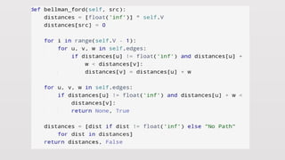
21. CASE STUDY CODE
def bellmanFord(V, edges, src):
INF = float('inf')
dist = [INF] * V
dist[src] = 0
for i in range(V):
for edge in edges:
u, v, wt = edge
if dist[u] != INF and dist[u] + wt < dist[v]:
if i == V - 1:
return [-1]
dist[v] = dist[u] + wt
return dist

22. print("Welcome to the Logistics Network Optimizer!")
V = int(input("Enter the number of cities: "))
E = int(input("Enter the number of roads: "))
print("nEnter the road details (source, destination, travel
time):")
edges = []
for i in range(E):
print(f"Road {i + 1}:")
u = int(input(" Source city (0-indexed): "))
v = int(input(" Destination city (0-indexed): "))
wt = int(input(" Travel time (can be negative): "))
edges.append([u, v, wt])

23. src = int(input("nEnter the source city (central warehouse, 0-
indexed): "))
print("nCalculating shortest paths...")
ans = bellmanFord(V, edges, src)
if ans == [-1]:
print("nError: Negative weight cycle detected in the network!")
else:
print("nShortest distances from the central warehouse:")
for city in range(V):
if ans[city] == float('inf'):
print(f" City {city}: No path available")
else:
print(f" City {city}: {ans[city]} time units")

24. OUTPUT:
Welcome to the Logistics Network Optimizer!
Enter the number of cities: 5
Enter the number of roads: 6
Enter the road details (source, destination, travel time):
Road 1:
Source city (0-indexed): 1
Destination city (0-indexed): 3
Travel time (can be negative): 2
Road 2:
Source city (0-indexed): 4 Destination city (0-indexed): 3
Travel time (can be negative): -1

25. Road 3:
Source city (0-indexed): 2
Destination city (0-indexed): 4
Travel time (can be negative): 1
Road 4:
Source city (0-indexed): 1
Destination city (0-indexed): 2
Travel time (can be negative): 1
Road 5:
Source city (0-indexed): 0
Destination city (0-indexed): 1
Travel time (can be negative): 5
Road 6:
Source city (0-indexed): 2
Destination city (0-indexed): 3
Travel time (can be negative): -5
Enter the source city (central warehouse,
0-indexed): 0
Calculating shortest paths...
Shortest distances from the central
warehouse:
City 0: 0 time units
City 1: 5 time units
City 2: 6 time units
City 3: 1 time units
City 4: 7 time units

26. CHALLENGES
Detection of negative weight cycle
- Initialization
- Relaxation
- Detection : After v-1 iterations, an additional iteration is
performed over all edges to detect negative weight
cycle. If a shorter path is still found, it means a negative
weight cycle exists.
Special cases handled
- No path exists between some cities.
- Multiple roads between the same pair of cities.
- Roads with zero weight.

28. ▪ Edges: 2,3,4
distances=[0, ∞, ∞]
After 1st
iteration : distances=[-2,5,8]
After 2nd
iteration : distances=[-4,3,6]
▪ Cycle Detection(additional iteration):
Edge in Focus: 2→4.
▪ If distances[2] + w < distances[4]
If -4+5<3
1<3 #returns true
▪ Output: Negative weight cycle detected!

29. Performance of the Bellman-Ford
algorithm on large datasets.
High Time Complexity :
While it guarantees correctness and handles negative
weights ,the Bellman-Ford algorithm has a time complexity of
( ).In large networks (e.g., thousands of cities and roads), this
𝑂 𝑉⋅𝐸
can lead to slow execution times.
In real-world scenarios like logistics, the presence of negative
weight cycles (e.g., due to incorrect cost entries or looped discounts)
can complicate decision-making.

30. TELECOMMUNICATION FAULT
DETECTION
1.Problem Overview
✔ Telecommunication networks
✔ Network consists of routers,
switches and hubs.
✔ Algorithm evaluates network
performance issues.
2. Graph Representation
✔ Nodes: Routers
✔ Edges: Communication
links.
✔ Edge weights:
Transmission costs.
✔ Negative edge weights:
Reduced bandwidth, faults,
or failures.

31. 3. Bellman-Ford’s Role
✔ Identifies the most efficient and
shortest path and minimizes
transmission cost.
✔ Negative Weight Cycles: Detects
unstable links or routing loops.
✔ Flagging Issues : Helps to flag
faulty links or misconfigured
routers to identify the cause.
4. Optimization techniques
✔ Preprocessing: Precompute
shortest path, periodic updates
✔ Distributed Bellman-Ford:
Parallelization

32. Conclusion
✔ Invaluable tool for fault detection
✔ Applicable for large-scale
✔ Preprocessing and distributed
computing reduces strain.
✔ To address computational overhead
problems, faster algorithms are
employed

33. PRACTICE MAKES PERFECT!
• https://leetcode.com/problems/cheapest-flights-within-k-stops/discuss/340911/understanding-
bellman-ford
• https://www.geeksforgeeks.org/problems/distance-from-the-source-bellman-ford-algorithm/1
REFERENCES
• https://www.geeksforgeeks.org/bellman-ford-algorithm-dp-23/
• https://en.wikipedia.org/wiki/Bellman%E2%80%93Ford_algorithm

34. THANK YOU