Visit: www.statisticsassignmenthelp.com
Email: support@statisticsassignmenthelp.com
Phone: +1 (315)-557-6473
Bayesian Inference and Maximum Likelihood
In this sample assignment, we explore a range of statistical problems to
illustrate the methods and techniques used in probability and estimation. This
exercise covers concepts such as the Method of Moments, Maximum
Likelihood Estimation (MLE), and Bayesian inference. The problems include
working with discrete random variables, geometric distributions, and
binomial distributions, highlighting their likelihood functions, parameter
estimation, and posterior distributions. Through these examples, the goal is to
showcase the practical application of statistical methods and the expertise of
StatisticsAssignmentHelp.com in solving complex assignments. Dive into
these challenges to gain a deeper understanding of advanced statistical
techniques.
Bayesian Inference and Maximum Likelihood
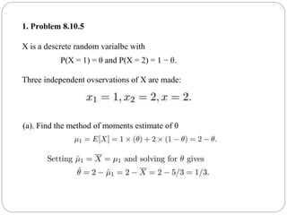
1. Problem 8.10.5
X is a descrete random varialbe with
P(X = 1) = θ and P(X = 2) = 1 − θ.
Three independent ovservations of X are made:
(a). Find the method of moments estimate of θ
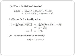
(b). What is the likelihood function?
(c).The mle for θ is found by solving
(d). The uniform distribution has density
The posterior distribution has density
By inspection, the posterior density must be that of a Beta(a, b) distribution
with
a = 2 and b = 3.
2. Problem 8.10.7
Suppose that X follows a geometric distribution
Assume an i.i.d. sample of size n.
(a). Find the method of moments estimate of p.
The first moment of X is
(See Appendex A, page A1.)
Solving gives
(b). Find the mle of p. The mle of a sample x1, . . . , xn minimizes
The mle is the same as the mle for a sample of size from a
Bernoulli(p) distribution with n successes:
(same as the method-of-moments estimate)
(c) The asympotic variance of the mle is
where
(d). Let p have a uniform distribution on [0, 1]. The posterior distribution
of p has density
which can be recognized as a Beta(a∗, b∗) distribution with
The mean of the posterior distribution is the mean of the Beta(a∗, b∗)
distribution which is
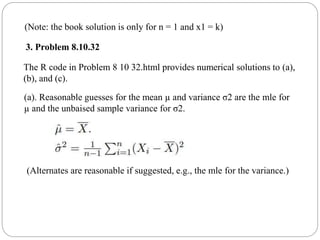
(Note: the book solution is only for n = 1 and x1 = k)
3. Problem 8.10.32
The R code in Problem 8 10 32.html provides numerical solutions to (a),
(b), and (c).
(a). Reasonable guesses for the mean µ and variance σ2 are the mle for
µ and the unbaised sample variance for σ2.
(Alternates are reasonable if suggested, e.g., the mle for the variance.)
(b). Confidence intervals for µ :
Let CI.level (×100%) be the confidence level of the interval.
Set α = 1 − CI.level and define t ∗ = t(α/2, df = (n − 1)), the upper α/2
quantile of a t distribution with n − 1 degrees of freedom. Then the
confidence interval for µ is
Confidence intervals for σ2 :
Let CI.level (×100%) be the confidence level of the interval.
(c). To compute confidence intervals for σ rather than σ2 , just take the
square roots of the corresponding confidence intervals for sigma2 .
(d). To halve the confidence interval for µ, the sample size should increase
about 4 times. The standard deviation of the sample mean is σ/ n so this is
halved when the sample size is increased by a factor of 4. This argument
does not account for the fact that the critical value of the t distribution of a
given α/2 level is smaller the higher the degrees of freedom. So, the factor
of 4 is an upper bound on the the sample size increase required. Also, the
length of the confidence interval for µ is random. The previous comments
apply on average, but in any sample, the confidence interval will have
random length and could be arbitrarily large, albeit with very small
probability.
4. Problem 8.10.63
Suppose that 100 items are sampled from a manufacturing process and 3
are found to be defective. Let X = 3 be the outcome of a Binomial(n =
100,θ) random variable.
The likelihood of the data is
Consider a prior distribution for θ which is Beta(a, b), (with a > 0,b > 0).
The posterior distribution has density:
Which normalizes to a Beta(a ∗,b∗) distribution where
a = a +3, and b∗ = b + 97.
The mean of the posterior distribution is
E[θ | X] = a ∗/(a + b∗).
For a = b = 1 we have E[θ | X] =4/102 and
For a.5, and b = 5 we have E[θ | X] = 3.5/105.5.
The R code in P roblem 8 10 63.html plots the prior/posterior densities
and computes the posterior means.

Bayesian Inference and Maximum Likelihood

  • 1.
    Visit: www.statisticsassignmenthelp.com Email: support@statisticsassignmenthelp.com Phone:+1 (315)-557-6473 Bayesian Inference and Maximum Likelihood
  • 2.
    In this sampleassignment, we explore a range of statistical problems to illustrate the methods and techniques used in probability and estimation. This exercise covers concepts such as the Method of Moments, Maximum Likelihood Estimation (MLE), and Bayesian inference. The problems include working with discrete random variables, geometric distributions, and binomial distributions, highlighting their likelihood functions, parameter estimation, and posterior distributions. Through these examples, the goal is to showcase the practical application of statistical methods and the expertise of StatisticsAssignmentHelp.com in solving complex assignments. Dive into these challenges to gain a deeper understanding of advanced statistical techniques. Bayesian Inference and Maximum Likelihood
  • 3.
    1. Problem 8.10.5 Xis a descrete random varialbe with P(X = 1) = θ and P(X = 2) = 1 − θ. Three independent ovservations of X are made: (a). Find the method of moments estimate of θ
  • 4.
    (b). What isthe likelihood function? (c).The mle for θ is found by solving (d). The uniform distribution has density
  • 5.
    The posterior distributionhas density By inspection, the posterior density must be that of a Beta(a, b) distribution with a = 2 and b = 3.
  • 6.
    2. Problem 8.10.7 Supposethat X follows a geometric distribution Assume an i.i.d. sample of size n. (a). Find the method of moments estimate of p. The first moment of X is
  • 7.
    (See Appendex A,page A1.) Solving gives (b). Find the mle of p. The mle of a sample x1, . . . , xn minimizes
  • 8.
    The mle isthe same as the mle for a sample of size from a Bernoulli(p) distribution with n successes: (same as the method-of-moments estimate) (c) The asympotic variance of the mle is where
  • 9.
    (d). Let phave a uniform distribution on [0, 1]. The posterior distribution of p has density which can be recognized as a Beta(a∗, b∗) distribution with The mean of the posterior distribution is the mean of the Beta(a∗, b∗) distribution which is
  • 10.
    (Note: the booksolution is only for n = 1 and x1 = k) 3. Problem 8.10.32 The R code in Problem 8 10 32.html provides numerical solutions to (a), (b), and (c). (a). Reasonable guesses for the mean µ and variance σ2 are the mle for µ and the unbaised sample variance for σ2. (Alternates are reasonable if suggested, e.g., the mle for the variance.)
  • 11.
    (b). Confidence intervalsfor µ : Let CI.level (×100%) be the confidence level of the interval. Set α = 1 − CI.level and define t ∗ = t(α/2, df = (n − 1)), the upper α/2 quantile of a t distribution with n − 1 degrees of freedom. Then the confidence interval for µ is Confidence intervals for σ2 : Let CI.level (×100%) be the confidence level of the interval.
  • 12.
    (c). To computeconfidence intervals for σ rather than σ2 , just take the square roots of the corresponding confidence intervals for sigma2 .
  • 13.
    (d). To halvethe confidence interval for µ, the sample size should increase about 4 times. The standard deviation of the sample mean is σ/ n so this is halved when the sample size is increased by a factor of 4. This argument does not account for the fact that the critical value of the t distribution of a given α/2 level is smaller the higher the degrees of freedom. So, the factor of 4 is an upper bound on the the sample size increase required. Also, the length of the confidence interval for µ is random. The previous comments apply on average, but in any sample, the confidence interval will have random length and could be arbitrarily large, albeit with very small probability.
  • 14.
    4. Problem 8.10.63 Supposethat 100 items are sampled from a manufacturing process and 3 are found to be defective. Let X = 3 be the outcome of a Binomial(n = 100,θ) random variable. The likelihood of the data is Consider a prior distribution for θ which is Beta(a, b), (with a > 0,b > 0).
  • 15.
    The posterior distributionhas density: Which normalizes to a Beta(a ∗,b∗) distribution where a = a +3, and b∗ = b + 97. The mean of the posterior distribution is E[θ | X] = a ∗/(a + b∗). For a = b = 1 we have E[θ | X] =4/102 and
  • 16.
    For a.5, andb = 5 we have E[θ | X] = 3.5/105.5. The R code in P roblem 8 10 63.html plots the prior/posterior densities and computes the posterior means.