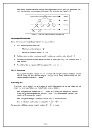
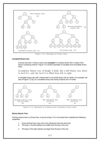
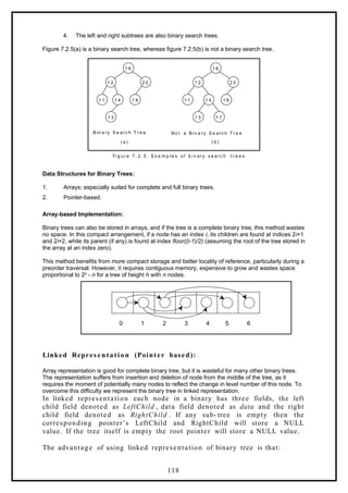
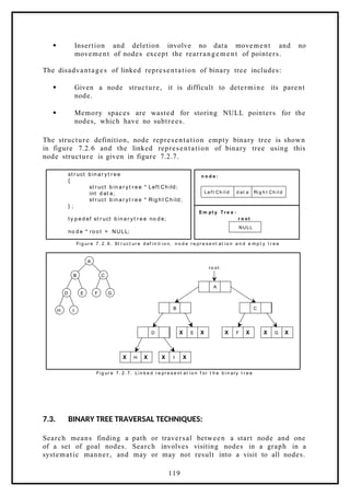
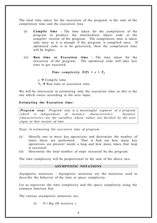
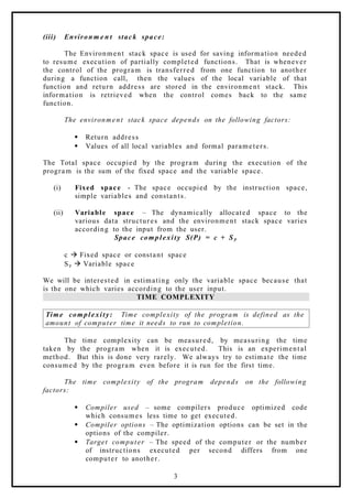
This document contains lecture notes on data structures that discuss programming performance, space complexity, time complexity, asymptotic notations, and searching and sorting algorithms. The key points covered are: - Programming performance is measured by the memory and time needed to run a program, which can be analyzed or experimentally measured. - Space complexity accounts for memory needed and includes instruction, data, and environment stack spaces. Time complexity accounts for time needed and includes compilation and execution times. - Common asymptotic notations like Big-O, Omega, and Theta are used to describe time and space complexity behaviors. - Searching algorithms like linear and binary search are used to find elements. Sorting algorithms like bubble, quick, selection and heap sorts

1. LECTURE NOTES
on
DATA STRUCTURES
2018 – 2019
I B. Tech II Semest er (R17)
Mr. K Munivara Prasad, Associate Professor
CHADALAWADA RAMANAMMA ENGINEERING COLLEGE
(AUTONOMOUS)
Chadalawada Nagar, Renigunta Road, Tirupati – 517 506
Department of Computer Science and Engineering
1

2. UNIT-I
PROGRAMMING PERFORMANCE
Perfor m a n c e of a progra m: The performance of a program is
measured based on the amount of computer memory and time needed
to run a program.
The two approaches which are used to measure the performance of the
program are:
1. Analytical meth o d à called the Performance Analysis.
2. Experim e n t al meth o d à called the Performance Measurement.
SPACE COMPLEXITY
Space complexity: The Space complexity of a program is defined as
the amount of memory it needs to run to completion.
As said above the space complexity is one of the factor which
accounts for the performance of the program. The space complexity can
be measured using experimental method, which is done by running the
program and then measuring the actual space occupied by the program
during execution. But this is done very rarely. We estimate the space
complexity of the program before running the program.
Space complexity is the sum of the following compon e n t s:
(i) Instruc tio n space:
The program which is written by the user is the source program.
When this program is compiled, a compiled version of the program is
generated. For executing the program an executable version of the
program is generated. The space occupied by these three when the
program is under execution, will account for the instruction space.
(ii) Data space:
The space needed by the constants, simple variables, arrays,
structures and other data structures will account for the data space.
The Data space depends on the following factors:
 Structure size – It is the sum of the size of component
variables of the structure.
 Array size – Total size of the array is the product of the size
of the data type and the number of array locations.
2

3. (iii) Environ m e n t stack space:
The Environment stack space is used for saving information needed
to resume execution of partially completed functions. That is whenever
the control of the program is transferred from one function to another
during a function call, then the values of the local variable of that
function and return address are stored in the environment stack. This
information is retrieved when the control comes back to the same
function.
The environment stack space depends on the following factors:
 Return address
 Values of all local variables and formal parameters.
The Total space occupied by the program during the execution of the
program is the sum of the fixed space and the variable space.
(i) Fixed space - The space occupied by the instruction space,
simple variables and constants.
(ii) Variable space – The dynamically allocated space to the
various data structures and the environment stack space varies
according to the input from the user.
Space complexity S(P) = c + S p
c à Fixed space or constant space
Sp à Variable space
We will be interested in estimating only the variable space because that
is the one which varies according to the user input.
TIME COMPLEXITY
Time compl exity: Time complexity of the program is defined as the
amount of computer time it needs to run to completion.
The time complexity can be measured, by measuring the time
taken by the program when it is executed. This is an experimental
method. But this is done very rarely. We always try to estimate the time
consumed by the program even before it is run for the first time.
The time complexity of the program depends on the following
factors:
 Compiler used – some compilers produce optimized code
which consumes less time to get executed.
 Compiler options – The optimization options can be set in the
options of the compiler.
 Target computer – The speed of the computer or the number
of instructions executed per second differs from one
computer to another.
3

4. The total time taken for the execution of the program is the sum of the
compilation time and the execution time.
(i) Compile time – The time taken for the compilation of the
program to produce the intermediate object code or the
compiler version of the program. The compilation time is taken
only once as it is enough if the program is compiled once. If
optimized code is to be generated, then the compilation time
will be higher.
(ii) Run time or Execution time - The time taken for the
execution of the program. The optimized code will take less
time to get executed.
Time compl exity T(P) = c + T p
c à Compile time
Tp à Run time or execution time
We will be interested in estimating only the execution time as this is the
one which varies according to the user input.
Estimatin g the Execution time:
Progra m step: Program step is a meaningful segment of a program
which is independent of instance characteristics. Instance
characteristics are the variables whose values are decided by the user
input at that instant of time.
Steps in estimating the execution time of program:
(i) Identify one or more key operations and determine the number of
times these are performed. That is find out how many key
operations are present inside a loop and how many times that loop
is executed.
(ii) Determine the total number of steps executed by the program.
The time complexity will be proportional to the sum of the above two.
ASYMPTOTIC NOTATIONS
Asymptotic notations – Asymptotic notations are the notations used to
describe the behavior of the time or space complexity.
Let us represent the time complexity and the space complexity using the
common function f(n).
The various asymptotic notations are:
(i) O ( Big Oh notation )
4

5. (ii) ( Omega notation )
Ω
(iii) ( Theta notation )
θ
(iv) o ( Little Oh notation )
O – Big Oh notation
The big Oh notation provides an upper bound for the function f(n).
The function f(n) = O(g(n)) if and only if there exists positive constants
c and n0 such that f(n) cg(n) for all n n
≤ ≥ 0.
Examples:
1. f(n) = 3n + 2
Let us take g(n) = n
c = 4
n0 = 2
Let us check the above condition
3n + 1 4n
≤ for all n 2
≥
The condition is satisfied. Hence f(n) = O(n).
2. f(n) = 10n 2 + 4n + 2
Let us take g(n) = n 2
c = 11
n0 = 6
Let us check the above condition
10n 2 + 4n + 2 11n
≤ for all n 6
≥
The condition is satisfied. Hence f(n) = O(n 2).
- Omega notation
Ω
The notation gives the lower bound for the function f(n).
Ω
The function f(n) = (g(n)) if and only if there exists positive constants
Ω
c and n0 such that f(n) cg(n) for all n n
≥ ≥ 0.
Examples:
1. f(n) = 3n + 2
Let us take g(n) = n
c = 3
n0 = 0
5

6. Let us check the above condition
3n + 1 3n
≥ for all n 0
≥
The condition is satisfied. Hence f(n) = (n).
Ω
2. f(n) = 10n 2 + 4n + 2
Let us take g(n) = n 2
c = 10
n0 = 0
Let us check the above condition
10n 2 + 4n + 2 10n
≥ for all n 0
≥
The condition is satisfied. Hence f(n) = (n
Ω 2).
– Theta notation
θ
The theta notation is used when the function f(n) can be bounded by both
from above and below the same function g(n).
f(n) = (g(n)) if and only if there exists some positive constants c
θ 1 and c2
and n0, such that c1g(n) f(n) c
≤ ≤ 2g(n) for all n n
≥ 0.
We have seen in the previous two cases,
3n + 2 = O(n) and 3n + 2 = (n)
Ω
Hence we can write 3n + 2 = (n)
θ
o - Little Oh notation
f(n) = o(g(n)) if and only if f(n) = O(g(n)) and f(n) (g(n))
≠ Ω
For example,
3n + 2 = O(n 2) but 3n + 2 (n
≠ Ω 2)
Therefore it can be written as 3n + 2 = o(n 2)
6

7. SEARCHING AND SORTING
Searching is used to find the location where an element is available. There are two types of search
techniques. They are:
1. Linear or sequential search
2. Binary search
Sorting allows an efficient arrangement of elements within a given data structure. It is a way in which
the elements are organized systematically for some purpose. For example, a dictionary in which
words are arranged in alphabetical order and telephone director in which the subscriber names are
listed in alphabetical order. There are many sorting techniques out of which we study the following.
1. Bubble sort
2. Quick sort
3. Selection sort and
4. Heap sort
LINEAR SEARCH
This is the simplest of all searching techniques. In this technique, an ordered or unordered list will be
searched one by one from the beginning until the desired element is found. If the desired element is
found in the list then the search is successful otherwise unsuccessful.
Suppose there are ‘n’ elements organized sequentially on a List. The number of comparisons
required to retrieve an element from the list, purely depends on where the element is stored in the list.
If it is the first element, one comparison will do; if it is second element two comparisons are necessary
and so on. On an average you need [(n+1)/2] comparison’s to search an element. If search is not
successful, you would need ’n’ comparisons.
The time complexity of linear search is O(n).
Algorithm:
Let array a[n] stores n elements. Determine whether element ‘x’ is present or not.
linsrch(a[n], x)
{
index = 0;
flag = 0;
while (index < n) do
{
if (x == a[index])
{
flag = 1;
break;
}
index ++;
}
if(flag == 1)
printf(“Data found at %d position“, index);
else
printf(“data not found”);
}
7

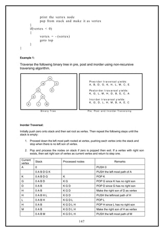
8. Example 1:
Suppose we have the following unsorted list: 45, 39, 8, 54, 77, 38, 24, 16, 4, 7, 9, 20
If we are searching for: 45, we’ll look at 1 element before success
39, we’ll look at 2 elements before success
8, we’ll look at 3 elements before success
54, we’ll look at 4 elements before success
77, we’ll look at 5 elements before success
38 we’ll look at 6 elements before success
24, we’ll look at 7 elements before success
16, we’ll look at 8 elements before success
4, we’ll look at 9 elements before success
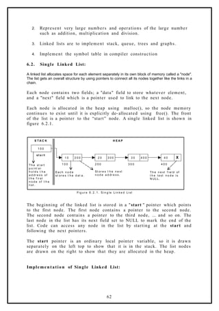
7, we’ll look at 10 elements before success
9, we’ll look at 11 elements before success
20, we’ll look at 12 elements before success
For any element not in the list, we’ll look at 12 elements before failure
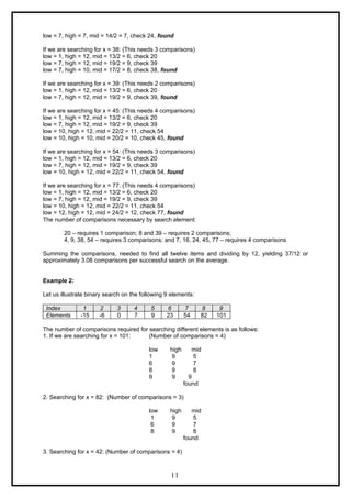
Example 2:
Let us illustrate linear search on the following 9 elements:
Index 0 1 2 3 4 5 6 7 8
Elements -15 -6 0 7 9 23 54 82 101
Searching different elements is as follows:
1. Searching for x = 7 Search successful, data found at 3rd
position
2. Searching for x = 82 Search successful, data found at 7th
position
3. Searching for x = 42 Search un-successful, data not found
A non-recursive program for Linear Search:
# include <stdio.h>
# include <conio.h>
main()
{
int number[25], n, data, i, flag = 0;
clrscr();
printf("n Enter the number of elements: ");
scanf("%d", &n);
printf("n Enter the elements: ");
for(i = 0; i < n; i++)
scanf("%d", &number[i]);
printf("n Enter the element to be Searched: ");
scanf("%d", &data);
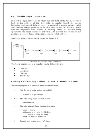
for( i = 0; i < n; i++)
{
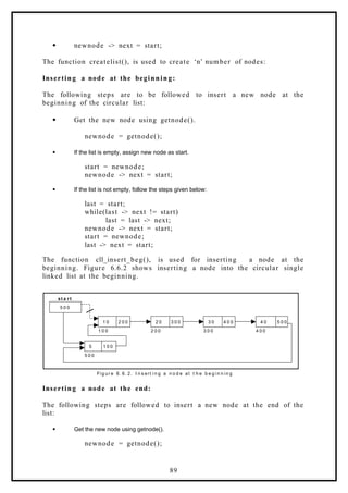
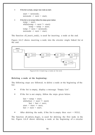
if(number[i] == data)
{
flag = 1;
break;
}
}
if(flag == 1)
printf("n Data found at location: %d", i+1);
else
printf("n Data not found ");
8

9. }
A Recursive program for linear search:
# include <stdio.h>
# include <conio.h>
void linear_search(int a[], int data, int position, int n)
{
int mid;
if(position < n)
{
if(a[position] == data)
printf("n Data Found at %d ", position);
else
linear_search(a, data, position + 1, n);
}
else
printf("n Data not found");
}
void main()
{
int a[25], i, n, data;
clrscr();
printf("n Enter the number of elements: ");
scanf("%d", &n);
printf("n Enter the elements: ");
for(i = 0; i < n; i++)
{
scanf("%d", &a[i]);
}
printf("n Enter the element to be seached: ");
scanf("%d", &data);
linear_search(a, data, 0, n);
getch();
}
BINARY SEARCH
If we have ‘n’ records which have been ordered by keys so that x1 < x2 < … < xn . When we are given a
element ‘x’, binary search is used to find the corresponding element from the list. In case ‘x’ is
present, we have to determine a value ‘j’ such that a[j] = x (successful search). If ‘x’ is not in the list
then j is to set to zero (un successful search).
In Binary search we jump into the middle of the file, where we find key a[mid], and compare ‘x’ with
a[mid]. If x = a[mid] then the desired record has been found. If x < a[mid] then ‘x’ must be in
that portion of the file that precedes a[mid]. Similarly, if a[mid] > x, then further search is only
necessary in that part of the file which follows a[mid]. If we use recursive procedure of finding the
middle key a[mid] of the un-searched portion of a file, then every un-successful comparison of ‘x’ with
a[mid] will eliminate roughly half the un-searched portion from consideration.
Since the array size is roughly halved after each comparison between ‘x’ and a[mid], and since an
array of length ‘n’ can be halved only about log2n times before reaching a trivial length, the worst case
complexity of Binary search is about log2n
Algorithm:
9

10. Let array a[n] of elements in increasing order, n  0, determine whether ‘x’ is present, and if so, set j
such that x = a[j] else return 0.
binsrch(a[], n, x)
{
low = 1; high = n;
while (low < high) do
{
mid =  (low + high)/2 
if (x < a[mid])
high = mid – 1;
else if (x > a[mid])
low = mid + 1;
else return mid;
}
return 0;
}
low and high are integer variables such that each time through the loop either ‘x’ is found or low is
increased by at least one or high is decreased by at least one. Thus we have two sequences of
integers approaching each other and eventually low will become greater than high causing
termination in a finite number of steps if ‘x’ is not present.
Example 1:
Let us illustrate binary search on the following 12 elements:
Index 1 2 3 4 5 6 7 8 9 10 11 12
Elements 4 7 8 9 16 20 24 38 39 45 54 77
If we are searching for x = 4: (This needs 3 comparisons)
low = 1, high = 12, mid = 13/2 = 6, check 20
low = 1, high = 5, mid = 6/2 = 3, check 8
low = 1, high = 2, mid = 3/2 = 1, check 4, found
If we are searching for x = 7: (This needs 4 comparisons)
low = 1, high = 12, mid = 13/2 = 6, check 20
low = 1, high = 5, mid = 6/2 = 3, check 8
low = 1, high = 2, mid = 3/2 = 1, check 4
low = 2, high = 2, mid = 4/2 = 2, check 7, found
If we are searching for x = 8: (This needs 2 comparisons)
low = 1, high = 12, mid = 13/2 = 6, check 20
low = 1, high = 5, mid = 6/2 = 3, check 8, found
If we are searching for x = 9: (This needs 3 comparisons)
low = 1, high = 12, mid = 13/2 = 6, check 20
low = 1, high = 5, mid = 6/2 = 3, check 8
low = 4, high = 5, mid = 9/2 = 4, check 9, found
If we are searching for x = 16: (This needs 4 comparisons)
low = 1, high = 12, mid = 13/2 = 6, check 20
low = 1, high = 5, mid = 6/2 = 3, check 8
low = 4, high = 5, mid = 9/2 = 4, check 9
low = 5, high = 5, mid = 10/2 = 5, check 16, found
If we are searching for x = 20: (This needs 1 comparison)
low = 1, high = 12, mid = 13/2 = 6, check 20, found
If we are searching for x = 24: (This needs 4 comparisons)
low = 1, high = 12, mid = 13/2 = 6, check 20
low = 7, high = 12, mid = 19/2 = 9, check 39
low = 7, high = 10, mid = 17/2 = 8, check 38
10

11. low = 7, high = 7, mid = 14/2 = 7, check 24, found
If we are searching for x = 38: (This needs 3 comparisons)
low = 1, high = 12, mid = 13/2 = 6, check 20
low = 7, high = 12, mid = 19/2 = 9, check 39
low = 7, high = 10, mid = 17/2 = 8, check 38, found
If we are searching for x = 39: (This needs 2 comparisons)
low = 1, high = 12, mid = 13/2 = 6, check 20
low = 7, high = 12, mid = 19/2 = 9, check 39, found
If we are searching for x = 45: (This needs 4 comparisons)
low = 1, high = 12, mid = 13/2 = 6, check 20
low = 7, high = 12, mid = 19/2 = 9, check 39
low = 10, high = 12, mid = 22/2 = 11, check 54
low = 10, high = 10, mid = 20/2 = 10, check 45, found
If we are searching for x = 54: (This needs 3 comparisons)
low = 1, high = 12, mid = 13/2 = 6, check 20
low = 7, high = 12, mid = 19/2 = 9, check 39
low = 10, high = 12, mid = 22/2 = 11, check 54, found
If we are searching for x = 77: (This needs 4 comparisons)
low = 1, high = 12, mid = 13/2 = 6, check 20
low = 7, high = 12, mid = 19/2 = 9, check 39
low = 10, high = 12, mid = 22/2 = 11, check 54
low = 12, high = 12, mid = 24/2 = 12, check 77, found
The number of comparisons necessary by search element:
20 – requires 1 comparison; 8 and 39 – requires 2 comparisons;
4, 9, 38, 54 – requires 3 comparisons; and 7, 16, 24, 45, 77 – requires 4 comparisons
Summing the comparisons, needed to find all twelve items and dividing by 12, yielding 37/12 or
approximately 3.08 comparisons per successful search on the average.
Example 2:
Let us illustrate binary search on the following 9 elements:
Index 1 2 3 4 5 6 7 8 9
Elements -15 -6 0 7 9 23 54 82 101
The number of comparisons required for searching different elements is as follows:
1. If we are searching for x = 101: (Number of comparisons = 4)
low high mid
1 9 5
6 9 7
8 9 8
9 9 9
found
2. Searching for x = 82: (Number of comparisons = 3)
low high mid
1 9 5
6 9 7
8 9 8
found
3. Searching for x = 42: (Number of comparisons = 4)
11

12. low high mid
1 9 5
6 9 7
5 6 5
6 6 6
7 6 not found
4. Searching for x = -14: (Number of comparisons = 3)
low high mid
1 9 5
4 4 2
1 1 1
2 1 not found
Continuing in this manner the number of element comparisons needed to find each of nine elements
is:
Index 1 2 3 4 5 6 7 8 9
Elements -15 -6 0 7 9 23 54 82 101
Comparisons 3 2 3 4 1 3 2 3 4
No element requires more than 4 comparisons to be found. Summing the comparisons needed to find
all nine items and dividing by 9, yielding 25/9 or approximately 2.77 comparisons per successful
search on the average.
There are ten possible ways that an un-successful search may terminate depending upon the value of
x.
If x < a(1), a(1) < x < a(2), a(2) < x < a(3), a(5) < x < a(6), a(6) < x < a(7) or a(7) < x < a(8) the
algorithm requires 3 element comparisons to determine that ‘x’ is not present. For all of the remaining
possibilities BINSRCH requires 4 element comparisons. Thus the average number of element
comparisons for an unsuccessful search is:
(3 + 3 + 3 + 4 + 4 + 3 + 3 + 3 + 4 + 4) / 10 = 34/10 = 3.4
Time Complexity:
The time complexity of binary search in a successful search is O(log n) and for an unsuccessful
search is O(log n).
A non-recursive program for binary search:
# include <stdio.h>
# include <conio.h>
main()
{
int number[25], n, data, i, flag = 0, low, high, mid;
clrscr();
printf("n Enter the number of elements: ");
scanf("%d", &n);
printf("n Enter the elements in ascending order: ");
for(i = 0; i < n; i++)
scanf("%d", &number[i]);
printf("n Enter the element to be searched: ");
scanf("%d", &data);
low = 0; high = n-1;
while(low <= high)
{
mid = (low + high)/2;
if(number[mid] == data)
12

13. {
flag = 1;
break;
}
else
{
if(data < number[mid])
high = mid - 1;
else
low = mid + 1;
}
}
if(flag == 1)
printf("n Data found at location: %d", mid + 1);
else
printf("n Data Not Found ");
}
A recursive program for binary search:
# include <stdio.h>
# include <conio.h>
void bin_search(int a[], int data, int low, int high)
{
int mid ;
if( low <= high)
{
mid = (low + high)/2;
if(a[mid] == data)
printf("n Element found at location: %d ", mid + 1);
else
{
if(data < a[mid])
bin_search(a, data, low, mid-1);
else
bin_search(a, data, mid+1, high);
}
}
else
printf("n Element not found");
}
void main()
{
int a[25], i, n, data;
clrscr();
printf("n Enter the number of elements: ");
scanf("%d", &n);
printf("n Enter the elements in ascending order: ");
for(i = 0; i < n; i++)
scanf("%d", &a[i]);
printf("n Enter the element to be searched: ");
scanf("%d", &data);
bin_search(a, data, 0, n-1);
getch();
}
Bubble Sort:
The bubble sort is easy to understand and program. The basic idea of bubble sort is to pass through
the file sequentially several times. In each pass, we compare each element in the file with its
13

14. successor i.e., X[i] with X[i+1] and interchange two element when they are not in proper order. We will
illustrate this sorting technique by taking a specific example. Bubble sort is also called as exchange
sort.
Consider the array x[n] which is stored in memory as shown below:
X[0] X[1] X[2] X[3] X[4] X[5]
33 44 22 11 66 55
Suppose we want our array to be stored in ascending order. Then we pass through the array 5 times
as described below:
Pass 1: (first element is compared with all other elements)
We compare X[i] and X[i+1] for i = 0, 1, 2, 3, and 4, and interchange X[i] and X[i+1] if X[i] > X[i+1]. The
process is shown below:
X[0] X[1] X[2] X[3] X[4] X[5] Remarks
33 44 22 11 66 55
22 44
11 44
44 66
55 66
33 22 11 44 55 66
The biggest number 66 is moved to (bubbled up) the right most position in the array.
Pass 2: (second element is compared)
We repeat the same process, but this time we don’t include X[5] into our comparisons. i.e., we
compare X[i] with X[i+1] for i=0, 1, 2, and 3 and interchange X[i] and X[i+1] if X[i] > X[i+1]. The
process is shown below:
X[0] X[1] X[2] X[3] X[4] Remarks
33 22 11 44 55
22 33
11 33
33 44
44 55
22 11 33 44 55
The second biggest number 55 is moved now to X[4].
Pass 3: (third element is compared)
We repeat the same process, but this time we leave both X[4] and X[5]. By doing this, we move the
third biggest number 44 to X[3].
X[0] X[1] X[2] X[3] Remarks
22 11 33 44
11 22
14

15. 22 33
33 44
11 22 33 44
Pass 4: (fourth element is compared)
We repeat the process leaving X[3], X[4], and X[5]. By doing this, we move the fourth biggest number
33 to X[2].
X[0] X[1] X[2] Remarks
11 22 33
11 22
22 33
Pass 5: (fifth element is compared)
We repeat the process leaving X[2], X[3], X[4], and X[5]. By doing this, we move the fifth biggest
number 22 to X[1]. At this time, we will have the smallest number 11 in X[0]. Thus, we see that we
can sort the array of size 6 in 5 passes.
For an array of size n, we required (n-1) passes.
Program for Bubble Sort:
#include <stdio.h>
#include <conio.h>
void bubblesort(int x[],int n)
{
int i, j, t;
for (i = 0; i < n; i++)
{
for (j = 0; j <n-i; j++)
{
if (x[j] > x[j+1])
{
t = x[j];
x[j] = x[j+1];
x[j+1] = t;
}
}
}
}
main()
{
int i, n, x[25];
clrscr();
printf("n Enter the number of elements: ");
scanf("%d",&n);
printf("n Enter Data:");
for(i = 0; i < n ; i++)
scanf("%d", &x[i]);
bubblesort(x,n);
printf ("nArray Elements after sorting: ");
for (i = 0; i < n; i++)
15

16. printf ("%5d", x[i]);
}
Time Complexity:
The bubble sort method of sorting an array of size n requires (n-1) passes and (n-1) comparisons on
each pass. Thus the total number of comparisons is (n-1) * (n-1) = n2
– 2n + 1, which is O(n2
).
Therefore bubble sort is very inefficient when there are more elements to sorting.
Selection Sort:
Now, you will learn another sorting technique, which is more efficient than bubble sort and the
insertion sort. This sort, as you will see, will not require no more than n-1 interchanges. The sort we
are talking about is selection sort.
Suppose x is an array of size n stored in memory. The selection sort algorithm first selects the
smallest element in the array x and place it at array position 0; then it selects the next smallest
element in the array x and place it at array position 1. It simply continues this procedure until it places
the biggest element in the last position of the array. We will now present to you an algorithm for
selection sort.
The array is passed through (n-1) times and the smallest element is placed in its respective position
in the array as detailed below:
Pass 1:
Find the location j of the smallest element in the array x [0], x[1], . . . . x[n-1], and then interchange x[j]
with x[0]. Then x[0] is sorted.
Pass 2:
Leave the first element and find the location j of the smallest element in the sub-array x[1], x[2], . . . .
x[n-1], and then interchange x[1] with x[j]. Then x[0], x[1] are sorted.
Pass 3:
Leave the first two elements and find the location j of the smallest element in the sub-array x[2], x[3], .
. . . x[n-1], and then interchange x[2] with x[j]. Then x[0], x[1], x[2] are sorted.
Pass (n-1):
Find the location j of the smaller of the elements x[n-2] and x[n-1], and then interchange x[j] and x[n-
2]. Then x[0], x[1], . . . . x[n-2] are sorted. Of course, during this pass x[n-1] will be the biggest
element and so the entire array is sorted.
Time Complexity:
In general we prefer selection sort in case where the insertion sort or the bubble sort requires
exclusive swapping. In spite of superiority of the selection sort over bubble sort and the insertion sort
(there is significant decrease in run time), its efficiency is also O(n2
) for n data items.
Example:
Let us consider the following example with 9 elements to analyze selection Sort:
1 2 3 4 5 6 7 8 9 Remarks
65 70 75 80 50 60 55 85 45 find the first smallest element
i j swap a[i] & a[j]
45 70 75 80 50 60 55 85 65 find the second smallest element
i j swap a[i] and a[j]
45 50 75 80 70 60 55 85 65 Find the third smallest element
i j swap a[i] and a[j]
16

17. 45 50 55 80 70 60 75 85 65 Find the fourth smallest element
i j swap a[i] and a[j]
45 50 55 60 70 80 75 85 65 Find the fifth smallest element
i j swap a[i] and a[j]
45 50 55 60 65 80 75 85 70 Find the sixth smallest element
i j swap a[i] and a[j]
45 50 55 60 65 70 75 85 80 Find the seventh smallest element
i j swap a[i] and a[j]
45 50 55 60 65 70 75 85 80 Find the eighth smallest element
i J swap a[i] and a[j]
45 50 55 60 65 70 75 80 85 The outer loop ends.
Non-recursive Program for selection sort:
# include<stdio.h>
# include<conio.h>
void selectionSort( int low, int high );
int a[25];
int main()
{
int num, i= 0;
clrscr();
printf( "Enter the number of elements: " );
scanf("%d", &num);
printf( "nEnter the elements:n" );
for(i=0; i < num; i++)
scanf( "%d", &a[i] );
selectionSort( 0, num - 1 );
printf( "nThe elements after sorting are: " );
for( i=0; i< num; i++ )
printf( "%d ", a[i] );
return 0;
}
void selectionSort( int low, int high )
{
int i=0, j=0, temp=0, minindex;
for( i=low; i <= high; i++ )
{
minindex = i;
for( j=i+1; j <= high; j++ )
if( a[j] < a[minindex] )
minindex = j;
temp = a[i];
a[i] = a[minindex];
a[minindex] = temp;
}
}
Recursive Program for selection sort:
#include <stdio.h>
17

18. #include<conio.h>
int x[6] = {77, 33, 44, 11, 66};
selectionSort(int);
main()
{
int i, n = 0;
clrscr();
printf (" Array Elements before sorting: ");
for (i=0; i<5; i++)
printf ("%d ", x[i]);
selectionSort(n); /* call selection sort */
printf ("n Array Elements after sorting: ");
for (i=0; i<5; i++)
printf ("%d ", x[i]);
}
selectionSort( int n)
{
int k, p, temp, min;
if (n== 4)
return (-1);
min = x[n];
p = n;
for (k = n+1; k<5; k++)
{
if (x[k] <min)
{
min = x[k];
p = k;
}
}
temp = x[n]; /* interchange x[n] and x[p] */
x[n] = x[p];
x[p] = temp;
n++ ;
selectionSort(n);
}
INSERTION SORT
The main idea behind the insertion sort is to insert the ith element
in its correct place in the ith pass. Suppose an array A with n elements
A[1], A[2],…A[N] is in memory. The insertion sort algorithm scans A
from A[1] to A[N], inserting each element A[K] into its proper position in
the previously sorted subarray A[1], A[2],..A[K-1].
Principle: In Insertion Sort algorithm, each element A[K] in the list is
compared with all the elements before it ( A[1] to A[K-1]). If any
element A[I] is found to be greater than A[K] then A[K] is inserted in
the place of A[I}. This process is repeated till all the elements are
sorted.
Algorith m:
18

19. Procedure INSERTIONSORT(A, N)
// A is the array containing the list of data items
// N is the number of data items in the list
Last ß N – 1
Repeat For Pass = 1 to Last Step 1
Repeat For I = 0 to Pass – 1 Step 1
If A[Pass] < A[I]
Then
Temp ß A[Pass]
Repeat For J = Pass -1 to I Step -1
A[J +1] ß A[J]
End Repeat
A[I] ß Temp
End If
End Repeat
End Repeat
End INSERTIONSORT
In Insertion Sort algorithm, Last is made to point to the last
element in the list and Pass is made to point to the second element in the
list. In every pass the Pass is incremented to point to the next element
and is continued till it reaches the last element. During each pass
A[Pass] is compared all elements before it. If A[Pass] is lesser than A[I]
in the list, then A[Pass] is inserted in position I. Finally, a sorted list is
obtained.
For performing the insertion operation, a variable temp is used to
safely store A[Pass] in it and then shift right elements starting from A[I]
to A[Pass- 1].
Example:
N = 10 à Number of elements in the list
L à Last
P à Pass
i = 0 i =1 i = 2 i = 3 i = 4 i = 5 i = 6 i = 7 i = 8 i = 9
42 23 74 11 65 58 94 36 99 87
P=1 A[P] < A[0] à Insert A[P] at 0 L=9
23 42 74 11 65 58 94 36 99 87
P=2 L=9
A[P] is greater than all elements before it. Hence No Change
19

20. 23 42 74 11 65 58 94 36 99 87
P=3 A[P] < A[0] à Insert A[P] at 0 L=9
11 23 42 74 65 58 94 36 99 87
P=4 L=9
A[P] < A[3] à Insert A[P] at 3
11 23 42 65 74 58 94 36 99 87
P=5 L=9
A[P] < A[3] à Insert A[P] at 3
11 23 42 58 65 74 94 36 99 87
P=6 L=9
A[P] is greater than all elements before it. Hence No Change
11 23 42 58 65 74 94 36 99 87
P=7 L=9
A[P] < A[2] à Insert A[P] at 2
11 23 36 42 58 65 74 94 99 87
P=8 L=9
A[P] is greater than all elements before it. Hence No Change
11 23 36 42 58 65 74 94 99 87
P, L=9
A[P] < A[7] à Insert A[P] at 7
Sorted List:
11 23 36 42 58 65 74 87 94 99
Progra m:
void array::sort()
{
int temp, last=count- 1;
for (int pass=1; pass< =last;pass + + )
{
for (int i=0; i<pass; i++)
{
20

21. if (a[pass]<a[i])
{
temp=a[pass];
for (int j=pass- 1;j> =i;j- -)
a[j+1]=a[j];
a[i]=temp;
}
}
}
}
In the sort function, the integer variable last is used to point to the
last element in the list. The first pass starts with the variable pass
pointing to the second element and continues till pass reaches the last
element. In each pass, a[pass] is compared with all the elements before
it and if a[pass] is lesser than a[i], then it is inserted in position i. Before
inserting it, the elements a[i] to a[pass- 1] are shifted right using a
temporary variable.
Advanta g e s:
1. Sorts the list faster when the list has less number of elements.
2. Efficient in cases where a new element has to be inserted into a
sorted list.
Disadvan t a g e s:
1. Very slow for large values of n.
2. Poor performance if the list is in almost reverse order.
21

22. Quick Sort
The quick sort was invented by Prof. C. A. R. Hoare in the early 1960’s. It was one of the first more
efficient sorting algorithms. It is an example of a class of algorithms that work by what is usually called
“divide and conquer”.
In essence, the quick sort algorithm partitions the original array by rearranging it into two groups. The
first group contains those elements less than some arbitrary chosen value taken from the set, and the
second group contains those elements greater than or equal to the chosen value.
The chosen value is known as the pivot element. Once the array has been rearranged in this way with
respect to the pivot, the very same partitioning is recursively applied to each of the two subsets.
When all the subsets have been partitioned and rearranged, the original array is sorted.
The function partition() makes use of two pointers up and down which are moved toward each other
in the following fashion:
1. Repeatedly increase the pointer up by one position until a[up] > =pivot.
2. Repeatedly decrease the pointer down by one position until a[down] <=pivot.
3. If down > up, interchange a[down] with a[up]
4. Repeat the steps 1, 2 and 3 till the ‘up’ pointer crosses the ‘down’ pointer. If ‘up’ pointer
crosses ‘down’ pointer, the position for pivot is found and place pivot element in ‘down’
pointer position.
The program uses a recursive function quicksort(). The algorithm of quick sort function sorts all
elements in an array ‘a’ between positions ‘low’ and ‘high’.
1. It terminates when the condition low >= high is satisfied. This condition will be satisfied
only when the array is completely sorted.
2. Here we choose the first element as the ‘pivot’. So, pivot = x[low]. Now it calls the
partition function to find the proper position j of the element x[low] i.e. pivot. Then we will
have two sub-arrays x[low], x[low+1], . . . . . . . x[j-1] and x[j+1], x[j+2], . . .x[high].
3. It calls itself recursively to sort the left sub-array x[low], x[low+1], . . . . . . . x[j-1] between
positions low and j-1 (where j is returned by the partition function).
4. It calls itself recursively to sort the right sub-array x[j+1], x[j+2], . . .x[high] between
positions j+1 and high.
Algorithm
Sorts the elements a[p], . . . . . ,a[q] which reside in the global array a[n] into ascending order. The a[n
+ 1] is considered to be defined and must be greater than all elements in a[n]; a[n + 1] = + 
quicksort (p, q)
{
if ( p < q ) then
{
call j = PARTITION(a, p, q+1); // j is the position of the partitioning element
call quicksort(p, j – 1);
call quicksort(j + 1 , q);
}
}
partition(a, m, p)
{
v = a[m]; up = m; down = p; // a[m] is the partition element
do
{
22

23. repeat
up = up + 1;
until (a[up] > v);
repeat
down = down – 1;
until (a[down] < v);
if (up < down) then call interchange(a, up, down);
} while (up > down);
a[m] = a[down];
a[down] = v;
return (down);
}
interchange(a, up, down)
{
p = a[up];
a[up] = a[down];
a[down] = p;
}
Time complexity:
There are several choices for choosing the ‘pivot’ element through which we can improve the
efficiency of quick sort. For example, one may choose the ‘pivot’ element as median or mean or
middle element. Also, a non-recursive method could be developed for execution efficiency. When
these improvements are made, experiments indicate the fact that the total number of comparisons for
quick sort is of O(n log n).
Example:
Select first element as the pivot element. Move ‘up’ pointer from left to right in search of an element
larger than pivot. Move the ‘down’ pointer from right to left in search of an element smaller than pivot.
If such elements are found, the elements are swapped. This process continues till the ‘up’ pointer
crosses the ‘down’ pointer. If ‘up’ pointer crosses ‘down’ pointer, the position for pivot is found and
interchange pivot and element at ‘down’ position.
Let us consider the following example with 13 elements to analyze quick sort:
1
2 3 4 5 6 7 8 9 10 11 12 13 Remarks
38 08 16 06 79 57 24 56 02 58 04 70 45
pivot up
dow
n
swap up
& down
04 79
up
dow
n
swap up
& down
02 57
dow
n
up
(24 08 16 06 04 02) 38 (56 57 58 79 70 45)
swap
pivot &
down
pivot
dow
n
swap
pivot &
down
(02 08 16 06 04) 24
pivot,
down
up swap
pivot &
23

24. down
02 (08 16 06 04)
pivot up
dow
n
swap up
& down
04 16
dow
n
Up
(06 04) 08
(16)
swap
pivot &
down
pivot
,
dow
n
up
(04) 06
swap
pivot &
down
04
pivot
,
dow
n
16
pivot
,
dow
n
(02 04 06 08 16 24) 38
(56 57 58 79 70 45)
pivot up
dow
n
swap up
& down
45 57
dow
n
up
(45) 56 (58 79 70 57)
swap
pivot &
down
45
pivot
,
dow
n
swap
pivot &
down
(58
pivot
79
up
70
57)
dow
n
swap up
& down
57 79
dow
n
up
(57) 58 (70 79)
swap
pivot &
down
57
pivot
,
dow
n
(70 79)
pivot
,
dow
n
up
swap
pivot &
down
70
79
pivot
,
dow
24

25. n
(45 56 57 58 70 79)
02 04 06 08 16 24 38 45 56 57 58 70 79
Program for Quick Sort (Recursive version):
# include<stdio.h>
# include<conio.h>
void quicksort(int, int);
int partition(int, int);
void interchange(int, int);
int array[25];
int main()
{
int num, i = 0;
clrscr();
printf( "Enter the number of elements: " );
scanf( "%d", &num);
printf( "Enter the elements: " );
for(i=0; i < num; i++)
scanf( "%d", &array[i] );
quicksort(0, num -1);
printf( "nThe elements after sorting are: " );
for(i=0; i < num; i++)
printf("%d ", array[i]);
return 0;
}
void quicksort(int low, int high)
{
int pivotpos;
if( low < high )
{
pivotpos = partition(low, high + 1);
quicksort(low, pivotpos - 1);
quicksort(pivotpos + 1, high);
}
}
int partition(int low, int high)
{
int pivot = array[low];
int up = low, down = high;
do
{
do
up = up + 1;
while(array[up] < pivot );
do
down = down - 1;
while(array[down] > pivot);
if(up < down)
interchange(up, down);
}while(up < down);
25

26. array[low] = array[down];
array[down] = pivot;
return down;
}
void interchange(int i, int j)
{
int temp;
temp = array[i];
array[i] = array[j];
array[j] = temp;
}
Heap and Heap Sort
Heap is a data structure, which permits one to insert elements into a set and also to find the largest
element efficiently. A data structure, which provides these two operations, is called a priority queue.
Max and Min Heap data structures:
A max heap is an almost complete binary tree such that the value of each node is greater than or
equal to those in its children.
M a x h e a p
M i n h e a p
9 5
8 5
7 5 2 5
4 5
1 5
3 5
4 5
5 5
1 5
6 5 3 5
2 5
7 5
5 5 6 5 8 5 9 5
A min heap is an almost complete binary tree such that the value of each node is less than or equal to
those in its children.
Representation of Heap Tree:
Since heap is a complete binary tree, a heap tree can be efficiently represented using one
dimensional array. This provides a very convenient way of figuring out where children belong to.
 The root of the tree is in location 1.
 The left child of an element stored at location i can be found in location 2*i.
 The right child of an element stored at location i can be found in location 2*i+1.
 The parent of an element stored at location i can be found at location floor(i/2).
The elements of the array can be thought of as lying in a tree structure. A heap tree represented
using a single array looks as follows:
X[1] X[2] X[3] X[4] X[5] X[6] X[7] X[8]
65 45 60 40 25 50 55 30
26

27. 2 5 5 5
6 0
5 0
6 5
4 5
3 0
4 0
x[ 1]
x[ 3]
x[ 7]
x[ 6]
x[ 2]
x[ 5]
x[ 4]
x[ 8] He a p T r e e
Operations on heap tree:
The major operations required to be performed on a heap tree:
1. Insertion,
2. Deletion and
3. Merging.
Insertion into a heap tree:
This operation is used to insert a node into an existing heap tree satisfying the properties of heap
tree. Using repeated insertions of data, starting from an empty heap tree, one can build up a heap
tree.
Let us consider the heap (max) tree. The principle of insertion is that, first we have to adjoin the data
in the complete binary tree. Next, we have to compare it with the data in its parent; if the value is
greater than that at parent then interchange the values. This will continue between two nodes on path
from the newly inserted node to the root node till we get a parent whose value is greater than its child
or we reached the root.
For illustration, 35 is added as the right child of 80. Its value is compared with its parent’s value, and
to be a max heap, parent’s value greater than child’s value is satisfied, hence interchange as well as
further comparisons are no more required.
As another illustration, let us consider the case of insertion 90 into the resultant heap tree. First, 90
will be added as left child of 40, when 90 is compared with 40 it requires interchange. Next, 90 is
compared with 80, another interchange takes place. Now, our process stops here, as 90 is now in
root node. The path on which these comparisons and interchanges have taken places are shown by
dashed line.
The algorithm Max_heap_insert to insert a data into a max heap tree is as follows:
Max_heap_insert (a, n)
{
//inserts the value in a[n] into the heap which is stored at a[1] to a[n-1]
integer i, n;
i = n;
item = a[n] ;
while ( (i > 1) and (a[  i/2  ] < item ) do
{
a[i] = a[  i/2  ] ; // move the parent down
i =  i/2  ;
}
a[i] = item ;
return true ;
}
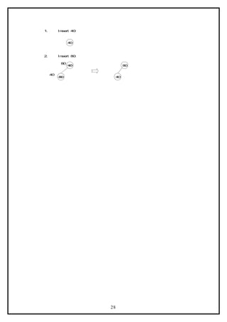
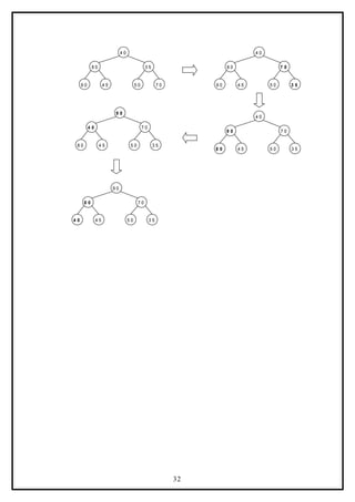
Example:
Form a heap by using the above algorithm for the given data 40, 80, 35, 90, 45, 50, 70.
27

28. 40
40
80
80
40
1
. Inse
rt 40
:
2
. Inse
rt 80
:
80
40
28

29. 9 0
8 0
4 0
5 0
9 0
3 5
9 0
9 0
8 0
4 5
4 0 3 5
5 0
8 0
3 5
4 0
8 0
4 . I n s e r t 9 0 :
3 . I n s e r t 3 5 :
5 . I n s e r t 4 5 :
6 . I n s e r t 5 0 :
4 5
4 0 4 5
9 0
7 . I n s e r t 7 0 :
9 0
4 5 3 5
7 0
4 5 3 5
3 5
8 0
4 0
4 0
8 0
5 0
7 0
5 0
5 0
3 5
7 0
5 0
8 0
4 0 3 5
4 0
9 0
8 0 3 5
4 0
9 0
9 0
8 0
adjust (a, i, n)
// The complete binary trees with roots a(2*i) and a(2*i + 1) are combined with a(i) to form a single
heap, 1 < i < n. No node has an address greater than n or less than 1. //
{
j = 2 *i ;
item = a[i] ;
while (j < n) do
29

30. {
if ((j < n) and (a (j) < a (j + 1)) then j ß j + 1;
// compare left and right child and let j be the larger child
if (item > a (j)) then break;
// a position for item is found
else a[  j / 2  ] = a[j] // move the larger child up a level
j = 2 * j;
}
a [  j / 2  ] = item;
}
Here the root node is 99. The last node is 26, it is in the level 3. So, 99 is replaced by 26 and this
node with data 26 is removed from the tree. Next 26 at root node is compared with its two child 45
and 63. As 63 is greater, they are interchanged. Now, 26 is compared with its children, namely, 57
and 42, as 57 is greater, so they are interchanged. Now, 26 appears as the leave node, hence re-
heap is completed.
9 9
4 5 6 3
3 5 5 7 4 2
2 9
2 7 1 2 2 4 2 6
6 3
4 5 5 7
3 5 2 6 4 2
2 9
2 7 1 2 2 4
2 6 6 3
2 6
5 7
2 6
De l e t i n g t h e n o d e w it h d at a 9 9 Af t er De l e t i o n of n o d e w it h d at a 9 9
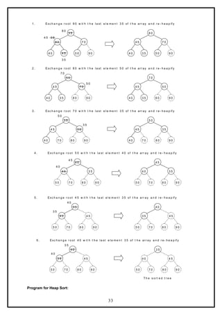
HEAP SORT:
A heap sort algorithm works by first organizing the data to be sorted into a special type of binary tree
called a heap. Any kind of data can be sorted either in ascending order or in descending order using
heap tree. It does this with the following steps:
1. Build a heap tree with the given set of data.
2. a. Remove the top most item (the largest) and replace it with the last
element in the heap.
b. Re-heapify the complete binary tree.
c. Place the deleted node in the output.
3. Continue step 2 until the heap tree is empty.
Algorithm:
This algorithm sorts the elements a[n]. Heap sort rearranges them in-place in non-decreasing order.
First transform the elements into a heap.
heapsort(a, n)
{
heapify(a, n);
for i = n to 2 by – 1 do
{
temp = a[I];
a[i] = a[1];
a[1] = t;
adjust (a, 1, i – 1);
}
30

31. }
heapify (a, n)
//Readjust the elements in a[n] to form a heap.
{
for i ß  n/2  to 1 by – 1 do adjust (a, i, n);
}
adjust (a, i, n)
// The complete binary trees with roots a(2*i) and a(2*i + 1) are combined with a(i) to form a single
heap, 1 < i < n. No node has an address greater than n or less than 1. //
{
j = 2 *i ;
item = a[i] ;
while (j < n) do
{
if ((j < n) and (a (j) < a (j + 1)) then j ß j + 1;
// compare left and right child and let j be the larger child
if (item > a (j)) then break;
// a position for item is found
else a[  j / 2  ] = a[j] // move the larger child up a level
j = 2 * j;
}
a [  j / 2  ] = item;
}
Time Complexity:
Each ‘n’ insertion operations takes O(log k), where ‘k’ is the number of elements in the heap at the
time.
Likewise, each of the ‘n’ remove operations also runs in time O(log k), where ‘k’ is the number of
elements in the heap at the time.
Since we always have k ≤n, each such operation runs in O(log n) time in the worst case.
Thus, for ‘n’ elements it takes O(n log n) time, so the priority queue sorting algorithm runs in O(n log
n) time when we use a heap to implement the priority queue.
Example 1:
Form a heap from the set of elements (40, 80, 35, 90, 45, 50, 70) and sort the data using heap sort.
Solution:
First form a heap tree from the given set of data and then sort by repeated deletion operation:
31

32. 4 0
3 5
8 0
7 0
9 0 4 5 5 0
4 0
7 0
8 0
3 5
9 0 4 5 5 0
4 0
8 0
9 0
5 0 3 5
7 0
9 0
8 0
4 0
4 5
7 0
3 5
3 5
3 5
7 0
5 0 3 5
7 0
9 0
4 0
8 0
4 5
4 5 5 0 3 5
32

33. 3 5
7 0
9 0
8 0
5 0
4 5
4 0
8 0
3 5
4 5
3 5
8 0
7 0
9 0
4 5
5 0
3 5
4 0
9 0
4 5 7 0
5 0
8 0
3 5
4 0
7 0
5 0
8 0
3 5
4 0
4 5
7 0
9 0
5 0
3 5
5 0
4 5
3 5
4 0 7 0 8 0 9 0
5 0
8 0
3 5
7 0
4 0
4 5
5 0
9 0
1. Exc h a n g e r o ot 9 0 w it h t h e l a st e l e m e n t 3 5 of t h e arr ay a n d r e - h e a p if y
2. Exc h a n g e r o ot 8 0 w it h t h e l a st e l e m e n t 5 0 of t h e arr ay a n d r e - h e a p if y
3. Exc h a n g e r o ot 7 0 w it h t h e l a st e l e m e n t 3 5 of t h e arr ay a n d r e- h e a p if y
4 0
3 5
9 0
4 5
8 0
7 0
5 0
4 5
4 0
4 5
3 5
9 0
4 0
8 0
7 0
5 0
9 0
4 0 4 5
3 5
8 0
7 0
5 0
4 0
8 0
7 0
5 0
3 5
4 0
9 0
4 5
4 0
4 5
3 5
5 0 7 0 8 0 9 0
3 5
8 0
4 5
7 0
5 0
4 0
3 5
9 0
3 5
4 0
4. Exc h a n g e r o ot 5 0 w it h t h e l a st e l e m e n t 4 0 of t h e arr ay a n d r e - h e a p if y
5. Exc h a n g e r o ot 4 5 w it h t h e l a st e l e m e n t 3 5 of t h e arr ay a n d r e - h e a p if y
6. Exc h a n g e r o ot 4 0 w it h t h e l a st e l e m e n t 3 5 of t h e arr ay a n d r e - h e a p if y
T h e s ort e d t r e e
Program for Heap Sort:
33

34. # include <stdio.h>
# include <conio.h>
void adjust(int i, int n, int a[])
{
int j, item;
j = 2 * i;
item = a[i];
while(j <= n)
{
if((j < n) && (a[j] < a[j+1]))
j++;
if(item >= a[j])
break;
else
{
a[j/2] = a[j];
j = 2*j;
}
}
a[j/2] = item;
}
void heapify(int n, int a[])
{
int i;
for(i = n/2; i > 0; i--)
adjust(i, n, a);
}
void heapsort(int n,int a[])
{
int temp, i;
heapify(n, a);
for(i = n; i > 0; i--)
{
temp = a[i];
a[i] = a[1];
a[1] = temp;
adjust(1, i - 1, a);
}
}
void main()
{
int i, n, a[20];
clrscr();
printf("n How many element you want: ");
scanf("%d",&n);
printf("Enter %d elements: ",n);
for (i=1;i<=n;i++)
scanf("%d", &a[i]);
heapsort(n, a);
printf("n The sorted elements are: n");
for (i=1;i<=n;i++)
printf("%5d",a[i]);
getch();
}
MERGE SORT
34

35. Principle: The given list is divided into two roughly equal parts called
the left and the right subfiles. These subfiles are sorted using the
algorithm recursively and then the two subfiles are merged together to
obtain the sorted file.
Given a sequence of n elements A[1], ….A[N], the general idea is to
imagine them split into two sets A[1],…A[N/2] and A[(N/2) + 1],…A[N].
Each set is individually sorted, and the resulting sorted sequences are
merged to produce a single sorted sequence of N elements. Thus this
sorting method follows Divide and Conquer strategy.
Algorith m:
Procedure MERGE(A, low, mid, high)
// A is the array containing the list of data items
I ß low, J ß mid+1, K ß low
While I mid and J high
≤ ≤
If A[I] < A[J]
Then
Temp[K] ß A[I]
I ß I + 1
K ß K+1
Else
Temp[K] ß A[J]
J ß J + 1
K ß K + 1
End If
End While
If I > mid
Then
While J high
≤
Temp[K] ß A[J]
K ß K + 1
J ß J + 1
End While
Else
While I mid
≤
Temp[K] ß A[I]
K ß K + 1
I ß I + 1
End While
End If
Repeat for K = low to high step 1
A[K] ß Temp[K]
End Repeat
End MERGE
35

36. Procedure MERGESORT(A, low, high)
// A is the array containing the list of data items
If low < high
Then
mid ß (low + high)/2
MERGESORT(low, high)
MERGESORT(mid + 1, high)
MERGE(low, mid, high)
End If
End MERGESORT
The first algorithm MERGE can be applied on two sorted lists to
merge them. Initially, the index variable I points to low and J points to
mid + 1. A[I] is compared with A[J] and if A[I] found to be lesser than
A[J] then A[I] is stored in a temporary array and I is incremented
otherwise A[J] is stored in the temporary array and J is incremented.
This comparison is continued until either I crosses mid or J crosses high.
If I crosses the mid first then that implies that all the elements in first list
is accommodated in the temporary array and hence the remaining
elements in the second list can be put into the temporary array as it is. If
J crosses the high first then the remaining elements of first list is put as
it is in the temporary array. After this process we get a single sorted list.
Since this method merges 2 lists at a time, this is called 2-way merge
sort.
In the MERGESORT algorithm, the given unsorted list is first split
into N number of lists, each list consisting of only 1 element. Then the
MERGE algorithm is applied for first 2 lists to get a single sorted list.
Then the same thing is done on the next two lists and so on. This process
is continued till a single sorted list is obtained.
Example:
Let L à low, Mà mid, H à high
i = 0 i =1 i = 2 i = 3 i = 4 i = 5 i = 6 i = 7 i = 8 i = 9
42 23 74 11 65 58 94 36 99 87
U M H
In each pass the mid value is calculated and based on that the list is split
into two. This is done recursively and at last N number of lists each
having only one element is produced as shown.
36

37. Now merging operation is called on first two lists to produce a single
sorted list, then the same thing is done on the next two lists and so on.
Finally a single sorted list is obtained.
Progra m:
void array::sort(int low, int high)
{
int mid;
if (low<high)
{
mid=(low+high)/2;
sort(low,mid);
sort(mid+1, high);
merge(low, mid, high);
}
}
void array::merge(int low, int mid, int high)
{
int i=low, j=mid+1, k=low, temp[MAX];
while (i<=mid && j<=high)
if (a[i]<a[j])
temp[k+ +] = a[i + + ];
else
temp[k+ +] = a[j + + ];
if (i>mid)
while (j<=high)
temp[k+ +] = a[j + + ];
else
while (i<=mid)
temp[k+ +] = a[i + + ];
37

38. for (k=low; k<=high; k++)
a[k]=temp[k];
}
Advanta g e s:
1. Very useful for sorting bigger lists.
2. Applicable for external sorting also.
Disadvan t a g e s:
1. Needs a temporary array every time, for storing the new sorted
list.
shell Sort
The shell sort , sometimes called the “diminishing increment sort,”
improves on the insertion sort by breaking the original list into a number
of smaller sublists, each of which is sorted using an insertion sort. The
unique way that these sublists are chosen is the key to the shell sort.
Instead of breaking the list into sublists of contiguous items, the shell
sort uses an increment i, sometimes called the gap , to create a sublist by
choosing all items that are i items apart.
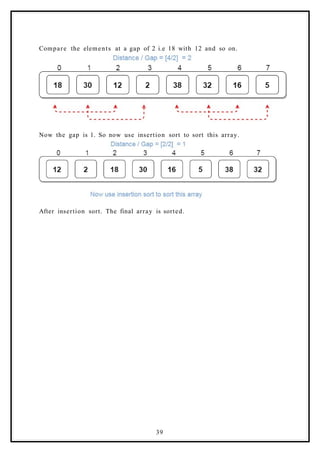
Example of shell Sort : Use Shell sort for the following array : 18, 32, 12,
5, 38, 30, 16, 2
Compare the elements at a gap of 4. i.e 18 with 38 and so on and swap if
first number is greater than second.
38

39. Compare the elements at a gap of 2 i.e 18 with 12 and so on.
Now the gap is 1. So now use insertion sort to sort this array.
After insertion sort. The final array is sorted.
39

40. UNIT- II
STACKS
The data structures seen so far, allows insertion and deletion of
elements at any place. But sometimes it is required to permit the
addition and deletion of elements only at one end that is either at the
beginning or at the end.
Stacks: A stack is a data structure in which addition of new element
or deletion of an existing element always takes place at the same end.
This end is often known as top of stack. When an item is added to a
stack, the operation is called push, and when an item is removed from
the stack the operation is called pop. Stack is also called as Last- In-
First- Out (LIFO) list.
Operation s on Stack:
There are two possible operations done on a stack. They are pop
and push operation.
 Push: Allows adding an element at the top of the stack.
 Pop: Allows removing an element from the top of the stack.
The Stack can be implemented using both arrays and linked lists.
When dynamic memory allocation is preferred we go for linked lists to
implement the stacks.
ARRAY IMPLEMENTATION OF THE STACK
Push operation:
If the elements are added continuously to the stack using the push
operation then the stack grows at one end. Initially when the stack is
empty the top = -1. The top is a variable which indicates the position of
the topmost element in the stack.
40

41. PUSH(x)
If top = MAX – 1
Then
Print “Stack is full”
Return
Else
Top = top + 1
A[top] = x
End if
End PUSH( )
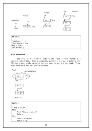
Pop operation:
On deletion of elements the stack shrinks at the same end, as the
elements at the top get removed.
POP( )
If top = -1
Then
Print “Stack is empty”
Return
Else
Item = A[top]
A[Top] = 0
Top = top – 1
Return item
End if
End POP( )
If arrays are used for implementing the stacks, it would be very
easy to manage the stacks. However, the problem with an array is that
we are required to declare the size of the array before using it in a
program. This means the size of the stack should be fixed. We can
declare the array with a maximum size large enough to manage a stack.
As result, the stack can grow or shrink within the space reserved for it.
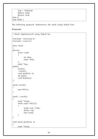
The following program implements the stack using array.
Progra m:
41

42. // Stack and various operations on it
#include <iostream.h >
#include <conio.h>
const int MAX=20;
class stack
{
private:
int a[MAX];
int top;
public:
stack();
void push(int x);
int pop();
void display();
};
stack::stack()
{
top=- 1;
}
void stack::push(int x)
{
if (top= = MAX- 1)
{
cout< <"nStack is full!";
return;
}
else
{
top+ +;
a[top]=x;
}
}
int stack::pop()
{
if (top= =- 1)
{
cout< <"nStack is empty!";
return NULL;
}
else
{
int item=a[top];
top- -;
return item;
42

43. }
}
void stack::display()
{
int temp=top;
while (temp!=- 1)
cout< <"n"< < a[temp- -];
}
void main()
{
clrscr();
stack s;
int n;
s.push(10);
s.push(20);
s.push(30);
s.push(40);
s.display();
n=s.pop();
cout< <"nPopped item:"< < n;
n=s.pop();
cout< <"nPopped item:"< < n;
s.display();
getch();
}
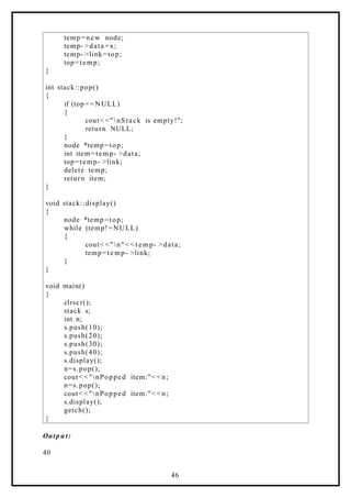
Output:
40
30
20
10
Popped item:40
Popped item:30
20
10
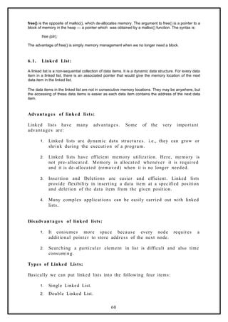
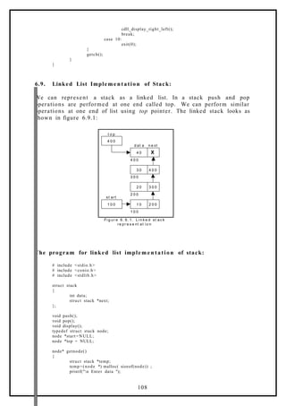
LINKED LIST IMPLEMENTATION OF STACK
Initially, when the stack is empty, top points to NULL. When an
element is added using the push operation, top is made to point to the
latest element whichever is added.
Push operation:
Create a temporary node and store the value of x in the data part
of the node. Now make link part of temp point to Top and then top point
to Temp. That will make the new node as the topmost element in the
stack.
43

44. PUSH(x)
Info(temp) = x
Link(temp) = top
Top = temp
End PUSH( )
Pop operation
The data in the topmost node of the stack is first stored in a
variable called item. Then a temporary pointer is created to point to top.
The top is now safely moved to the next node below it in the stack. Temp
node is deleted and the item is returned.
POP( )
If Top = NULL
Then
Print “Stack is empty”
Return
Else
Item = info(top)
Temp = top
44

45. Top = link(top)
Delete temp
Return item
End if
End POP( )
The following program implements the stack using linked lists.
Progra m:
// Stack implemented using linked list
#include <iostream.h >
#include <conio.h>
class stack
{
private:
struct node
{
int data;
node *link;
};
node *top;
public:
stack();
~stack();
void push(int x);
int pop();
void display();
};
stack::stack()
{
top=NULL;
}
stack::~stack()
{
node *temp;
while (top!=NULL)
{
temp=top- >link;
delete top;
top=temp;
}
}
void stack::push(int x)
{
node *temp;
45

46. temp=new node;
temp- >data =x;
temp- >link=top;
top=temp;
}
int stack::pop()
{
if (top= = NULL)
{
cout< <"nStack is empty!";
return NULL;
}
node *temp=top;
int item=temp- >data;
top=temp- >link;
delete temp;
return item;
}
void stack::display()
{
node *temp=top;
while (temp!=NULL)
{
cout< <"n"< < t e m p- >data;
temp=temp- >link;
}
}
void main()
{
clrscr();
stack s;
int n;
s.push(10);
s.push(20);
s.push(30);
s.push(40);
s.display();
n=s.pop();
cout< <"nPopped item:"< < n;
n=s.pop();
cout< <"nPopped item:"< < n;
s.display();
getch();
}
Output:
40
46

47. 30
20
10
Popped item:40
Popped item:30
20
10
APPLICATION OF STACKS
Conversion of Infix Expression to Postfix Expression
The stacks are frequently used in evaluation of arithmetic
expressions. An arithmetic expression consists of operands and
operators. The operands can be numeric values or numeric variables.
The operators used in an arithmetic expression represent the operations
like addition, subtraction, multiplication, division and exponentiation.
The arithmetic expression expressed in its normal form is said to
be Infix notation, as shown:
A + B
The above expression in prefix form would be represented as follows:
+ AB
The same expression in postfix form would be represented as follows:
AB +
Hence the given expression in infix form is first converted to postfix form
and then evaluated to get the results.
The function to convert an expression from infix to postfix consists
following steps:
1. Every character of the expression string is scanned in a while loop
until the end of the expression is reached.
2. Following steps are performed depending on the type of character
scanned.
(a) If the character scanned happens to be a space then that
character is skipped.
(b) If the character scanned is a digit or an alphabet, it is added
to the target string pointed to by t.
(c) If the character scanned is a closing parenthesis then it is
added to the stack by calling push( ) function.
(d) If the character scanned happens to be an operator, then
firstly, the topmost element from the stack is retrieved.
Through a while loop, the priorities of the character scanned
47

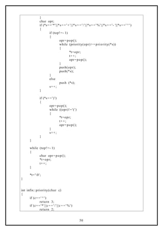
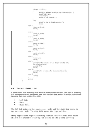
48. and the character popped ‘opr’ are compared. Then
following steps are performed as per the precedence rule.
i. If ‘opr’ has higher or same priority as the character
scanned, then opr is added to the target string.
ii. If opr has lower precedence than the character
scanned, then the loop is terminated. Opr is pushed
back to the stack. Then, the character scanned is also
added to the stack.
(e) If the character scanned happens to be an opening
parenthesis, then the operators present in the stack are
retrieved through a loop. The loop continues till it does not
encounter a closing parenthesis. The operators popped, are
added to the target string pointed to by t.
2. Now the string pointed by t is the required postfix expression.
Progra m:
// Program to convert an Infix form to Postfix form
#include <iostream.h >
#include <string.h>
#include <ctype.h>
#include <conio.h>
const int MAX=50;
class infix
{
private:
char target[MAX], stack[MAX];
char *s, *t;
int top;
public:
infix();
void push(char c);
char pop();
void convert(char *str);
int priority (char c);
void show();
};
infix::infix()
{
top=- 1;
strcpy(target,"");
strcpy(stack,"");
t=target;
s="";
48

49. }
void infix::push(char c)
{
if (top= = MAX- 1)
cout< <"nStack is fulln!";
else
{
top+ +;
stack[top]=c;
}
}
char infix::pop()
{
if (top= =- 1)
{
cout< <"nStack is emptyn";
return -1;
}
else
{
char item=stack[top];
top- -;
return item;
}
}
void infix::convert(char *str)
{
s=str;
while(*s!='0')
{
if (*s==' '||*s= ='t')
{
s++;
continue;
}
if (isdigit(*s) || isalpha(*s))
{
while(isdigit(*s) || isalpha(*s))
{
*t=*s;
s++;
t++;
}
}
if (*s=='(')
{
push(*s);
s++;
49

50. }
char opr;
if (*s=='*'||*s= = ' + ' ||*s = = '/'||*s= = '%'||*s = = '- '||*s= =' ^ ')
{
if (top!=- 1)
{
opr=pop();
while (priority(opr)> = p riority(*s))
{
*t=opr;
t++;
opr=pop();
}
push(opr);
push(*s);
}
else
push (*s);
s++;
}
if (*s==')')
{
opr=pop();
while ((opr)!='(')
{
*t=opr;
t++;
opr=pop();
}
s++;
}
}
while (top!=- 1)
{
char opr=pop();
*t=opr;
t++;
}
*t='0';
}
int infix::priority(char c)
{
if (c==' ^ ')
return 3;
if (c=='*'||c= = '/'||c = = ' %')
return 2;
50

51. else
{
if (c==' +'||c = = '- ')
return 1;
else
return 0;
}
}
void infix::show()
{
cout< < t a rget;
}
void main()
{
clrscr();
char expr[MAX], *res[MAX];
infix q;
cout< <"nEnter an expression in infix form: ";
cin> > expr;
q.convert(expr);
cout< <"nThe postfix expression is: ";
q.show();
getch();
}
Output:
Enter an expression in infix form: 5^2- 5
Stack is empty
The postfix expression is: 52^5-
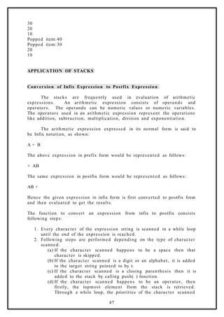
Evaluation of Expression entered in postfix form
The program takes the input expression in postfix form. This
expression is scanned character by character. If the character scanned
is an operand, then first it is converted to a digit form and then it is
pushed onto the stack. If the character scanned is a blank space, then it
is skipped. If the character scanned is an operator, then the top two
elements from the stack are retrieved. An arithmetic operation is
performed between the two operands. The type of arithmetic operation
depends on the operator scanned from the string s. The result is then
pushed back onto the stack. These steps are repeated as long as the
string s is not exhausted. Finally the value in the stack is the required
result and is shown to the user.
51

52. Progra m:
// Program to evaluate an expression entered in postfix form
#include <iostream.h >
#include <stdlib.h>
#include <math.h >
#include <ctype.h>
#include <conio.h>
const int MAX=50;
class postfix
{
private:
int stack[MAX];
int top, n;
char *s;
public:
postfix();
void push(int item);
int pop();
void calculate(char *str);
void show();
};
postfix::postfix()
{
top=- 1;
}
void postfix::push(int item)
{
if (top= = MAX- 1)
cout< < e ndl < < "Stack is full";
else
{
top+ +;
stack[top]=item;
}
}
int postfix::pop()
{
if (top= =- 1)
{
cout< < e ndl < < "Stack is empty";
52

53. return NULL;
}
int data=stack[top];
top- -;
return data;
}
void postfix::calculate(char *str)
{
s=str;
int n1, n2, n3;
while (*s)
{
if (*s==' '||*s= ='t')
{
s++;
continue;
}
if (isdigit(*s))
{
n=*s- '0';
push(n);
}
else
{
n1=pop();
n2=pop();
switch(*s)
{
case '+':
n3=n2 + n 1;
break;
case '-':
n3=n2- n1;
break;
case '/':
n3=n2/n1;
break;
case '*':
n3=n2*n1;
break;
case '%':
n3=n2%n1;
break;
case '^':
n3=pow(n2, n1);
break;
default:
cout< <"Unknown operator";
exit(1);
}
push(n3);
53

54. }
s++;
}
}
void postfix::show()
{
n=pop();
cout< <"Result is: "<<n;
}
void main()
{
clrscr();
char expr[MAX];
cout << "nEnter postfix expression to be evaluated : ";
cin> > expr;
postfix q ;
q.calculate(expr);
q.show();
getch();
}
Output:
Enter postfix expression to be evaluated : 53^5-
Result is: 120
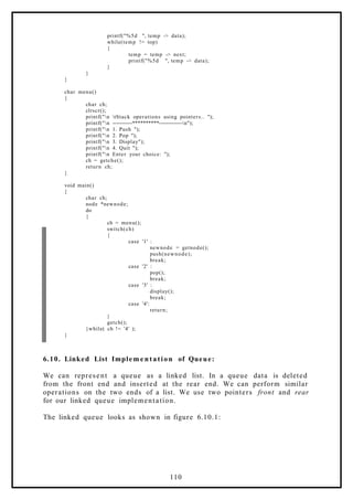
QUEUE
Queue: Queue is a linear data structure that permits insertion of new
element at one end and deletion of an element at the other end. The
end at which the deletion of an element take place is called front, and
the end at which insertion of a new element can take place is called
rear. The deletion or insertion of elements can take place only at the
front or rear end of the list respectively.
The first element that gets added into the queue is the first one to
get removed from the list. Hence, queue is also referred to as First- In-
First- Out list (FIFO). Queues can be represented using both arrays as
well as linked lists.
ARRAY IMPLEMENTATION OF QUEUE
If queue is implemented using arrays, the size of the array should
be fixed maximum allowing the queue to expand or shrink.
Operation s on a Queue
There are two common operations one in a queue. They are
addition of an element to the queue and deletion of an element from the
queue. Two variables front and rear are used to point to the ends of the
queue. The front points to the front end of the queue where deletion
takes place and rear points to the rear end of the queue, where the
54

55. addition of elements takes place. Initially, when the queue is full, the
front and rear is equal to -1.
Add(x)
An element can be added to the queue only at the rear end of the
queue. Before adding an element in the queue, it is checked whether
queue is full. If the queue is full, then addition cannot take place.
Otherwise, the element is added to the end of the list at the rear side.
ADDQ(x)
If rear = MAX – 1
Then
Print “Queue is full”
Return
Else
Rear = rear + 1
A[rear] = x
If front = -1
Then
Front = 0
End if
End if
End ADDQ( )
Del( )
The del( ) operation deletes the element from the front of the
queue. Before deleting and element, it is checked if the queue is empty.
If not the element pointed by front is deleted from the queue and front is
now made to point to the next element in the queue.
DELQ( )
If front = -1
Then
Print “Queue is Empty”
Return
55

56. Else
Item = A[front]
A[front] = 0
If front = rear
Then
Front = rear = -1
Else
Front = front + 1
End if
Return item
End if
End DELQ( )
Progra m:
// Queues and various operations on it – Using arrays
#include <iostream.h >
#include <conio.h>
const int MAX=10;
class queue
{
private:
int a[MAX], front, rear;
public:
queue();
void addq(int x);
int delq();
void display();
};
queue::queue()
{
front=rear =- 1;
}
void queue::addq(int x)
{
if (rear= = MAX- 1)
{
cout< <"Queue is full!";
return;
}
rear+ + ;
a[rear]=x;
if (front= =- 1)
front=0;
}
int queue::delq()
56

57. {
if (front= =- 1)
{
cout< <"Queue is empty!";
return NULL;
}
int item=a[front];
a[front]=0;
if (front= = r e a r)
front=rear =- 1;
else
front+ +;
return item;
}
void queue::display()
{
if (front= =- 1)
return;
for (int i=front; i<=rear; i++)
cout< < a[i]< <"t";
}
void main()
{
clrscr();
queue q;
q.addq(50);
q.addq(40);
q.addq(90);
q.display();
cout< < e ndl;
int i=q.delq();
cout< < e ndl;
cout< <i < < " deleted!";
cout< < e ndl;
q.display();
i=q.delq();
cout< < e ndl;
cout< <i < < " deleted!";
cout< < e ndl;
i=q.delq();
cout< <i < < " deleted!";
cout< < e ndl;
i=q.delq();
getch();
}
Output:
57

58. 50 40 90
50 deleted!
40 90
40 deleted!
90 deleted!
Queue is empty!
58

59. Unit 3
LINKED LISTS
Linked lists and arrays are similar since they both store collections of
data. One way to think about linked lists is to look at how arrays work
and think about alternate approaches.
Array is the most common data structure used to store collections of elements. Arrays are convenient
to declare and provide the easy syntax to access any element by its index number. Once the array is
set up, access to any element is convenient and fast.
The disadvantag e s of arrays are:
 The size of the array is fixed. Most often this size is specified at
compile time. This makes the programmers to allocate arrays,
which seems "large enough" than required.
 Inserting new elements at the front is potentially expensive
because existing elements need to be shifted over to make
room.
 Deleting an element from an array is not possible.
Linked lists have their own strengths and weaknesses, but they happen to be strong where arrays are
weak. Generally array's allocates the memory for all its elements in one block whereas linked lists use
an entirely different strategy.
Linked lists allocate memory for each element separately and only when
necessary.
Here is a quick review of the terminology and rules of pointers. The
linked list code will depend on the following functions:
malloc() is a system function which allocates a block of memory in the
"heap" and returns a pointer to the new block. The prototype of malloc()
and other heap functions are in stdlib.h. malloc() returns NULL if it
cannot fulfill the request. It is defined by:
void *malloc (number_of_bytes)
Since a void * is returned the C standard states that this pointer can be converted to any type. For
example,
char *cp;
cp = (char *) malloc (100);
Attempts to get 100 bytes and assigns the starting address to cp. We can also use the sizeof()
function to specify the number of bytes. For example,
int *ip;
ip = (int *) malloc (100*sizeof(int));
59

60. free() is the opposite of malloc(), which de-allocates memory. The argument to free() is a pointer to a
block of memory in the heap — a pointer which was obtained by a malloc() function. The syntax is:
free (ptr);
The advantage of free() is simply memory management when we no longer need a block.
6.1. Linked List:
A linked list is a non-sequential collection of data items. It is a dynamic data structure. For every data
item in a linked list, there is an associated pointer that would give the memory location of the next
data item in the linked list.
The data items in the linked list are not in consecutive memory locations. They may be anywhere, but
the accessing of these data items is easier as each data item contains the address of the next data
item.
Advantage s of linked lists:
Linked lists have many advantages. Some of the very important
advantages are:
1. Linked lists are dynamic data structures. i.e., they can grow or
shrink during the execution of a program.
2. Linked lists have efficient memory utilization. Here, memory is
not pre- allocated. Memory is allocated whenever it is required
and it is de- allocated (removed) when it is no longer needed.
3. Insertion and Deletions are easier and efficient. Linked lists
provide flexibility in inserting a data item at a specified position
and deletion of the data item from the given position.
4. Many complex applications can be easily carried out with linked
lists.
Disadvantag e s of linked lists:
1. It consumes more space because every node requires a
additional pointer to store address of the next node.
2. Searching a particular element in list is difficult and also time
consuming.
Types of Linked Lists:
Basically we can put linked lists into the following four items:
1. Single Linked List.
2. Double Linked List.
60

61. 3. Circular Linked List.
4. Circular Double Linked List.
A single linked list is one in which all nodes are linked together in some
sequential manner. Hence, it is also called as linear linked list.
A double linked list is one in which all nodes are linked together by
multiple links which helps in accessing both the successor node (next
node) and predecessor node (previous node) from any arbitrary node
within the list. Therefore each node in a double linked list has two link
fields (pointers) to point to the left node (previous) and the right node
(next). This helps to traverse in forward direction and backward
direction.
A circular linked list is one, which has no beginning and no end. A single
linked list can be made a circular linked list by simply storing address of
the very first node in the link field of the last node.
A circular double linked list is one, which has both the successor pointer
and predecessor pointer in the circular manner.
Comparison betwee n array and linked list:
ARRAY LINKED LIST
Size of an array is fixed Size of a list is not fixed
Memory is allocated from stack Memory is allocated from heap
It is necessary to specify the
number of elements during
declaration (i.e., during compile
time).
It is not necessary to specify the
number of elements during
declaration (i.e., memory is
allocated during run time).
It occupies less memory than a
linked list for the same number
of elements.
It occupies more memory.
Inserting new elements at the
front is potentially expensive
because existing elements need
to be shifted over to make room.
Inserting a new element at any
position can be carried out easily.
Deleting an element from an
array is not possible.
Deleting an element is possible.
Applications of linked list:
1. Linked lists are used to represent and manipulate polynomial.
Polynomials are expression containing terms with non zero
coefficient and exponents. For example:
P(x) = a 0 Xn + a 1 Xn-1 + …… + a n-1 X + a n
61

62. 2. Represent very large numbers and operations of the large number
such as addition, multiplication and division.
3. Linked lists are to implement stack, queue, trees and graphs.
4. Implement the symbol table in compiler construction
6.2. Single Linked List:
A linked list allocates space for each element separately in its own block of memory called a "node".
The list gets an overall structure by using pointers to connect all its nodes together like the links in a
chain.
Each node contains two fields; a "data" field to store whatever element,
and a "next" field which is a pointer used to link to the next node.
Each node is allocated in the heap using malloc(), so the node memory
continues to exist until it is explicitly de- allocated using free(). The front
of the list is a pointer to the “start” node. A single linked list is shown in
figure 6.2.1.
1 0 0
1 0 2 0 0 2 0 3 0 0 3 0 4 0 0 4 0 X
1 0 0 2 0 0 3 0 0 4 0 0
st a rt
Fi g ur e 6. 2. 1. S i n g l e Li n k e d Li st
H E A P
S T A C K
T h e n e xt f i e l d of
t h e l a st n o d e i s
N ULL.
T h e st art
p o i nt er
h o l d s t h e
a d dr e s s of
t h e f ir st
n o d e of t h e
l i st .
Eac h n o d e
st or e s t h e d at a.
St or e s t h e n e xt
n o d e a d dr e s s.
The beginning of the linked list is stored in a "start " pointer which points
to the first node. The first node contains a pointer to the second node.
The second node contains a pointer to the third node, ... and so on. The
last node in the list has its next field set to NULL to mark the end of the
list. Code can access any node in the list by starting at the start and
following the next pointers.
The start pointer is an ordinary local pointer variable, so it is drawn
separately on the left top to show that it is in the stack. The list nodes
are drawn on the right to show that they are allocated in the heap.
Impleme n tation of Single Linked List:
62

63. Before writing the code to build the above list, we need to create a start
node , used to create and access other nodes in the linked list. The
following structure definition will do (see figure 6.2.2):
 Creating a structure with one data item and a next pointer,
which will be pointing to next node of the list. This is called as
self-referential structure.
 Initialise the start pointer to be NULL.
NULL
st a rt
Fi g ur e 6. 2. 2. St r uc t ur e d ef i n it i o n, s i n g l e l i n k n o d e a n d e m p t y l i st
E m p t y list :
st r uct s lin k list
{
int d at a;
st r uct s lin k list * n e x t ;
} ;
t y p e d ef st r uct s lin k list no d e;
no d e * st a rt = NULL;
d at a n e xt
n o d e :
The basic operations in a single linked list are:
 Creation.
 Insertion.
 Deletion.
 Traversing.
Creating a node for Single Linked List:
Creating a singly linked list starts with creating a node. Sufficient memory has to be allocated for
creating a node. The information is stored in the memory, allocated by using the malloc() function.
The function getnode(), is used for creating a node, after allocating memory for the structure of type
node, the information for the item (i.e., data) has to be read from the user, set next field to NULL and
finally returns the address of the node. Figure 6.2.3 illustrates the creation of a node for single linked
list.
no d e* g et no d e( )
{
no d e* n e w no d e;
n e w no d e = ( no d e * ) m a llo c( s iz eo f( no d e) ) ;
p r int f( " n Ent e r d at a: " ) ;
sca nf( " % d " , & n e w no d e - > d at a) ;
n e w no d e - > n e x t = NULL;
r et u r n n e w no d e;
}
1 0 X
n e w n o d e
1 0 0
Fi g ur e 6. 2. 3. n e w n o d e w it h a v a l u e of 1 0
Creating a Singly Linked List with ‘n’ number of nodes:
The following steps are to be followed to create ‘n’ number of nodes:
63

64.  Get the new node using getnode().
newnode = getnode();
 If the list is empty, assign new node as start.
start = newnode;
 If the list is not empty, follow the steps given below:
 The next field of the new node is made to point the first
node (i.e. start node) in the list by assigning the address of
the first node.
 The start pointer is made to point the new node by
assigning the address of the new node.
 Repeat the above steps ‘n’ times.
Figure 6.2.4 shows 4 items in a single linked list stored at different
locations in memory.
1 0 0
1 0 2 0 0 2 0 3 0 0 3 0 4 0 0 4 0 X
1 0 0 2 0 0 3 0 0 4 0 0
st a rt
Fi g ur e 6. 2. 4. S i n g l e Li n k e d Li st w it h 4 n o d e s
The function createlist(), is used to create ‘n’ number of nodes:
v o id c r e at e list ( int n)
{
int i;
no d e * n e w no d e;
no d e * t e m p ;
fo r( i = 0 ; i < n ; i+ + )
{
n e w no d e = g et no d e( ) ;
if( st a rt = = N ULL)
{
st a rt = n e w no d e;
}
e ls e
{
t e m p = st a rt ;
w h ile( t e m p - > n e x t ! = NULL)
t e m p = t e m p - > n e x t ;
t e m p - > n e x t = n e w no d e;
}
}
}
64

65. Insertion of a Node:
One of the most primitive operations that can be done in a singly linked list is the insertion of a node.
Memory is to be allocated for the new node (in a similar way that is done while creating a list) before
reading the data. The new node will contain empty data field and empty next field. The data field of
the new node is then stored with the information read from the user. The next field of the new node is
assigned to NULL. The new node can then be inserted at three different places namely:
 Inserting a node at the beginning.
 Inserting a node at the end.
 Inserting a node at intermediate position.
Inserting a node at the beginnin g:
The following steps are to be followed to insert a new node at the
beginning of the list:
 Get the new node using getnode().
newnode = getnode();
 If the list is empty then start = newnode.
 If the list is not empty, follow the steps given below:
newnode -> next = start;
start = newnode;
The function insert_at_beg(), is used for inserting a node at the
beginning
Figure 6.2.5 shows inserting a node into the single linked list at the
beginning.
65

66. 5 0 0
1 0 2 0 0 2 0 3 0 0 3 0 4 0 0 4 0 X
1 0 0 2 0 0 3 0 0 4 0 0
st a rt
Fi g ur e 6. 2. 5. I n s ert i n g a n o d e at t h e b e g i n n i n g
5 1 0 0
5 0 0
Inserting a node at the end:
The following steps are followed to insert a new node at the end of the
list:
 Get the new node using getnode()
newnode = getnode();
 If the list is empty then start = newnode.
 If the list is not empty follow the steps given below:
temp = start;
while(temp -> next != NULL)
temp = temp -> next;
temp -> next = newnode;
The function insert_at_end(), is used for inserting a node at the end.
Figure 6.2.6 shows inserting a node into the single linked list at the end.
1 0 0
1 0 2 0 0 2 0 3 0 0 3 0 4 0 0 4 0 5 0 0
1 0 0 2 0 0 3 0 0 4 0 0
st a rt
Fi g ur e 6. 2. 6. I n s ert i n g a n o d e at t h e e n d.
5 0 X
5 0 0
Inserting a node at intermediate position:
The following steps are followed, to insert a new node in an intermediate position in the list:
 Get the new node using getnode().
newnode = getnode();
66

67.  Ensure that the specified position is in between first node and
last node. If not, specified position is invalid. This is done by
countnode() function.
 Store the starting address (which is in start pointer) in temp and
prev pointers. Then traverse the temp pointer upto the specified
position followed by prev pointer.
 After reaching the specified position, follow the steps given
below:
prev -> next = newnode;
newnode -> next = temp;
 Let the intermediate position be 3.
The function insert_at_mid(), is used for inserting a node in the
intermediate position.
Figure 6.2.7 shows inserting a node into the single linked list at a specified intermediate position other
than beginning and end.
1 0 0
1 0 2 0 0 2 0 5 0 0 3 0 4 0 0 4 0 X
1 0 0 2 0 0 3 0 0 4 0 0
st a rt
Fi g ur e 6. 2. 7. I n s ert i n g a n o d e at a n i nt er m e d i a t e p o s it i o n.
5 0 3 0 0
5 0 0
t e m p
pr ev
n e w n o d e
Deletion of a node:
Another primitive operation that can be done in a singly linked list is the
deletion of a node. Memory is to be released for the node to be deleted. A
node can be deleted from the list from three different places namely.
 Deleting a node at the beginning.
 Deleting a node at the end.
 Deleting a node at intermediate position.
Deleting a node at the beginnin g:
67

68. The following steps are followed, to delete a node at the beginning of the
list:
 If list is empty then display ‘Empty List’ message.
 If the list is not empty, follow the steps given below:
temp = start;
start = start -> next;
free(temp);
The function delete_at_beg(), is used for deleting the first node in the list.
Figure 6.2.8 shows deleting a node at the beginning of a single linked list.
2 00
1 0 20 0 2 0 3 00 30 4 0 0 4 0 X
1 0 0 20 0 3 00 40 0
st a rt
Fig ur e 6. 2. 8. Delet in g a no d e at t h e b eg in ning.
t e mp
Deleting a node at the end:
The following steps are followed to delete a node at the end of the list:
 If list is empty then display ‘Empty List’ message.
 If the list is not empty, follow the steps given below:
temp = prev = start;
while(temp -> next != NULL)
{
prev = temp;
temp = temp -> next;
}
prev -> next = NULL;
free(temp);
The function delete_at_last(), is used for deleting the last node in the list.
Figure 6.2.9 shows deleting a node at the end of a single linked list.
68

69. 1 0 0
1 0 2 0 0 2 0 3 0 0 3 0 X 4 0 X
1 0 0 2 0 0 3 0 0 4 0 0
st a rt
Fi g ur e 6. 2. 9. De l e t i n g a n o d e at t h e e n d.
Deleting a node at Intermediate position:
The following steps are followed, to delete a node from an intermediate
position in the list (List must contain more than two node).
 If list is empty then display ‘Empty List’ message
 If the list is not empty, follow the steps given below.
if(pos > 1 && pos < nodectr)
{
temp = prev = start;
ctr = 1;
while(ctr < pos)
{
prev = temp;
temp = temp -> next;
ctr+ +;
}
prev -> next = temp -> next;
free(temp);
printf("n node deleted..");
}
The function delete_at_mid(), is used for deleting the intermediate node
in the list.
Figure 6.2.10 shows deleting a node at a specified intermediate position other than beginning and
end from a single linked list.
1 0 0
1 0 3 0 0 2 0 3 0 0 3 0 4 0 0 4 0 X
1 0 0 2 0 0 3 0 0 4 0 0
st a rt
Fig ur e 6. 2. 1 0. De le t i n g a n o d e at a n i nt er me d ia t e p o s it io n.
Traversal and displaying a list (Left to Right):
69

70. To display the information, you have to traverse (move) a linked list,
node by node from the first node, until the end of the list is reached.
Traversing a list involves the following steps:
 Assign the address of start pointer to a temp pointer.
 Display the information from the data field of each node.
The function traverse () is used for traversing and displaying the
information stored in the list from left to right.
v o id t r a v e rs e( )
{
no d e * t e m p ;
t e m p = st a rt ;
p r int f( " n Th e co nt e nt s o f List ( Left t o Rig h t ) : n" ) ;
if( st a rt = = NULL )
p r int f( " n Em p t y List " ) ;
e ls e
w h ile( t e m p ! = NULL)
{
p r int f( " % d - > " , t e m p - > d at a) ;
t e m p = t e m p - > n e x t ;
}
p r int f( " X" ) ;
}
Alternatively there is another way to traverse and display the
information. That is in reverse order. The function rev_traverse(), is used
for traversing and displaying the information stored in the list from right
to left.
v o id r e v _ t r a v e rs e( no d e * st )
{
if( st = = NULL)
{
r et u r n;
}
e ls e
{
r e v _ t r a v e rs e( st - > n e x t ) ;
p r int f( " % d - > " , st - > d at a) ;
}
}
Counting the Number of Nodes:
The following code will count the number of nodes exist in the list using
recursion .
70

71. int co u nt no d e( no d e * st )
{
if( st = = NULL)
r et u r n 0 ;
e ls e
r et u r n( 1 + co u nt no d e( st - > n e x t ) ) ;
}
6.3.A Complete Source Code for the Implementation of Single Linked List:
# include <stdio.h>
# include <conio.h>
# include <stdlib.h>
struct slinklist
{
int data;
struct slinklist *next;
};
typedef struct slinklist node;
node *start = NULL;
int menu()
{
int ch;
clrscr();
printf("n 1.Create a list ");
printf("n- -------------------------");
printf("n 2.Insert a node at beginning ");
printf("n 3.Insert a node at end");
printf("n 4.Insert a node at middle");
printf("n- -------------------------");
printf("n 5.Delete a node from beginning");
printf("n 6.Delete a node from Last");
printf("n 7.Delete a node from Middle");
printf("n- -------------------------");
printf("n 8.Traverse the list (Left to Right)");
printf("n 9.Traverse the list (Right to Left)");
printf("n- -------------------------");
printf("n 10. Count nodes ");
printf("n 11. Exit ");
printf("nn Enter your choice: ");
scanf("%d",&ch);
return ch;
}
node* getnode()
{
node * newnode;
newnode = (node *) malloc(sizeof(node));
printf("n Enter data: ");
scanf("%d", &newnode -> data);
newnode -> next = NULL;
return newnode;
}
int countnode(node *ptr)
{
int count=0;
while(ptr != NULL)
{
count+ +;
ptr = ptr -> next;
71

72. }
return (count);
}
void createlist(int n)
{
int i;
node *newnode;
node *temp;
for(i = 0; i < n; i++)
{
newnode = getnode();
if(start == NULL)
{
start = newnode;
}
else
{
temp = start;
while(temp -> next != NULL)
temp = temp -> next;
temp -> next = newnode;
}
}
}
void traverse()
{
node *temp;
temp = start;
printf("n The contents of List (Left to Right): n");
if(start == NULL)
{
printf("n Empty List");
return;
}
else
while(temp != NULL)
{
printf("%d- ->", temp -> data);
temp = temp -> next;
}
printf(" X ");
}
void rev_traverse(node *start)
{
if(start == NULL)
{
return;
}
else
{
rev_traverse(start -> next);
printf("%d -->", start -> data);
}
}
void insert_at_beg()
{
node *newnode;
newnode = getnode();
if(start == NULL)
{
start = newnode;
}
else
{
newnode -> next = start;
72

73. start = newnode;
}
}
void insert_at_end()
{
node *newnode, *temp;
newnode = getnode();
if(start == NULL)
{
start = newnode;
}
else
{
temp = start;
while(temp -> next != NULL)
temp = temp -> next;
temp -> next = newnode;
}
}
void insert_at_mid()
{
node *newnode, *temp, *prev;
int pos, nodectr, ctr = 1;
newnode = getnode();
printf("n Enter the position: ");
scanf("%d", &pos);
nodectr = countnode(start);
if(pos > 1 && pos < nodectr)
{
temp = prev = start;
while(ctr < pos)
{
prev = temp;
temp = temp -> next;
ctr+ +;
}
prev -> next = newnode;
newnode -> next = temp;
}
else
{
printf("position %d is not a middle position", pos);
}
}
void delete_at_beg()
{
node *temp;
if(start == NULL)
{
printf("n No nodes are exist..");
return ;
}
else
{
temp = start;
start = temp -> next;
free(temp);
printf("n Node deleted ");
}
}
void delete_at_last()
{
node *temp, *prev;
if(start == NULL)
{
73

74. printf("n Empty List..");
return ;
}
else
{
temp = start;
prev = start;
while(temp -> next != NULL)
{
prev = temp;
temp = temp -> next;
}
prev -> next = NULL;
free(temp);
printf("n Node deleted ");
}
}
void delete_at_mid()
{
int ctr = 1, pos, nodectr;
node *temp, *prev;
if(start == NULL)
{
printf("n Empty List..");
return ;
}
else
{
printf("n Enter position of node to delete: ");
scanf("%d", &pos);
nodectr = countnode(start);
if(pos > nodectr)
{
printf("nThis node doesnot exist");
}
if(pos > 1 && pos < nodectr)
{
temp = prev = start;
while(ctr < pos)
{
prev = temp;
temp = temp -> next;
ctr ++;
}
prev -> next = temp -> next;
free(temp);
printf("n Node deleted..");
}
else
{
printf("n Invalid position..");
getch();
}
}
}
void main(void)
{
int ch, n;
clrscr();
while(1)
{
ch = menu();
switch(ch)
{
case 1:
74

75. if(start == NULL)
{
printf("n Number of nodes you want to create: ");
scanf("%d", &n);
createlist(n);
printf("n List created..");
}
else
printf("n List is already created..");
break;
case 2:
insert_at_beg();
break;
case 3:
insert_at_end();
break;
case 4:
insert_at_mid();
break;
case 5:
delete_at_beg();
break;
case 6:
delete_at_last();
break;
case 7:
delete_at_mid();
break;
case 8:
traverse();
break;
case 9:
printf("n The contents of List (Right to Left): n");
rev_traverse(start);
printf(" X ");
break;
case 10:
printf("n No of nodes : %d ", countnode(start));
break;
case 11 :
exit(0);
}
getch();
}
}
6.4. Double Linked List:
A double linked list is a two-way list in which all nodes will have two links. This helps in accessing
both successor node and predecessor node from the given node position. It provides bi-directional
traversing. Each node contains three fields:
 Left link.
 Data.
 Right link.
The left link points to the predecessor node and the right link points to
the successor node. The data field stores the required data.
Many applications require searching forward and backward thru nodes
of a list. For example searching for a name in a telephone directory
75

76. would need forward and backward scanning thru a region of the whole
list.
The basic operations in a double linked list are:
 Creation.
 Insertion.
 Deletion.
 Traversing.
A double linked list is shown in figure 6.3.1.
1 0 0
X 1 0 2 0 0 2 0 0 3 0 X
1 0 0 2 0 0 3 0 0
st a rt
Fi g ur e 6. 3. 1. Do u b l e Li n k e d Li st
H E A P
S T A C K
T h e r i g ht f i e l d of
t h e l a st n o d e i s
N ULL.
T h e st art
p o i nt er
h o l d s t h e
a d dr e s s of
t h e f ir st
n o d e of t h e
l i st .
St or e s t h e d at a. St or e s t h e n e xt
n o d e a d dr e s s.
1 0 0 2 0 3 0 0
St or e s t h e
pr ev i o u s n o d e
a d dr e s s.
The beginning of the double linked list is stored in a "start " pointer
which points to the first node. The first node’s left link and last node’s
right link is set to NULL.
The following code gives the structure definition:
NULL
st a rt
Fi g ur e 6. 4. 1. St r uc t ur e d ef i n it i o n, d o u b l e l i n k n o d e a n d e m p t y l i st
E m p t y list :
st r uct d lin k list
{
st r uct d lin k list * left ;
int d at a;
st r uct d lin k list * r ig ht ;
} ;
t y p e d ef st r uct d lin k list no d e;
no d e * st a rt = NULL;
l ef t d at a r ig ht
n o d e :
Creating a node for Double Linked List:
Creating a double linked list starts with creating a node. Sufficient
memory has to be allocated for creating a node. The information is
stored in the memory, allocated by using the malloc() function. The
function getnode(), is used for creating a node, after allocating memory
for the structure of type node, the information for the item (i.e., data) has
to be read from the user and set left field to NULL and right field also set
to NULL (see figure 6.2.2).
76

77. no d e* g et no d e( )
{
no d e* n e w no d e;
n e w no d e = ( no d e * ) m a llo c( s iz eo f( no d e) ) ;
p r int f( " n Ent e r d at a: " ) ;
sca nf( " % d " , & n e w no d e - > d at a) ;
n e w no d e - > left = NULL;
n e w no d e - > r ig ht = NULL;
r et u r n n e w no d e;
}
X 1 0 X
n e w n o d e
1 0 0
Fi g ur e 6. 4. 2. n e w n o d e w it h a v a lu e of 1 0
Creating a Double Linked List with ‘n’ number of nodes:
The following steps are to be followed to create ‘n’ number of nodes:
 Get the new node using getnode().
newnode =getnode();
 If the list is empty then start = newnode.
 If the list is not empty, follow the steps given below:
 The left field of the new node is made to point the
previous node.
 The previous nodes right field must be assigned with
address of the new node.
 Repeat the above steps ‘n’ times.
The function createlist(), is used to create ‘n’ number of nodes:
v o id c r e at e list ( int n)
{
int i;
no d e * n e w no d e;
no d e * t e m p ;
fo r( i = 0 ; i < n; i+ + )
{
n e w no d e = g et no d e( ) ;
if( st a rt = = NU LL)
{
st a rt = n e w no d e;
}
e ls e
{
t e m p = st a rt ;
w h ile( t e m p - > r ig ht )
t e m p = t e m p - > r ig ht ;
t e m p - > r ig ht = n e w no d e;
n e w no d e - > left = t e m p ;
}
}
}
77

78. Figure 6.4.3 shows 3 items in a double linked list stored at different
locations.
1 0 0
X 1 0 2 0 0 2 0 0 3 0 X
1 0 0 2 0 0 3 0 0
st a rt
Fi g ur e 6. 4. 3. Do u b l e Li n k e d Li st w it h 3 n o d e s
1 0 0 2 0 3 0 0
Inserting a node at the beginnin g:
The following steps are to be followed to insert a new node at the
beginning of the list:
 Get the new node using getnode().
newnode = g etnode();
 If the list is empty then start = newnode.
 If the list is not empty, follow the steps given below:
newnode -> right = start;
start -> left = newnode;
start = newnode;
The function dbl_insert_beg(), is used for inserting a node at the
beginning. Figure 6.4.4 shows inserting a node into the double linked list
at the beginning.
4 0 0
4 0 0 1 0 2 0 0 2 0 0 3 0 X
1 0 0 2 0 0 3 0 0
st a rt
Fi g ur e 6. 4. 4. I n s ert i n g a n o d e at t h e b e g i n n in g
1 0 0 2 0 3 0 0
X 4 0 1 0 0
4 0 0
Inserting a node at the end:
The following steps are followed to insert a new node at the end of the
list:
 Get the new node using getnode()
78

79. newnode=getnode();
 If the list is empty then start = newnode.
 If the list is not empty follow the steps given below:
temp = start;
while(temp -> right != NULL)
temp = temp -> right;
temp -> right = newnode;
newnode -> left = temp;
The function dbl_insert_end(), is used for inserting a node at the end.
Figure 6.4.5 shows inserting a node into the double linked list at the end.
1 0 0
X 1 0 2 0 0 2 0 0 3 0 4 0 0
1 0 0 2 0 0 3 0 0
st a rt
Fi g ur e 6. 4. 5. I n s ert i n g a n o d e at t h e e n d
1 0 0 2 0 3 0 0
3 0 0 4 0 X
4 0 0
Inserting a node at an intermediate position:
The following steps are followed, to insert a new node in an intermediate position in the list:
 Get the new node using getnode().
newnode = g etnode();
 Ensure that the specified position is in between first node and
last node. If not, specified position is invalid. This is done by
countnode() function.
 Store the starting address (which is in start pointer) in temp and
prev pointers. Then traverse the temp pointer upto the specified
position followed by prev pointer.
 After reaching the specified position, follow the steps given
below:
newnode -> left = temp;
newnode -> right = temp -> right;
temp -> right -> left = newnode;
temp -> right = newnode;
79

80. The function dbl_insert_mid(), is used for inserting a node in the
intermediate position. Figure 6.4.6 shows inserting a node into the
double linked list at a specified intermediate position other than
beginning and end.
1 0 0
X 1 0 4 0 0
4 0 0 2 0 3 0 0
1 0 0
4 0 0
2 0 0
st a rt
Fi g ur e 6. 4. 6. I n s ert i n g a n o d e at a n i nt er me d i a t e p o s it i o n
1 0 0 4 0 2 0 0
2 0 0 3 0 X
3 0 0
Deleting a node at the beginnin g:
The following steps are followed, to delete a node at the beginning of the
list:
 If list is empty then display ‘Empty List’ message.
 If the list is not empty, follow the steps given below:
temp = start;
start = start -> right;
start -> left = NULL;
free(temp);
The function dbl_delete_beg(), is used for deleting the first node in the
list. Figure 6.4.6 shows deleting a node at the beginning of a double
linked list.
2 0 0
X 1 0 2 0 0 2 0 0 3 0 X
1 0 0 2 0 0 3 0 0
st a rt
Fi g ur e 6. 4. 6. De l e t i n g a n o d e at b e g i n n i n g
X 2 0 3 0 0
Deleting a node at the end:
The following steps are followed to delete a node at the end of the list:
 If list is empty then display ‘Empty List’ message
 If the list is not empty, follow the steps given below:
temp = start;
80

81. while(temp -> right != NULL)
{
temp = temp -> right;
}
temp -> left -> right = NULL;
free(temp);
The function dbl_delete_last(), is used for deleting the last node in the
list. Figure 6.4.7 shows deleting a node at the end of a double linked list.
1 0 0
X 1 0 2 0 0 2 0 0 3 0 X
1 0 0 2 0 0 3 0 0
st a rt
Fi g ur e 6. 4. 7. De l e t i n g a n o d e at t h e e n d
1 0 0 2 0 X
Deleting a node at Intermediate position:
The following steps are followed, to delete a node from an intermediate
position in the list (List must contain more than two nodes).
 If list is empty then display ‘Empty List’ message.
 If the list is not empty, follow the steps given below:
 Get the position of the node to delete.
 Ensure that the specified position is in between first node
and last node. If not, specified position is invalid.
 Then perform the following steps:
if(pos > 1 && pos < nodectr)
{
temp = start;
i = 1;
while(i < pos)
{
temp = temp -> right;
i++;
}
temp -> right -> left = temp -> left;
temp -> left -> right = temp -> right;
free(temp);
printf("n node deleted..");
}
81

82. The function delete_at_mid(), is used for deleting the intermediate node in the list. Figure 6.4.8 shows
deleting a node at a specified intermediate position other than beginning and end from a double
linked list.
1 0 0
X 1 0 3 0 0 1 0 0 3 0 X
1 0 0 2 0 0 3 0 0
st a rt
Fi g ur e 6. 4. 8 De l e t i n g a n o d e at a n i nt er m e d i a t e p o s it i o n
1 0 0 2 0 3 0 0
Traversal and displaying a list (Left to Right):
To display the information, you have to traverse the list, node by node
from the first node, until the end of the list is reached. The function
traverse_left_right () is used for traversing and displaying the information
stored in the list from left to right.
The following steps are followed, to traverse a list from left to right:
 If list is empty then display ‘Empty List’ message.
 If the list is not empty, follow the steps given below:
temp = start;
while(temp != NULL)
{
print temp -> data;
temp = temp -> right;
}
Traversal and displaying a list (Right to Left):
To display the information from right to left, you have to traverse the list,
node by node from the first node, until the end of the list is reached. The
function traverse_right_left () is used for traversing and displaying the
information stored in the list from right to left.
The following steps are followed, to traverse a list from right to left:
 If list is empty then display ‘Empty List’ message.
 If the list is not empty, follow the steps given below:
temp = start;
while(temp -> right != NULL)
temp = temp -> right;
while(temp != NULL)
82

83. {
print temp -> data;
temp = temp -> left;
}
Counting the Number of Nodes:
The following code will count the number of nodes exist in the list (using
recursion).
int co u nt no d e( no d e * st a rt )
{
if( st a rt = = NULL)
r et u r n 0 ;
e ls e
r et u r n( 1 + co u nt no d e( st a rt - > r ig h t ) ) ;
}
6.5. A Complete Source Code for the Implementation of Double Linked List:
#include <stdio.h>
#include <stdlib.h>
#include <conio.h>
struct dlinklist
{
struct dlinklist *left;
int data;
struct dlinklist *right;
};
typedef struct dlinklist node;
node *start = NULL;
node* getnode()
{
node * newnode;
newnode = (node *) malloc(sizeof(node));
printf("n Enter data: ");
scanf("%d", &newnode -> data);
newnode -> left = NULL;
newnode -> right = NULL;
return newnode;
}
int countnode(node *start)
{
if(start == NULL)
83

84. return 0;
else
return 1 + countnode(start -> right);
}
int menu()
{
int ch;
clrscr();
printf("n 1.Create");
printf("n- -----------------------------");
printf("n 2. Insert a node at beginning ");
printf("n 3. Insert a node at end");
printf("n 4. Insert a node at middle");
printf("n- -----------------------------");
printf("n 5. Delete a node from beginning");
printf("n 6. Delete a node from Last");
printf("n 7. Delete a node from Middle");
printf("n- -----------------------------");
printf("n 8. Traverse the list from Left to Right ");
printf("n 9. Traverse the list from Right to Left ");
printf("n- -----------------------------");
printf("n 10.Count the Number of nodes in the list");
printf("n 11.Exit ");
printf("nn Enter your choice: ");
scanf("%d", &ch);
return ch;
}
void createlist(int n)
{
int i;
node *newnode;
node *temp;
for(i = 0; i < n; i++)
{
newnode = getnode();
if(start == NULL)
start = newnode;
else
{
temp = start;
while(temp -> right)
temp = temp -> right;
temp -> right = newnode;
newnode -> left = temp;
}
}
}
void traverse_left_to_right()
{
node *temp;
temp = start;
printf("n The contents of List: ");
if(start == NULL )
printf("n Empty List");
else
while(temp != NULL)
{
printf("t %d ", temp -> data);
temp = temp -> right;
}
}
void traverse_right_to_left()
{
84

85. node *temp;
temp = start;
printf("n The contents of List: ");
if(start == NULL)
printf("n Empty List");
else
while(temp -> right != NULL)
temp = temp -> right;
while(temp != NULL)
{
printf("t%d", temp -> data);
temp = temp -> left;
}
}
void dll_insert_beg()
{
node *newnode;
newnode = getnode();
if(start == NULL)
start = newnode;
else
{
newnode -> right = start;
start -> left = newnode;
start = newnode;
}
}
void dll_insert_end()
{
node *newnode, *temp;
newnode = getnode();
if(start == NULL)
start = newnode;
else
{
temp = start;
while(temp -> right != NULL)
temp = temp -> right;
temp -> right = newnode;
newnode -> left = temp;
}
}
void dll_insert_mid()
{
node *newnode,*temp;
int pos, nodectr, ctr = 1;
newnode = getnode();
printf("n Enter the position: ");
scanf("%d", &pos);
nodectr = countnode(start);
if(pos - nodectr >= 2)
{
printf("n Position is out of range..");
return;
}
if(pos > 1 && pos < nodectr)
{
temp = start;
while(ctr < pos - 1)
{
temp = temp -> right;
ctr+ +;
}
newnode -> left = temp;
newnode -> right = temp -> right;
temp -> right -> left = newnode;
85

86. temp -> right = newnode;
}
else
printf("position %d of list is not a middle position ", pos);
}
void dll_delete_beg()
{
node *temp;
if(start == NULL)
{
printf("n Empty list");
getch();
return ;
}
else
{
temp = start;
start = start -> right;
start -> left = NULL;
free(temp);
}
}
void dll_delete_last()
{
node *temp;
if(start == NULL)
{
printf("n Empty list");
getch();
return ;
}
else
{
temp = start;
while(temp -> right != NULL)
temp = temp -> right;
temp -> left -> right = NULL;
free(temp);
temp = NULL;
}
}
void dll_delete_mid()
{
int i = 0, pos, nodectr;
node *temp;
if(start == NULL)
{
printf("n Empty List");
getch();
return;
}
else
{
printf("n Enter the position of the node to delete: ");
scanf("%d", &pos);
nodectr = countnode(start);
if(pos > nodectr)
{
printf("nthis node does not exist");
getch();
return;
}
if(pos > 1 && pos < nodectr)
{
temp = start;
i = 1;
86

87. while(i < pos)
{
temp = temp -> right;
i++;
}
temp -> right -> left = temp -> left;
temp -> left -> right = temp -> right;
free(temp);
printf("n node deleted..");
}
else
{
printf("n It is not a middle position..");
getch();
}
}
}
void main(void)
{
int ch, n;
clrscr();
while(1)
{
ch = menu();
switch( ch)
{
case 1 :
printf("n Enter Number of nodes to create: ");
scanf("%d", &n);
createlist(n);
printf("n List created..");
break;
case 2 :
dll_insert_beg();
break;
case 3 :
dll_insert_end();
break;
case 4 :
dll_insert_mid();
break;
case 5 :
dll_delete_beg();
break;
case 6 :
dll_delete_last();
break;
case 7 :
dll_delete_mid();
break;
case 8 :
traverse_left_to_right();
break;
case 9 :
traverse_right_to_left();
break;
case 10 :
printf("n Number of nodes: %d", countnode(start));
break;
case 11:
exit(0);
}
getch();
}
}
87

88. 6.6. Circular Single Linked List:
It is just a single linked list in which the link field of the last node points
back to the address of the first node. A circular linked list has no
beginning and no end. It is necessary to establish a special pointer called
start pointer always pointing to the first node of the list. Circular linked
lists are frequently used instead of ordinary linked list because many
operations are much easier to implement. In circular linked list no null
pointers are used, hence all pointers contain valid address.
A circular single linked list is shown in figure 6.6.1.
1 0 0
1 0 2 0 0 2 0 3 0 0 3 0 4 0 0 4 0 1 0 0
1 0 0 2 0 0 3 0 0 4 0 0
st a rt
Fi g ur e 6. 6. 1. Circ u l ar S i n g l e Li n k e d Li st
The basic operations in a circular single linked list are:
 Creation.
 Insertion.
 Deletion.
 Traversing.
Creating a circular single Linked List with ‘n’ number of nodes:
The following steps are to be followed to create ‘n’ number of nodes:
 Get the new node using getnode().
newnode = getnode();
 If the list is empty, assign new node as start.
start = newnode;
 If the list is not empty, follow the steps given below:
temp = start;
while(temp -> next != NULL)
temp = temp -> next;
temp -> next = newnode;
 Repeat the above steps ‘n’ times.
88

89.  newnode -> next = start;
The function createlist(), is used to create ‘n’ number of nodes:
Inserting a node at the beginnin g:
The following steps are to be followed to insert a new node at the
beginning of the circular list:
 Get the new node using getnode().
newnode = getnode();
 If the list is empty, assign new node as start.
start = newnode;
newnode -> next = start;
 If the list is not empty, follow the steps given below:
last = start;
while(last -> next != start)
last = last -> next;
newnode -> next = start;
start = newnode;
last -> next = start;
The function cll_insert_beg(), is used for inserting a node at the
beginning. Figure 6.6.2 shows inserting a node into the circular single
linked list at the beginning.
5 0 0
1 0 2 0 0 2 0 3 0 0 3 0 4 0 0 4 0 5 0 0
1 0 0 2 0 0 3 0 0 4 0 0
st a rt
Fi g ur e 6. 6. 2. I n s ert i n g a n o d e at t h e b e g i n n i n g
5 1 0 0
5 0 0
Inserting a node at the end:
The following steps are followed to insert a new node at the end of the
list:
 Get the new node using getnode().
newnode = getnode();
89

90.  If the list is empty, assign new node as start.
start = newnode;
newnode -> next = start;
 If the list is not empty follow the steps given below:
temp = start;
while(temp -> next != start)
temp = temp -> next;
temp -> next = newnode;
newnode -> next = start;
The function cll_insert_end(), is used for inserting a node at the end.
Figure 6.6.3 shows inserting a node into the circular single linked list at
the end.
1 0 0
1 0 2 0 0 2 0 3 0 0 3 0 4 0 0 4 0 5 0 0
1 0 0 2 0 0 3 0 0 4 0 0
st a rt
Fig ur e 6. 6. 3 I n s ert in g a n o d e at t h e e n d.
5 0 1 0 0
5 0 0
Deleting a node at the beginnin g:
The following steps are followed, to delete a node at the beginning of the
list:
 If the list is empty, display a message ‘Empty List’.
 If the list is not empty, follow the steps given below:
last = temp = start;
while(last -> next != start)
last = last -> next;
start = start -> next;
last -> next = start;
 After deleting the node, if the list is empty then start = NULL.
The function cll_delete_beg(), is used for deleting the first node in the
list. Figure 6.6.4 shows deleting a node at the beginning of a circular
90

91. single linked list.
2 0 0
1 0 2 0 0 2 0 3 0 0 3 0 4 0 0 4 0 2 0 0
1 0 0 2 0 0 3 0 0 4 0 0
st a rt
Fi g ur e 6. 6. 4. De l e t i n g a n o d e at b e g i n n i n g.
t e m p
Deleting a node at the end:
The following steps are followed to delete a node at the end of the list:
 If the list is empty, display a message ‘Empty List’.
 If the list is not empty, follow the steps given below:
temp = start;
prev = start;
while(temp -> next != start)
{
prev = temp;
temp = temp -> next;
}
prev -> next = start;
 After deleting the node, if the list is empty then start = NULL.
The function cll_delete_last(), is used for deleting the last node in the
list.
Figure 6.6.5 shows deleting a node at the end of a circular single linked
list.
1 0 0
1 0 2 0 0 2 0 3 0 0 3 0 1 0 0 4 0 1 0 0
1 0 0 2 0 0 3 0 0 4 0 0
st a rt
Fi g ur e 6. 6. 5. De l e t i n g a n o d e at t h e e n d.
Traversin g a circular single linked list from left to right:
The following steps are followed, to traverse a list from left to right:
 If list is empty then display ‘Empty List’ message.
91

92.  If the list is not empty, follow the steps given below:
temp = start;
do
{
printf("%d ", temp -> data);
temp = temp -> next;
} while(temp != start);
6.7. A Complete Source Code for the Implementation of Circular Single
Linked List:
# include <stdio.h>
# include <conio.h>
# include <stdlib.h>
struct cslinklist
{
int data;
struct cslinklist *next;
};
typedef struct cslinklist node;
node *start = NULL;
int nodectr;
node* getnode()
{
node * newnode;
newnode = (node *) malloc(sizeof(node));
printf("n Enter data: ");
scanf("%d", &newnode -> data);
newnode -> next = NULL;
return newnode;
}
int menu()
{
int ch;
clrscr();
printf("n 1. Create a list ");
printf("nn- -------------------------");
printf("n 2. Insert a node at beginning ");
printf("n 3. Insert a node at end");
printf("n 4. Insert a node at middle");
printf("nn- -------------------------");
printf("n 5. Delete a node from beginning");
printf("n 6. Delete a node from Last");
printf("n 7. Delete a node from Middle");
printf("nn- -------------------------");
printf("n 8. Display the list");
printf("n 9. Exit");
printf("nn- -------------------------");
printf("n Enter your choice: ");
scanf("%d", &ch);
return ch;
92

93. }
void createlist(int n)
{
int i;
node *newnode;
node *temp;
nodectr = n;
for(i = 0; i < n ; i++)
{
newnode = getnode();
if(start == NULL)
{
start = newnode;
}
else
{
temp = start;
while(temp -> next != NULL)
temp = temp -> next;
temp -> next = newnode;
}
}
newnode ->next = start; /* last node is pointing to starting node */
}
void display()
{
node *temp;
temp = start;
printf("n The contents of List (Left to Right): ");
if(start == NULL )
printf("n Empty List");
else
do
{
printf("t %d ", temp -> data);
temp = temp -> next;
}while(temp != start);
printf(" X ");
}
void cll_insert_beg()
{
node *newnode, *last;
newnode = getnode();
if(start == NULL)
{
start = newnode;
newnode -> next = start;
}
else
{
last = start;
while(last -> next != start)
last = last -> next;
newnode -> next = start;
start = newnode;
last -> next = start;
}
printf("n Node inserted at beginning..");
nodectr + +;
}
void cll_insert_end()
{
node *newnode, *temp;
newnode = getnode();
if(start == NULL )
93

94. {
start = newnode;
newnode -> next = start;
}
else
{
temp = start;
while(temp -> next != start)
temp = temp -> next;
temp -> next = newnode;
newnode -> next = start;
}
printf("n Node inserted at end..");
nodectr + +;
}
void cll_insert_mid()
{
node *newnode, *temp, *prev;
int i, pos ;
newnode = getnode();
printf("n Enter the position: ");
scanf("%d", &pos);
if(pos > 1 && pos < nodectr)
{
temp = start;
prev = temp;
i = 1;
while(i < pos)
{
prev = temp;
temp = temp -> next;
i++;
}
prev -> next = newnode;
newnode -> next = temp;
nodectr + +;
printf("n Node inserted at middle..");
}
else
{
printf("position %d of list is not a middle position ", pos);
}
}
void cll_delete_beg()
{
node *temp, *last;
if(start == NULL)
{
printf("n No nodes exist..");
getch();
return ;
}
else
{
last = temp = start;
while(last -> next != start)
last = last -> next;
start = start -> next;
last -> next = start;
free(temp);
nodectr- -;
printf("n Node deleted..");
if(nodectr == 0)
start = NULL;
}
}
94

95. void cll_delete_last()
{
node *temp,*prev;
if(start == NULL)
{
printf("n No nodes exist..");
getch();
return ;
}
else
{
temp = start;
prev = start;
while(temp -> next != start)
{
prev = temp;
temp = temp -> next;
}
prev -> next = start;
free(temp);
nodectr- -;
if(nodectr == 0)
start = NULL;
printf("n Node deleted..");
}
}
void cll_delete_mid()
{
int i = 0, pos;
node *temp, *prev;
if(start == NULL)
{
printf("n No nodes exist..");
getch();
return ;
}
else
{
printf("n Which node to delete: ");
scanf("%d", &pos);
if(pos > nodectr)
{
printf("nThis node does not exist");
getch();
return;
}
if(pos > 1 && pos < nodectr)
{
temp=start;
prev = start;
i = 0;
while(i < pos - 1)
{
prev = temp;
temp = temp -> next ;
i++;
}
prev -> next = temp -> next;
free(temp);
nodectr- -;
printf("n Node Deleted..");
}
else
{
printf("n It is not a middle position..");
getch();
95

96. }
}
}
void main(void)
{
int result;
int ch, n;
clrscr();
while(1)
{
ch = menu();
switch(ch)
{
case 1 :
if(start == NULL)
{
printf("n Enter Number of nodes to create: ");
scanf("%d", &n);
createlist(n);
printf("nList created..");
}
else
printf("n List is already Exist..");
break;
case 2 :
cll_insert_beg();
break;
case 3 :
cll_insert_end();
break;
case 4 :
cll_insert_mid();
break;
case 5 :
cll_delete_beg();
break;
case 6 :
cll_delete_last();
break;
case 7 :
cll_delete_mid();
break;
case 8 :
display();
break;
case 9 :
exit(0);
}
getch();
}
}
Circular Double Linked List:
A circular double linked list has both successor pointer and predecessor
pointer in circular manner. The objective behind considering circular
double linked list is to simplify the insertion and deletion operations
performed on double linked list. In circular double linked list the right
link of the right most node points back to the start node and left link of
the first node points to the last node.
96

97. A circular double linked list is shown in figure 6.8.1.
1 0 0
3 0 0 1 0 2 0 0 2 0 0 3 0 1 0 0
1 0 0 2 0 0 3 0 0
st a rt
Fi g ur e 6. 8. 1. Circ u l ar Do u b l e Li n k e d Li st
1 0 0 2 0 3 0 0
The basic operations in a circular double linked list are:
 Creation.
 Insertion.
 Deletion.
 Traversing.
Creating a Circular Double Linked List with ‘n’ number of nodes:
The following steps are to be followed to create ‘n’ number of nodes:
 Get the new node using getnode().
newnode = getnode();
 If the list is empty, then do the following
start = newnode;
newnode -> left = start;
newnode ->right = start;
 If the list is not empty, follow the steps given below:
newnode -> left = start -> left;
newnode -> right = start;
start -> left->right = newnode;
start -> left = newnode;
 Repeat the above steps ‘n’ times.
The function cdll_createlist(), is used to create ‘n’ number of nodes:
Inserting a node at the beginnin g:
The following steps are to be followed to insert a new node at the
beginning of the list:
 Get the new node using getnode().
97

98. newnode = g etnode();
 If the list is empty, then
start = newnode;
newnode -> left = start;
newnode -> right = start;
 If the list is not empty, follow the steps given below:
newnode -> left = start -> left;
newnode -> right = start;
start -> left -> right = newnode;
start -> left = newnode;
start = newnode;
The function cdll_insert_beg(), is used for inserting a node at the
beginning. Figure 6.8.2 shows inserting a node into the circular double
linked list at the beginning.
4 0 0
4 0 0 1 0 2 0 0 2 0 0 3 0 4 0 0
1 0 0 2 0 0 3 0 0
st a rt
Fi g ur e 6. 8. 2. I n s ert i n g a n o d e at t h e b e g i n n i n g
1 0 0 2 0 3 0 0
3 0 0 4 0 1 0 0
4 0 0
Inserting a node at the end:
The following steps are followed to insert a new node at the end of the
list:
 Get the new node using getnode()
newnode=getnode();
 If the list is empty, then
start = newnode;
newnode -> left = start;
newnode -> right = start;
 If the list is not empty follow the steps given below:
newnode -> left = start -> left;
newnode -> right = start;
start -> left -> right = newnode;
start -> left = newnode;
98

99. The function cdll_insert_end(), is used for inserting a node at the end.
Figure 6.8.3 shows inserting a node into the circular linked list at the
end.
1 0 0
4 0 0 1 0 2 0 0 2 0 0 3 0 4 0 0
1 0 0 2 0 0 3 0 0
st a rt
Fi g ur e 6. 8. 3. I n s ert i n g a n o d e at t h e e n d
1 0 0 2 0 3 0 0
3 0 0 4 0 1 0 0
4 0 0
Inserting a node at an intermediate position:
The following steps are followed, to insert a new node in an intermediate position in the list:
 Get the new node using getnode().
newnode = g etnode();
 Ensure that the specified position is in between first node and
last node. If not, specified position is invalid. This is done by
countnode() function.
 Store the starting address (which is in start pointer) in temp and
prev pointers. Then traverse the temp pointer upto the specified
position followed by prev pointer.
 After reaching the specified position, follow the steps given
below:
newnode -> left = temp;
newnode -> right = temp -> right;
temp -> right -> left = newnode;
temp -> right = newnode;
nodectr+ + ;
The function cdll_insert_mid(), is used for inserting a node in the intermediate position. Figure 6.8.4
shows inserting a node into the circular double linked list at a specified intermediate position other
than beginning and end.
99

100. 1 0 0
3 0 0 1 0 4 0 0 4 0 0 2 0 3 0 0
1 0 0
4 0 0
2 0 0
st a rt
Fi g ur e 6. 8. 4. I n s ert i n g a n o d e at a n i nt er me d i a t e p o s it i o n
1 0 0 4 0 2 0 0
2 0 0 3 0 1 0 0
3 0 0
Deleting a node at the beginnin g:
The following steps are followed, to delete a node at the beginning of the
list:
 If list is empty then display ‘Empty List’ message.
 If the list is not empty, follow the steps given below:
temp = start;
start = start -> right;
temp -> left -> right = start;
start -> left = temp -> left;
The function cdll_delete_beg(), is used for deleting the first node in the
list. Figure 6.8.5 shows deleting a node at the beginning of a circular
double linked list.
2 0 0
3 0 0 1 0 2 0 0 2 0 0 3 0 2 0 0
1 0 0 2 0 0 3 0 0
st a rt
Fi g ur e 6. 8. 5. De l e t i n g a n o d e at b e g i n n i n g
3 0 0 2 0 3 0 0
Deleting a node at the end:
The following steps are followed to delete a node at the end of the list:
 If list is empty then display ‘Empty List’ message
 If the list is not empty, follow the steps given below:
100

101. temp = start;
while(temp -> right != start)
{
temp = temp -> right;
}
temp -> left -> right = temp -> right;
temp -> right -> left = temp -> left;
The function cdll_delete_last(), is used for deleting the last node in the
list. Figure 6.8.6 shows deleting a node at the end of a circular double
linked list.
1 0 0
2 0 0 1 0 2 0 0 2 0 0 3 0 1 0 0
1 0 0 2 0 0 3 0 0
st a rt
Fi g ur e 6. 8. 6. De l e t i n g a n o d e at t h e e n d
1 0 0 2 0 1 0 0
Deleting a node at Intermediate position:
The following steps are followed, to delete a node from an intermediate
position in the list (List must contain more than two node).
 If list is empty then display ‘Empty List’ message.
 If the list is not empty, follow the steps given below:
 Get the position of the node to delete.
 Ensure that the specified position is in between first node
and last node. If not, specified position is invalid.
 Then perform the following steps:
if(pos > 1 && pos < nodectr)
{
temp = start;
i = 1;
while(i < pos)
{
temp = temp -> right ;
i++;
}
temp -> right -> left = temp -> left;
temp -> left -> right = temp -> right;
free(temp);
101

102. printf("n node deleted..");
nodectr- -;
}
The function cdll_delete_mid(), is used for deleting the intermediate node
in the list.
Figure 6.8.7 shows deleting a node at a specified intermediate position other than beginning and end
from a circular double linked list.
1 0 0
3 0 0 1 0 3 0 0 1 0 0 3 0 1 0 0
1 0 0 2 0 0 3 0 0
st a rt
Fi g ur e 6. 8. 7. De l e t i n g a n o d e at a n i nt er m e d i a t e p o s it i o n
1 0 0 2 0 3 0 0
Traversin g a circular double linked list from left to right:
The following steps are followed, to traverse a list from left to right:
 If list is empty then display ‘Empty List’ message.
 If the list is not empty, follow the steps given below:
temp = start;
Print temp -> data;
temp = temp -> right;
while(temp != start)
{
print temp -> data;
temp = temp -> right;
}
The function cdll_display_left _right(), is used for traversing from left to
right.
Traversin g a circular double linked list from right to left:
The following steps are followed, to traverse a list from right to left:
 If list is empty then display ‘Empty List’ message.
 If the list is not empty, follow the steps given below:
temp = start;
do
{
102

103. temp = temp -> left;
print temp -> data;
} while(temp != start);
The function cdll_display_right_left(), is used for traversing from right to
left.
6.9. A Complete Source Code for the Implementation of Circular Double
Linked List:
# include <stdio.h>
# include <stdlib.h>
# include <conio.h>
struct cdlinklist
{
struct cdlinklist *left;
int data;
struct cdlinklist *right;
};
typedef struct cdlinklist node;
node *start = NULL;
int nodectr;
node* getnode()
{
node * newnode;
newnode = (node *) malloc(sizeof(node));
printf("n Enter data: ");
scanf("%d", &newnode -> data);
newnode -> left = NULL;
newnode -> right = NULL;
return newnode;
}
int menu()
{
int ch;
clrscr();
printf("n 1. Create ");
printf("nn- -------------------------");
printf("n 2. Insert a node at Beginning");
printf("n 3. Insert a node at End");
printf("n 4. Insert a node at Middle");
printf("nn- -------------------------");
printf("n 5. Delete a node from Beginning");
printf("n 6. Delete a node from End");
printf("n 7. Delete a node from Middle");
printf("nn- -------------------------");
printf("n 8. Display the list from Left to Right");
printf("n 9. Display the list from Right to Left");
printf("n 10.Exit");
printf("nn Enter your choice: ");
scanf("%d", &ch);
return ch;
}
void cdll_createlist(int n)
{
int i;
node *newnode, *temp;
if(start == NULL)
103

104. {
nodectr = n;
for(i = 0; i < n; i++)
{
newnode = getnode();
if(start == NULL)
{
start = newnode;
newnode -> left = start;
newnode ->right = start;
}
else
{
newnode -> left = start -> left;
newnode -> right = start;
start -> left- >right = newnode;
start -> left = newnode;
}
}
}
else
{
printf("n List already exists..");
}
}
void cdll_display_left_right()
{
node *temp;
temp = start;
if(start == NULL)
printf("n Empty List");
else
{
printf("n The contents of List: ");
printf(" %d ", temp -> data);
temp = temp -> right;
while(temp != start)
{
printf(" %d ", temp -> data);
temp = temp -> right;
}
}
}
void cdll_display_right_left()
{
node *temp;
temp = start;
if(start == NULL)
printf("n Empty List");
else
{
printf("n The contents of List: ");
do
{
temp = temp -> left;
printf("t%d", temp -> data);
}while(temp != start);
}
}
void cdll_insert_beg()
{
node *newnode;
newnode = getnode();
nodectr + +;
if(start == NULL)
{
104

105. start = newnode;
newnode -> left = start;
newnode -> right = start;
}
else
{
newnode -> left = start -> left;
newnode -> right = start;
start -> left -> right = newnode;
start -> left = newnode;
start = newnode;
}
}
void cdll_insert_end()
{
node *newnode,*temp;
newnode = getnode();
nodectr + +;
if(start == NULL)
{
start = newnode;
newnode -> left = start;
newnode -> right = start;
}
else
{
newnode -> left = start -> left;
newnode -> right = start;
start -> left -> right = newnode;
start -> left = newnode;
}
printf("n Node Inserted at End");
}
void cdll_insert_mid()
{
node *newnode, *temp, *prev;
int pos, ctr = 1;
newnode = getnode();
printf("n Enter the position: ");
scanf("%d", &pos);
if(pos - nodectr >= 2)
{
printf("n Position is out of range..");
return;
}
if(pos > 1 && pos <= nodectr)
{
temp = start;
while(ctr < pos - 1)
{
temp = temp -> right;
ctr+ +;
}
newnode -> left = temp;
newnode -> right = temp -> right;
temp -> right -> left = newnode;
temp -> right = newnode;
nodectr + +;
printf("n Node Inserted at Middle.. ");
}
else
{
printf("position %d of list is not a middle position", pos);
}
}
105

106. void cdll_delete_beg()
{
node *temp;
if(start == NULL)
{
printf("n No nodes exist..");
getch();
return ;
}
else
{
nodectr- -;
if(nodectr == 0)
{
free(start);
start = NULL;
}
else
{
temp = start;
start = start -> right;
temp -> left -> right = start;
start -> left = temp -> left;
free(temp);
}
printf("n Node deleted at Beginning..");
}
}
void cdll_delete_last()
{
node *temp;
if(start == NULL)
{
printf("n No nodes exist..");
getch();
return;
}
else
{
nodectr- -;
if(nodectr == 0)
{
free(start);
start = NULL;
}
else
{
temp = start;
while(temp -> right != start)
temp = temp -> right;
temp -> left -> right = temp -> right;
temp -> right -> left = temp -> left;
free(temp);
}
printf("n Node deleted from end ");
}
}
void cdll_delete_mid()
{
int ctr = 1, pos;
node *temp;
if( start == NULL)
{
printf("n No nodes exist..");
getch();
return;
}
106

107. else
{
printf("n Which node to delete: ");
scanf("%d", &pos);
if(pos > nodectr)
{
printf("nThis node does not exist");
getch();
return;
}
if(pos > 1 && pos < nodectr)
{
temp = start;
while(ctr < pos)
{
temp = temp -> right ;
ctr+ +;
}
temp -> right -> left = temp -> left;
temp -> left -> right = temp -> right;
free(temp);
printf("n node deleted..");
nodectr- -;
}
else
{
printf("n It is not a middle position..");
getch();
}
}
}
void main(void)
{
int ch,n;
clrscr();
while(1)
{
ch = menu();
switch( ch)
{
case 1 :
printf("n Enter Number of nodes to create: ");
scanf("%d", &n);
cdll_createlist(n);
printf("n List created..");
break;
case 2 :
cdll_insert_beg();
break;
case 3 :
cdll_insert_end();
break;
case 4 :
cdll_insert_mid();
break;
case 5 :
cdll_delete_beg();
break;
case 6 :
cdll_delete_last();
break;
case 7 :
cdll_delete_mid();
break;
case 8 :
cdll_display_left_right();
break;
case 9 :
107

108. cdll_display_right_left();
break;
case 10:
exit(0);
}
getch();
}
}
6.9. Linked List Implem e ntation of Stack:
We can represent a stack as a linked list. In a stack push and pop
operations are performed at one end called top. We can perform similar
operations at one end of list using top pointer. The linked stack looks as
shown in figure 6.9.1:
t o p
d at a n e xt
4 0
3 0
2 0
1 0
st art
1 0 0
2 0 0
3 0 0
4 0 0
1 0 0
3 0 0
2 0 0
4 0 0
X
4 0 0
Fi g ur e 6. 9. 1. Li n k e d st ac k
re pr e s e nt at i o n
The program for linked list implem e n tation of stack:
# include <stdio.h>
# include <conio.h>
# include <stdlib.h>
struct stack
{
int data;
struct stack *next;
};
void push();
void pop();
void display();
typedef struct stack node;
node *start=NULL;
node *top = NULL;
node* getnode()
{
struct stack *temp;
temp=(node *) malloc( sizeof(node)) ;
printf("n Enter data ");
108

109. scanf("%d", &temp -> data);
temp -> next = NULL;
return temp;
}
void push(node *newnode)
{
node *temp;
if( newnode == NULL )
{
printf("n Stack Overflow..");
return;
}
if(start == NULL)
{
start = newnode;
top = newnode;
}
else
{
temp = start;
while( temp -> next != NULL)
temp = temp -> next;
temp -> next = newnode;
top = newnode;
}
printf("nnt Data pushed into stack");
}
void pop()
{
node *temp;
if(top == NULL)
{
printf("nnt Stack underflow");
return;
}
temp = start;
if( start -> next == NULL)
{
printf("nnt Popped element is %d ", top -> data);
start = NULL;
free(top);
top = NULL;
}
else
{
while(temp -> next != top)
{
temp = temp -> next;
}
temp -> next = NULL;
printf("nnt Popped element is %d ", top -> data);
free(top);
top = temp;
}
}
void display()
{
node *temp;
if(top == NULL)
{
printf("nntt Stack is empty ");
}
else
{
temp = start;
printf("nnntt Elements in the stack: n");
109

110. printf("%5d ", temp -> data);
while(temp != top)
{
temp = temp -> next;
printf("%5d ", temp -> data);
}
}
}
char menu()
{
char ch;
clrscr();
printf("n tStack operations using pointers.. ");
printf("n -----------**********-------------n");
printf("n 1. Push ");
printf("n 2. Pop ");
printf("n 3. Display");
printf("n 4. Quit ");
printf("n Enter your choice: ");
ch = getche();
return ch;
}
void main()
{
char ch;
node *newnode;
do
{
ch = menu();
switch(ch)
{
case '1' :
newnode = getnode();
push(newnode);
break;
case '2' :
pop();
break;
case '3' :
display();
break;
case '4':
return;
}
getch();
}while( ch != '4' );
}
6.10. Linked List Implem e ntation of Queue:
We can represent a queue as a linked list. In a queue data is deleted
from the front end and inserted at the rear end. We can perform similar
operations on the two ends of a list. We use two pointers front and rear
for our linked queue implementation.
The linked queue looks as shown in figure 6.10.1:
110

111. 1 0 0
1 0 2 0 0 2 0 3 0 0 3 0 4 0 0 4 0 X
1 0 0 2 0 0 3 0 0 4 0 0
f r o n t
Fi g ur e 6. 1 0. 1. Li n k e d Q u e u e r e pr e s e nt at i o n
r e a r
4 0 0
The program for linked list implem e n tation of queue:
# include <stdio.h>
# include <stdlib.h>
# include <conio.h>
struct queue
{
int data;
struct queue *next;
};
typedef struct queue node;
node *front = NULL;
node *rear = NULL;
node* getnode()
{
node *temp;
temp = (node *) malloc(sizeof(node)) ;
printf("n Enter data ");
scanf("%d", &temp -> data);
temp -> next = NULL;
return temp;
}
void insertQ()
{
node *newnode;
newnode = getnode();
if(newnode == NULL)
{
printf("n Queue Full");
return;
}
if(front == NULL)
{
front = newnode;
rear = newnode;
}
else
{
rear -> next = newnode;
rear = newnode;
}
printf("nnt Data Inserted into the Queue..");
}
void deleteQ()
{
node *temp;
if(front == NULL)
{
printf("nnt Empty Queue..");
return;
111

112. }
temp = front;
front = front -> next;
printf("nnt Deleted element from queue is %d ", temp -> data);
free(temp);
}
void displayQ()
{
node *temp;
if(front == NULL)
{
printf("nntt Empty Queue ");
}
else
{
temp = front;
printf("nnntt Elements in the Queue are: ");
while(temp != NULL )
{
printf("%5d ", temp -> data);
temp = temp -> next;
}
}
}
char menu()
{
char ch;
clrscr();
printf("n t..Queue operations using pointers.. ");
printf("nt -----------**********-------------n");
printf("n 1. Insert ");
printf("n 2. Delete ");
printf("n 3. Display");
printf("n 4. Quit ");
printf("n Enter your choice: ");
ch = getche();
return ch;
}
void main()
{
char ch;
do
{
ch = menu();
switch(ch)
{
case '1' :
insertQ();
break;
case '2' :
deleteQ();
break;
case '3' :
displayQ();
break;
case '4':
return;
}
getch();
} while(ch != '4');
}
112

113. 113

114. Unit
4 Trees
A data structure is said to be linear if its elements form a sequence or a
linear list. Previous linear data structures that we have studied like
arrays, stacks, queues and linked lists organize data in linear order.
Some data organizations require categorizing data into groups/sub-
groups. A data structure is said to be non linear if its elements form a
hierarchical classification where, d ata items appear at various levels.
Trees and Graphs are widely used non-linear data structures. Tree and graph structures represents
hierarchial relationship between individual data elements. Graphs are nothing but trees with certain
restrictions removed.
7.1. TREES:
A tree t is a finite non-empty set of elements. One of these elements is called the root, and the
remaining elements (if any) are partitioned into trees, which are called the subtrees of t. A node
without a parent is called the root node (or root). Nodes with no children are called leaf nodes.
r 2
r 1
r
r n
T 1
. . . . .
. . . . .
T n
T 2
F i g u r e 7 . 1 . 1 . R e c u r s iv e s t r u c t u r e o f t r e e a n d m - a r y t r e e
6 7 8 9 1 0 1 1
2 3 4 5
1
In the figure 7.1.1, r is a root node and T1, T2,..., Tn are trees with roots r1, r2,..., rn, respectively, then
we can construct a new tree whose root is r and T1, T2,..., Tn are the subtrees of the root. The nodes
r1, r2,..., rn are called the children of r.
In a tree data structure, there is no distinction between the various children of a node i.e., none is the
"first child" or "last child". A tree in which such distinctions are made is called an ordered tree, and
data structures built on them are called ordered tree data structures. Ordered trees are by far the
commonest form of tree data structure.
A special kind of tree called binary tree is easy to maintain in the computer.
7.2. BINARY TREE:
A binary tree is a tree in which each node can have at most two children.
A binary tree is either empty or consists of a node called the root together with two binary trees
called the left subtree and the right subtree.
A tree with no nodes is called as a null tree. A binary tree is shown in figure 7. 2.
114

115. A
C
B
F
E G
D
I
H
Fi g ur e 7. 2. 1. Bi n a ry Tr e e
ri g ht c h i l d
l ef t c h i l d
ri g ht s u bt r e e
l ef t s u bt r e e
Tree Terminology:
Leaf node:
A node with no children is called a leaf (or external node). A node which is not a leaf is called
an internal node.
Path
A sequence of nodes n1, n2, . . ., nk, such that ni is the parent of ni + 1 for i = 1, 2,. . ., k - 1. The
length of a path is 1 less than the number of nodes on the path. Thus there is a path of length
zero from a node to itself.
For the tree shown in figure 7.2.1, the path between A and I is A, B, D, I.
Siblings
The children of the same parent are called siblings.
For the tree shown in figure 7.2.1, F and G are the siblings of the parent node B and H and I
are the siblings of the parent node D.
Ancestor and Descend e n t
If there is a path from node A to node B, then A is called an
ancestor of B and
B is called a descendent of A.
Subtree
Any node of a tree, with all of its descendants is a subtree.
Level
The level of the node refers to its distance from the root. The root of the tree has level O, and
the level of any other node in the tree is one more than the level of its parent. For example, in
the binary tree of Figure 7.2.1 node F is at level 2 and node H is at level 3.
The maximum number of nodes at any level is 2n
.
Height
The maximum level in a tree determines its height. The height of a node in a tree is the length
of a longest path from the node to a leaf. The term depth is also used to denote height of the
tree. The height of the tree of Figure 7.2.1 is 3.
Assigning level numbers and Numbering of nodes for a binary tree:
The nodes of a binary tree can be numbered in a natural way, level by level, left to right. The
nodes of an complete binary tree can be numbered so that the root is assigned the number 1,
115

116. a left child is assigned twice the number assigned its parent, and a right child is assigned one
more than twice the number assigned its parent. For example, see Figure 7.2.2.
1
3
2
6
5 7
4
9
8
Figure 7.2.2. Level by level numbering of binary tree
Level 0
Level 1
Level 2
Level 3
Properties of binary trees:
Some of the important properties of a binary tree are as follows:
1. If h = height of a binary tree, then
a.
Maximum number of leaves = 2h
b.
Maximum number of nodes = 2h + 1
- 1
2. If a binary tree contains m nodes at level l, it contains at most 2m nodes at level l + 1.
3. Since a binary tree can contain at most one node at level 0 (the root), it can contain at most 2l
node at level l.
4. The total number of edges in a full binary tree with n node is n - 1.
Strictly Binary tree:
If every non-leaf node in a binary tree has nonempty left and right subtrees, the tree is termed
a strictly binary tree. Thus the tree of figure 7.2.3(a) is strictly binary. A strictly binary tree with
n leaves always contains 2n - 1 nodes.
Full Binary tree:
A full binary tree of height h has all its leaves at level h. Alternatively; All non leaf nodes of a full
binary tree have two children, and the leaf nodes have no children.
A full binary tree with height h has 2h + 1
- 1 nodes. A full binary tree of height h is a strictly
binary tree all of whose leaves are at level h. Figure 7.2.3(d) illustrates the full binary tree
containing 15 nodes and of height 3.
A full binary tree of height h contains 2h
leaves and, 2h
- 1 non-leaf nodes.
Thus by induction, total number of nodes ( 1
2
2
) 1
0



 

h
h
l
l
tn .
For example, a full binary tree of height 3 contains 23+1
– 1 = 15 nodes.
116

117. 1
1
8
1
1 2
6
2
2
2 3
7
1 3
3
3
4 5
5
4 6 7
Fi g ur e 7. 2. 3. Ex a m p l e s of b i n ary t r e e s
Fu l l b i n ary t r e e
St ric t Bi n ary T r e e
6 7
9 St ric t ly Co m p l e t e
b i n ary t r e e
1
8
2 3
4 5 6 7
Co m p l e t e b i n ary t r e e
9
8 1 1
1 0 1 3
1 2 1 4 1 5
( a)
(c ) ( d)
( b)
9 1 0
Complete Binary tree:
A binary tree with n nodes is said to be complete if it contains all the first n nodes of the
above numbering scheme. Figure 7.2.4 shows examples of complete and incomplete binary
trees.
A complete binary tree of height h looks like a full binary tree down
to level h-1, and the level h is filled from left to right.
A complete binary tree with n leaves that is not strictly binary has 2n nodes. For example, the
tree of Figure 7.2.3(c) is a complete binary tree having 5 leaves and 10 nodes.
1
3
6
1
2
4
2
5 4
2
3
5
4 7
Fi g ur e 7. 2. 4. Ex a m p l e s of c o m p l e t e a n d i nc o m p l e t e b i n ary t r e e s
1
Co m p l e t e Bi n a ry T r e e
b ut n ot st r ic t
No t Co m p l e t e a n d
n ot st r ic t
No t Co m p le t e a n d
n ot st r ic t
(c )
( b)
( a)
Binary Search Tree:
A binary search tree is a binary tree. It may be empty. If it is not empty then it satisfies the following
properties:
1. Every element has a key and no two elements have the same key.
2. The keys in the left subtree are smaller than the key in the root.
3. The keys in the right subtree are larger than the key in the root.
117

118. 4. The left and right subtrees are also binary search trees.
Figure 7.2.5(a) is a binary search tree, whereas figure 7.2.5(b) is not a binary search tree.
1 6
2 0
1 9
1 2
1 1
1 2
1 4
1 3 1 3
2 0
1 4
1 1
1 7
Fi g u r e 7 . 2 . 5 . Ex a m p l e s o f b i n a ry s e a rc h t r e e s
1 6
Bi n a ry S e a rc h T r e e
( b )
( a )
1 7
1 9
N o t a Bi n a ry S e a rc h T r e e
Data Structures for Binary Trees:
1. Arrays; especially suited for complete and full binary trees.
2. Pointer-based.
Array-based Implementation:
Binary trees can also be stored in arrays, and if the tree is a complete binary tree, this method wastes
no space. In this compact arrangement, if a node has an index i, its children are found at indices 2i+1
and 2i+2, while its parent (if any) is found at index floor((i-1)/2) (assuming the root of the tree stored in
the array at an index zero).
This method benefits from more compact storage and better locality of reference, particularly during a
preorder traversal. However, it requires contiguous memory, expensive to grow and wastes space
proportional to 2h
- n for a tree of height h with n nodes.
0 1 2 3 4 5 6
Linked Represe ntation (Pointer based):
Array representation is good for complete binary tree, but it is wasteful for many other binary trees.
The representation suffers from insertion and deletion of node from the middle of the tree, as it
requires the moment of potentially many nodes to reflect the change in level number of this node. To
overcome this difficulty we represent the binary tree in linked representation.
In linked representation each node in a binary has three fields, the left
child field denoted as LeftChild , data field denoted as data and the right
child field denoted as RightChild . If any sub- tree is empty then the
corresponding pointer’s LeftChild and RightChild will store a NULL
value. If the tree itself is empty the root pointer will store a NULL value.
The advantage of using linked representation of binary tree is that:
118

119.  Insertion and deletion involve no data movement and no
movement of nodes except the rearrangement of pointers.
The disadvantages of linked representation of binary tree includes:
 Given a node structure, it is difficult to determine its parent
node.
 Memory spaces are wasted for storing NULL pointers for the
nodes, which have no subtrees.
The structure definition, node representation empty binary tree is shown
in figure 7.2.6 and the linked representation of binary tree using this
node structure is given in figure 7.2.7.
NULL
r o o t
Fi g ur e 7. 2. 6. St r uc t ur e d ef i n it i o n, n o d e r e pr e s e nt at i o n a n d e m p t y t r e e
E m p t y T r e e :
st r uct b in a r y t r e e
{
st r uct b in a r y t r e e * Left Ch ild;
int d at a;
st r uct b in a r y t r e e * Rig h t Ch ild;
} ;
t y p e d ef st r uct b in a r y t r e e no d e;
no d e * ro o t = NULL;
Lef t Ch i l d d at a Ri g h t Ch i l d
n o d e :
G
F
A
C
B
E
D
I
H
ro ot
A
B
D
C
G
H
F
E
I
Fi g ur e 7. 2. 7. Li n k e d r e pr e s e nt at i o n f or t h e b i n ary t r e e
X
X
X
X
X X
X
X
X X
7.3. BINARY TREE TRAVERSAL TECHNIQUES:
Search means finding a path or traversal between a start node and one
of a set of goal nodes. Search involves visiting nodes in a graph in a
systematic manner, and may or may not result into a visit to all nodes.
119

120. When the search necessarily involved the examination of every vertex in
the tree, it is called the traversal.
There are four common ways to traverse a binary tree:
1. Preorder
2. Inorder
3. Postorder
4. Level order
In the first three traversal methods, the left subtree of a node is
traversed before the right subtree. The difference among them comes
from the difference in the time at which a root node is visited.
Inorder Traversal:
In the case of inorder traversal, the root of each subtree is visited after its left subtree has been
traversed but before the traversal of its right subtree begins. The steps for traversing a binary tree in
inorder traversal are:
1. Visit the left subtree, using inorder.
2. Visit the root.
3. Visit the right subtree, using inorder.
The algorithm for inorder traversal is as follows:
void inorder(node *root)
{
if(root != NULL)
{
inorder(root- >lchild);
print root -> data;
inorder(root- >rchild);
}
}
Preorder Traversal:
In a preorder traversal, each root node is visited before its left and right subtrees are traversed.
Preorder search is also called backtracking. The steps for traversing a binary tree in preorder
traversal are:
1. Visit the root.
2. Visit the left subtree, using preorder.
3. Visit the right subtree, using preorder.
The algorithm for preorder traversal is as follows:
void preorder(node *root)
{
if( root != NULL )
{
120

121. print root -> data;
preorder (root -> lchild);
preorder (root -> rchild);
}
}
Postorder Traversal:
In a postorder traversal, each root is visited after its left and right
subtrees have been traversed. The steps for traversing a binary tree in
postorder traversal are:
1. Visit the left subtree, using postorder.
2. Visit the right subtree, using postorder
3. Visit the root.
The algorithm for postorder traversal is as follows:
void postorder(node *root)
{
if( root != NULL )
{
postorder (root -> lchild);
postorder (root -> rchild);
print (root -> data);
}
}
Level order Traversal:
In a level order traversal elements are visited by level from top to bottom. Within levels, elements are
visited from left to right. The level order traversal requires a queue data structure. So, it is not possible
to develop a recursive procedure to traverse the binary tree in level order. This is nothing but a
breadth first search technique.
The algorithm for level order traversal is as follows:
void levelorder()
{
int j;
for(j = 0; j < ctr; j++)
{
if(tree[j] != NULL)
print tree[j] -> data;
}
}
121

122. Example 1:
Traverse the following binary tree in pre, post, inorder and level order.
A
B
D
C
E F
G H I
Pr eo r d er t r av e rsal y ields:
A, B, D, C, E, G, F, H, I
Post o r d er t r av e rsa l y ields:
D, B, G, E, H, I , F, C, A
I no r de r t r av e rsal y ields:
D, B, A, E, G, C, H, F, I
Lev el o r d er t r av e rsal y ields:
A, B, C, D, E, F, G, H, I
Bi n a ry Tr e e Pr e, Po st , I n or d er a n d l ev e l or d er T r av er s i n g
Example 2:
Traverse the following binary tree in pre, post, inorder and level order.
P
F
H
B Y
G
R
S
Pr eo r d e r t r a v e rs a l y ie lds:
P, F, B, H, G, S, R, Y, T, W , Z
Po st o r d e r t r a v e rs a l y ie lds:
B, G, H, F, R, W , T, Z , Y, S, P
I n o r d e r t r a v e rs a l y ie lds:
B, F, G, H, P, R, S, T, W , Y, Z
Le v e l o r d e r t r a v e rs a l y ie lds:
P, F, S, B, H, R, Y, G, T, Z , W
Bi n a ry Tr e e Pr e, Po st , I n or d er a n d l ev e l or d er Tr av er s i n g
Z
T
W
Example 3:
Traverse the following binary tree in pre, post, inorder and level order.
2
7
6
2 9
5
5
Pr eo r d e r t r a v e rs a l y ie lds:
2 , 7 , 2 , 6 , 5 , 1 1 , 5 , 9 , 4
Po st o r d e r t r a v a rs a l y ie lds:
2 , 5 , 1 1 , 6 , 7 , 4 , 9 , 5 , 2
I n o r d e r t r a v a rs a l y ie lds:
2 , 7 , 5 , 6 , 1 1 , 2 , 5 , 4 , 9
Le v e l o r d e r t r a v e rs a l y ie lds:
2 , 7 , 5 , 2 , 6 , 9 , 5 , 1 1 , 4
Bi n a ry T r e e Pr e, Po st , I n or d er a n d l ev e l or d er T r av er s i n g
4
1 1
Example 4:
Traverse the following binary tree in pre, post, inorder and level order.
122

123. A
B
K L
E
G
C
Pr eo r d e r t r a v e rs a l y ie lds:
A, B, D, G , K, H, L, M , C, E
Po st o r d e r t r a v a rs a l y ie lds:
K, G , L, M , H, D, B, E, C, A
I n o r d e r t r a v a rs a l y ie lds:
K, G , D, L, H, M , B, A, E, C
Le v e l o r d e r t r a v e rs a l y ie lds:
A, B, C, D, E, G , H, K, L, M
Bi n a ry T r e e Pr e, Po st , I n or d er a n d l ev e l or d er T r av er s i n g
D
H
M
Formation of Binary Tree from its Traversal:
Sometimes it is required to construct a binary tree if its traversals are
known. From a single traversal it is not possible to construct unique
binary tree. However if two are traversals then corresponding tree can
be drawn uniquely. The basic principle for formulation is as follows:
If the preorder traversal is given, then the first node is the root node. If
the postorder traversal is given then the last node is the root node. Once
the root node is identified, all the nodes in the left sub- trees and right
sub- trees of the root node can be identified.
Same technique can be applied repeatedly to form sub- trees.
It can be noted that, for the purpose mentioned, two traversal are
essential out of which one should be inorder traversal and another
preorder or postorder; alternatively, given preorder and postorder
traversals, binary tree cannot be obtained uniquely.
Example 1:
Construct a binary tree from a given preorder and inorder sequence:
Preorder: A B D G C E H I F
Inorder: D G B A H E I C F
Solution:
From Preorder sequence A B D G C E H I F, the root is: A
From Inorder sequence D G B A H E I C F, we get the left and right sub
trees:
Left sub tree is: D G B
Right sub tree is: H E I C F
The Binary tree upto this point looks like:
123

124. A
H E I C F
D G B
To find the root, left and right sub trees for D G B:
From the preorder sequence B D G, the root of tree is: B
From the inorder sequence D G B, we can find that D and G are to the
left of B.
The Binary tree upto this point looks like:
A
H E I C F
D G
B
To find the root, left and right sub trees for D G:
From the preorder sequence D G, the root of the tree is: D
From the inorder sequence D G, we can find that there is no left node to
D and G is at the right of D.
The Binary tree upto this point looks like:
A
H E I C F
D
B
G
To find the root, left and right sub trees for H E I C F:
From the preorder sequence C E H I F, the root of the left sub tree is: C
From the inorder sequence H E I C F, we can find that H E I are at the
left of C and F is at the right of C.
The Binary tree upto this point looks like:
124

125. A
H E I
D
B
G
F
C
To find the root, left and right sub trees for H E I:
From the preorder sequence E H I, the root of the tree is: E
From the inorder sequence H E I, we can find that H is at the left of E
and I is at the right of E.
The Binary tree upto this point looks like:
125

126. A
D
B
G
F
E
H
C
I
Example 2:
Construct a binary tree from a given postorder and inorder sequence:
Inorder: n1 n2 n3 n4 n5 n6 n7 n8 n9
Postorder: n1 n3 n5 n4 n2 n8 n7 n9 n6
Solution:
From Postorder sequence n1 n3 n5 n4 n2 n8 n7 n9 n6 , the root is: n6
From Inorder sequence n1 n2 n3 n4 n5 n6 n7 n8 n9 , we get the left and
right sub trees:
Left sub tree is: n1 n2 n3 n4 n5
Right sub tree is: n7 n8 n9
The Binary tree upto this point looks like:
n6
n7 n8 n9
n1 n2 n3 n4 n5
To find the root, left and right sub trees for n1 n2 n3 n4 n5 :
From the postorder sequence n1 n3 n5 n4 n2, the root of tree is: n2
From the inorder sequence n1 n2 n3 n4 n5 , we can find that n1 is to the
left of n2 and n3 n4 n5 are to the right of n2.
The Binary tree upto this point looks like:
137

127. n6
n7 n8 n9
n3 n4 n5
n2
n1
To find the root, left and right sub trees for n3 n4 n5:
From the postorder sequence n3 n5 n4, the root of the tree is: n4
From the inorder sequence n3 n4 n5 , we can find that n3 is to the left of
n4 and n5 is to the right of n4.
The Binary tree upto this point looks like:
n6
n7 n8 n9
n2
n1 n4
n5
n3
To find the root, left and right sub trees for n7 n8 and n9:
From the postorder sequence n8 n7 n9, the root of the left sub tree is: n9
From the inorder sequence n7 n8 n9 , we can find that n7 and n8 are to
the left of n9 and no right subtree for n9.
The Binary tree upto this point looks like:
n6
n7 n8
n2
n1 n4
n5
n3
n9
To find the root, left and right sub trees for n7 and n8:
From the postorder sequence n8 n7, the root of the tree is: n7
From the inorder sequence n7 n8 , we can find that there is no left
subtree for n7 and n8 is to the right of n7.
138

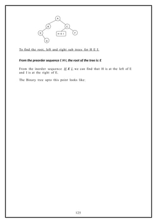
128. The Binary tree upto this point looks like:
n6
n2
n1 n4
n5
n3
n9
n8
n7
Binary Tree Creation and Traversal Using Arrays:
This program performs the following operations:
1. Creates a complete Binary Tree
2. Inorder traversal
3. Preorder traversal
4. Postorder traversal
5. Level order traversal
6. Prints leaf nodes
7. Finds height of the tree created
# include <stdio.h>
# include <stdlib.h>
struct tree
{
struct tree* lchild;
char data[10];
struct tree* rchild;
};
typedef struct tree node;
int ctr;
node *tree[100];
node* getnode()
{
node *temp ;
temp = (node*) malloc(sizeof(node));
printf("n Enter Data: ");
scanf("%s",temp- >data);
temp- >lchild = NULL;
temp- >rchild = NULL;
return temp;
}
void create_fbinarytree()
{
int j, i=0;
printf("n How many nodes you want: ");
scanf("%d",&ctr);
tree[0] = getnode();
j = ctr;
j--;
do
{
if( j > 0 ) /* left child */
139

129. {
tree[ i * 2 + 1 ] = getnode();
tree[i]- >lchild = tree[i * 2 + 1];
j--;
}
if( j > 0 ) /* right child */
{
tree[i * 2 + 2] = getnode();
j--;
tree[i]- >rchild = tree[i * 2 + 2];
}
i++;
} while( j > 0);
}
void inorder(node *root)
{
if( root != NULL )
{
inorder(root- >lchild);
printf("%3s",root- >data);
inorder(root- >rchild);
}
}
void preorder(node *root)
{
if( root != NULL )
{
printf("%3s",root- >data);
preorder(root- >lchild);
preorder(root- >rchild);
}
}
void postorder(node *root)
{
if( root != NULL )
{
postorder(root- >lchild);
postorder(root- >rchild);
printf("%3s",root- >data);
}
}
void levelorder()
{
int j;
for(j = 0; j < ctr; j++)
{
if(tree[j] != NULL)
printf("%3s",tree[j]- >data);
}
}
void print_leaf(node *root)
{
if(root != NULL)
{
if(root- >lchild == NULL && root- >rchild == NULL)
printf("%3s ",root- >data);
print_leaf(root- >lchild);
print_leaf(root- >rchild);
}
}
int height(node *root)
{
if(root == NULL)
{
140

130. return 0;
}
if(root- >lchild == NULL && root- >rchild == NULL)
return 0;
else
return (1 + max(height(root- >lchild), height(root- >rchild)));
}
void main()
{
int i;
create_fbinarytree();
printf("n Inorder Traversal: ");
inorder(tree[0]);
printf("n Preorder Traversal: ");
preorder(tree[0]);
printf("n Postorder Traversal: ");
postorder(tree[0]);
printf("n Level Order Traversal: ");
levelorder();
printf("n Leaf Nodes: ");
print_leaf(tree[0]);
printf("n Height of Tree: %d ", height(tree[0]));
}
Binary Tree Creation and Traversal Using Pointers:
This program performs the following operations:
1. Creates a complete Binary Tree
2. Inorder traversal
3. Preorder traversal
4. Postorder traversal
5. Level order traversal
6. Prints leaf nodes
7. Finds height of the tree created
8. Deletes last node
9. Finds height of the tree created
# include <stdio.h>
# include <stdlib.h>
struct tree
{
struct tree* lchild;
char data[10];
struct tree* rchild;
};
typedef struct tree node;
node *Q[50];
int node_ctr;
node* getnode(void)
{
node *temp ;
temp = (node*) malloc(sizeof(node));
printf("n Enter Data: ");
fflush(stdin);
scanf("%s",temp- >data);
temp- >lchild = NULL;
temp- >rchild = NULL;
return temp;
}
void create_binarytree(node *root)
{
char option;
141

131. if( root != NULL )
{
printf("n Node %s has Left SubTree(Y/N)",root- >data);
fflush(stdin);
scanf("%c",&option);
if( option= = 'Y' || option == 'y')
{
root- >lchild = getnode();
create_binarytree(root- >lchild);
}
else
{
root- >lchild = NULL;
create_binarytree(root- >lchild);
}
printf("n Node %s has Right SubTree(Y/N) ",root- >data);
fflush(stdin);
scanf("%c",&option);
if( option= = 'Y' || option == 'y')
{
root- >rchild = getnode();
create_binarytree(root- >rchild);
}
else
{
root- >rchild = NULL;
create_binarytree(root- >rchild);
}
}
}
void make_Queue(node *root,int parent)
{
if(root != NULL)
{
node_ctr+ +;
Q[parent] = root;
make_Queue(root- >lchild,parent*2 +1);
make_Queue(root- >rchild,parent*2 +2);
}
}
delete_node(node *root, int parent)
{
int index = 0;
if(root == NULL)
printf("n Empty TREE ");
else
{
node_ctr = 0;
make_Queue(root,0);
index = node_ctr- 1;
Q[index] = NULL;
parent = (index- 1) /2;
if( 2* parent + 1 == index )
Q[parent]- >lchild = NULL;
else
Q[parent]- >rchild = NULL;
}
printf("n Node Deleted ..");
}
void inorder(node *root)
{
if(root != NULL)
{
inorder(root- >lchild);
printf("%3s",root- >data);
142

132. inorder(root- >rchild);
}
}
void preorder(node *root)
{
if( root != NULL )
{
printf("%3s",root- >data);
preorder(root- >lchild);
preorder(root- >rchild);
}
}
void postorder(node *root)
{
if( root != NULL )
{
postorder(root- >lchild);
postorder(root- >rchild);
printf("%3s", root- >data);
}
}
void print_leaf(node *root)
{
if(root != NULL)
{
if(root- >lchild == NULL && root- >rchild == NULL)
printf("%3s ",root- >data);
print_leaf(root- >lchild);
print_leaf(root- >rchild);
}
}
int height(node *root)
{
if(root == NULL)
return -1;
else
return (1 + max(height(root- >lchild), height(root- >rchild)));
}
void print_tree(node *root, int line)
{
int i;
if(root != NULL)
{
print_tree(root- >rchild,line+1);
printf("n");
for(i=0;i<line;i+ +)
printf(" ");
printf("%s", root- >data);
print_tree(root- >lchild,line+1);
}
}
void level_order(node *Q[],int ctr)
{
int i;
for( i = 0; i < ctr ; i++)
{
if( Q[i] != NULL )
printf("%5s",Q[i]- >data);
}
}
int menu()
{
int ch;
143

133. clrscr();
printf("n 1. Create Binary Tree ");
printf("n 2. Inorder Traversal ");
printf("n 3. Preorder Traversal ");
printf("n 4. Postorder Traversal ");
printf("n 5. Level Order Traversal");
printf("n 6. Leaf Node ");
printf("n 7. Print Height of Tree ");
printf("n 8. Print Binary Tree ");
printf("n 9. Delete a node ");
printf("n 10. Quit ");
printf("n Enter Your choice: ");
scanf("%d", &ch);
return ch;
}
void main()
{
int i,ch;
node *root = NULL;
do
{
ch = menu();
switch( ch)
{
case 1 :
if( root == NULL )
{
root = getnode();
create_binarytree(root);
}
else
{
printf("n Tree is already Created ..");
}
break;
case 2 :
printf("n Inorder Traversal: ");
inorder(root);
break;
case 3 :
printf("n Preorder Traversal: ");
preorder(root);
break;
case 4 :
printf("n Postorder Traversal: ");
postorder(root);
break;
case 5:
printf("n Level Order Traversal ..");
make_Queue(root,0);
level_order(Q,node_ctr);
break;
case 6 :
printf("n Leaf Nodes: ");
print_leaf(root);
break;
case 7 :
printf("n Height of Tree: %d ", height(root));
break;
case 8 :
printf("n Print Tree n");
print_tree(root, 0);
break;
case 9 :
delete_node(root,0);
break;
case 10 :
exit(0);
144

134. }
getch();
}while(1);
}
Non Recursive Binary Tree Traversal Algorithms:
We can also traverse a binary tree non recursively using stack data
structure for inorder, preorder and postorder.
Inorder Traversal:
Initially push zero onto stack and then set root as vertex. Then repeat the following steps until the
stack is empty:
1. Proceed down the left most path rooted at vertex, pushing each vertex onto the stack and
stop when there is no left son of vertex.
2. Pop and process the nodes on stack if zero is popped then exit. If a
vertex with right son exists, then set right son of vertex as current
vertex and return to step one.
Algorith m inorder()
{
stack[1] = 0
vertex = root
top: while(vertex 0)
≠
{
push the vertex into the stack
vertex = leftson(vertex)
}
pop the element from the stack and make it as vertex
while(vertex 0)
≠
{
print the vertex node
if(rightson(vertex) 0)
≠
{
vertex = rightson(vertex)
goto top
}
pop the element from the stack and made it as vertex
}
}
Preorder Traversal:
Initially push zero onto stack and then set root as vertex. Then repeat the following steps until the
stack is empty:
145

135. 1. Proceed down the left most path by pushing the right son of vertex onto stack, if any and
process each vertex. The traversing ends after a vertex with no left child exists.
2. Pop the vertex from stack, if vertex 0 then return to step one otherwise exit.
≠
Algorith m preorder( )
{
stack[1] = 0
vertex = root.
while(vertex 0)
≠
{
print vertex node
if(rightson(vertex) 0)
≠
push the right son of vertex into the stack.
if(leftson(vertex) 0)
≠
vertex = leftson(vertex)
else
pop the element from the stack and made it as vertex
}
}
Postorder Traversal:
Initially push zero onto stack and then set root as vertex. Then repeat the following steps until the
stack is empty:
1. Proceed down the left most path rooted at vertex. At each vertex of path push vertex on to
stack and if vertex has a right son push –(right son of vertex) onto stack.
2. Pop and process the positive nodes (left nodes). If zero is popped then exit. If a negative
node is popped, then ignore the sign and return to step one.
Algorith m postorder( )
{
stack[1] = 0
vertex = root
top: while(vertex 0)
≠
{
push vertex onto stack
if(rightson(vertex) 0)
≠
push – (vertex) onto stack
vertex = leftson(vertex)
}
pop from stack and make it as vertex
while(vertex > 0)
{
146

136. print the vertex node
pop from stack and make it as vertex
}
if(vertex < 0)
{
vertex = - (vertex)
goto top
}
}
Example 1:
Traverse the following binary tree in pre, post and inorder using non-recursive
traversing algorithm.
A
B
K L
E
G
C
Pr eo r d e r t r a v e rs a l y ie lds:
A, B, D, G , K, H, L, M , C, E
Po st o r d e r t r a v a rs a l y ie lds:
K, G , L, M , H, D, B, E, C, A
I n o r d e r t r a v a rs a l y ie lds:
K, G , D, L, H, M , B, A, E, C
Bi n a ry T r e e Pr e, Po st a n d I n or d er T r av er s i n g
D
H
M
Inorder Traversal:
Initially push zero onto stack and then set root as vertex. Then repeat the following steps until the
stack is empty:
1. Proceed down the left most path rooted at vertex, pushing each vertex onto the stack and
stop when there is no left son of vertex.
2. Pop and process the nodes on stack if zero is popped then exit. If a vertex with right son
exists, then set right son of vertex as current vertex and return to step one.
Current
vertex
Stack Processed nodes Remarks
A 0 PUSH 0
0 A B D G K PUSH the left most path of A
K 0 A B D G K POP K
G 0 A B D K G POP G since K has no right son
D 0 A B K G D POP D since G has no right son
H 0 A B K G D Make the right son of D as vertex
H 0 A B H L K G D PUSH the leftmost path of H
L 0 A B H K G D L POP L
H 0 A B K G D L H POP H since L has no right son
M 0 A B K G D L H Make the right son of H as vertex
0 A B M K G D L H PUSH the left most path of M
147

137. M 0 A B K G D L H M POP M
B 0 A K G D L H M B POP B since M has no right son
A 0 K G D L H M B A Make the right son of A as vertex
C 0 C E K G D L H M B A PUSH the left most path of C
E 0 C K G D L H M B A E POP E
C 0 K G D L H M B A E C Stop since stack is empty
Postorder Traversal:
Initially push zero onto stack and then set root as vertex. Then repeat the following steps until the
stack is empty:
1. Proceed down the left most path rooted at vertex. At each vertex of path push vertex on to
stack and if vertex has a right son push –(right son of vertex) onto stack.
2. Pop and process the positive nodes (left nodes). If zero is popped then exit. If a negative
node is popped, then ignore the sign and return to step one.
Current
vertex
Stack Processed nodes Remarks
A 0 PUSH 0
0 A –C B D –H G K
PUSH the left most path of A with a
-ve for right sons
0 A –C B D –H K G POP all +ve nodes K and G
H 0 A –C B D K G Pop H
0 A –C B D H –M L K G
PUSH the left most path of H with a
-ve for right sons
0 A –C B D H –M K G L POP all +ve nodes L
M 0 A –C B D H K G L Pop M
0 A –C B D H M K G L
PUSH the left most path of M with a
-ve for right sons
0 A –C K G L M H D B POP all +ve nodes M, H, D and B
C 0 A K G L M H D B Pop C
0 A C E K G L M H D B
PUSH the left most path of C with a
-ve for right sons
0 K G L M H D B E C A POP all +ve nodes E, C and A
0 Stop since stack is empty
Preorder Traversal:
Initially push zero onto stack and then set root as vertex. Then repeat the following steps until the
stack is empty:
1. Proceed down the left most path by pushing the right son of vertex onto stack, if any and
process each vertex. The traversing ends after a vertex with no left child exists.
2. Pop the vertex from stack, if vertex 0 then return to step one otherwise exit.
≠
Current
vertex
Stack Processed nodes Remarks
A 0 PUSH 0
0 C H A B D G K
PUSH the right son of each vertex onto stack
and process each vertex in the left most path
148

138. H 0 C A B D G K POP H
0 C M A B D G K H L
PUSH the right son of each vertex onto stack
and process each vertex in the left most path
M 0 C A B D G K H L POP M
0 C A B D G K H L M
PUSH the right son of each vertex onto stack
and process each vertex in the left most path;
M has no left path
C 0 A B D G K H L M Pop C
0 A B D G K H L M C E
PUSH the right son of each vertex onto stack
and process each vertex in the left most path;
C has no right son on the left most path
0 A B D G K H L M C E Stop since stack is empty
Example 2:
Traverse the following binary tree in pre, post and inorder using non-recursive
traversing algorithm.
2
7
6
2 9
5
5
Pr eo r d e r t r a v e rs a l y ie lds:
2 , 7 , 2 , 6 , 5 , 1 1 , 5 , 9 , 4
Po st o r d e r t r a v a rs a l y ie lds:
2 , 5 , 1 1 , 6 , 7 , 4 , 9 , 5 , 2
I n o r d e r t r a v a rs a l y ie lds:
2 , 7 , 5 , 6 , 1 1 , 2 , 5 , 4 , 9
Bi n a ry T r e e Pr e, Po st a n d I n or d er T r av er s i n g
4
1 1
Inorder Traversal:
Initially push zero onto stack and then set root as vertex. Then repeat the following steps until the
stack is empty:
1. Proceed down the left most path rooted at vertex, pushing each vertex onto the stack and
stop when there is no left son of vertex.
2. Pop and process the nodes on stack if zero is popped then exit. If a vertex with right son
exists, then set right son of vertex as current vertex and return to step one.
Current
vertex
Stack Processed nodes Remarks
2 0
0 2 7 2
2 0 2 7 2
7 0 2 2 7
6 0 2 6 5 2 7
5 0 2 6 2 7 5
11 0 2 2 7 5 6 11
149

139. 5 0 5 2 7 5 6 11 2
9 0 9 4 2 7 5 6 11 2 5
4 0 9 2 7 5 6 11 2 5 4
0 2 7 5 6 11 2 5 4 9 Stop since stack is empty
Postorder Traversal:
Initially push zero onto stack and then set root as vertex. Then repeat the following steps until the
stack is empty:
1. Proceed down the left most path rooted at vertex. At each vertex of path push vertex on to
stack and if vertex has a right son push –(right son of vertex) onto stack.
2. Pop and process the positive nodes (left nodes). If zero is popped then exit. If a negative
node is popped, then ignore the sign and return to step one.
Current
vertex
Stack Processed nodes Remarks
2 0
0 2 –5 7 –6 2
2 0 2 –5 7 –6 2
6 0 2 –5 7 2
0 2 –5 7 6 –11 5 2
5 0 2 –5 7 6 –11 2 5
11 0 2 –5 7 6 11 2 5
0 2 –5 2 5 11 6 7
5 0 2 5 –9 2 5 11 6 7
9 0 2 5 9 4 2 5 11 6 7
0 2 5 11 6 7 4 9 5 2 Stop since stack is empty
Preorder Traversal:
Initially push zero onto stack and then set root as vertex. Then repeat the following steps until the
stack is empty:
1. Proceed down the left most path by pushing the right son of vertex onto stack, if any and
process each vertex. The traversing ends after a vertex with no left child exists.
2. Pop the vertex from stack, if vertex 0 then return to step one otherwise exit.
≠
Current
vertex
Stack Processed nodes Remarks
2 0
0 5 6 2 7 2
6 0 5 11 2 7 2 6 5
11 0 5 2 7 2 6 5
0 5 2 7 2 6 5 11
5 0 9 2 7 2 6 5 11
9 0 2 7 2 6 5 11 5
0 2 7 2 6 5 11 5 9 4 Stop since stack is empty
150

140. 7.4. Expression Trees:
Expression tree is a binary tree, because all of the operations are binary. It is also possible for a node
to have only one child, as is the case with the unary minus operator. The leaves of an expression tree
are operands, such as constants or variable names, and the other (non leaf) nodes contain operators.
Once an expression tree is constructed we can traverse it in three ways:
 Inorder Traversal
 Preorder Traversal
 Postorder Traversal
Figure 7.4.1 shows some more expression trees that represent arithmetic expressions given in infix
form.
/
b
+
c
a
+
d
+
+
c
+
d
b
a
-
+ *
/
+
+
x
a
*
y a
c
b
( a) ( a + b) + ( c / d)
(c ) ( (- a) + ( x + y ) ) / ( ( + b ) * ( c * a) )
( b) ( ( a + b) + c ) + d
Fi g ur e 7. 4. 1 Ex pr e s s i o n T r e e s
An expression tree can be generated for the infix and postfix expressions.
An algorithm to convert a postfix expression into an expression tree is as follows:
1. Read the expression one symbol at a time.
2. If the symbol is an operand, we create a one-node tree and push a pointer to it onto a
stack.
3. If the symbol is an operator, we pop pointers to two trees T1 and T2 from the stack (T1 is
popped first) and form a new tree whose root is the operator and whose left and right
children point to T2 and T1 respectively. A pointer to this new tree is then pushed onto
the stack.
Example 1:
Construct an expression tree for the postfix expression: a b + c d e + * *
The first two symbols are operands, so we create one-node trees and push pointers to them onto a
stack.
151

141. a b
Next, a ‘+’ is read, so two pointers to trees are popped, a new tree is formed, and a pointer to it is
pushed onto the stack.
a b
+
b
Next, c, d, and e are read, and for each one–node tree is created and a pointer to the corresponding
tree is pushed onto the stack.
a b
+
b c d e
Now a ‘+’ is read, so two trees are merged.
a b
+
b
c
d e
+ +
Continuing, a ‘*’ is read, so we pop two tree pointers and form a new tree with a ‘*’ as root.
a
+
b c
d e
+
+
e
*
Finally, the last symbol is read, two trees are merged, and a pointer to the final tree is left on the
stack.
152

142. a
+
b c
d
e
+
+
e
*
*
For the above tree:
Inorder form of the expression: a + b * c * d + e
Preorder form of the expression: * + a b * c + d e
Postorder form of the expression: a b + c d e + * *
Example 2:
Construct an expression tree for the arithmetic expression:
(A + B * C) – ((D * E + F) / G)
Solution:
First convert the infix expression into postfix notation.
Postfix notation of the arithmetic expression is: A B C * + D E * F + G / -
The first three symbols are operands, so we create one-node trees and pointers to three nodes
pushed onto the stack.
A B C
Next, a ‘*’ is read, so two pointers to trees are popped, a new tree is formed, and a pointer to it is
pushed onto the stack.
B
A *
C
Next, a ‘+’ is read, so two pointers to trees are popped, a new tree is formed, and a pointer to it is
pushed onto the stack.
153

143. B
A
*
C
+
Next, D and E are read, and for each one–node tree is created and a pointer to the corresponding
tree is pushed onto the stack.
B
A
*
C
+ E
D
Continuing, a ‘*’ is read, so we pop two tree pointers and form a new tree with a ‘*’ as root.
A
B C
D
+
* E
*
Proceeding similar to the previous steps, finally, when the last symbol is read, the expression tree is
as follows:
154

144. A
+
B
* G
C
+ /
*
-
+
F
D E
UNIT- 5 GRAPHS
Graph G is a pair (V, E), where V is a finite set of vertices and E is a finite set of edges. We will often
denote n = |V|, e = |E|.
A graph is generally displayed as figure 7.5.1, in which the vertices are
represented by circles and the edges by lines.
An edge with an orientation (i.e., arrow head) is a directed edge, while
an edge with no orientation is our undirected edge.
If all the edges in a graph are undirected, then the graph is an
undirected graph. The graph of figures 7.5.1(a) is undirected graphs. If
all the edges are directed; then the graph is a directed graph. The graph
of figure 7.5.1(b) is a directed graph. A directed graph is also called as
digraph.
A graph G is connected if and only if there is a simple path between any
two nodes in G.
A graph G is said to be complete if every node a in G is adjacent to every
other node v in G. A complete graph with n nodes will have n(n- 1)/2
edges. For example, Figure 7.5.1.(a) and figure 7.5.1.(d) are complete
graphs.
155

145. A directed graph G is said to be connected, or strongly connected, if for
each pair u, v for nodes in G there is a path from u to v and there is a
path from v to u. On the other hand, G is said to be unilaterally
connected if for any pair u, v of nodes in G there is a path from u to v or
a path from v to u. For example, the digraph shown in figure 7.5.1 (e) is
strongly connected.
A B
C D
E
B D
G
E
C
F
A
Fi g ur e 7. 5. 1 V ar i o u s Gr a p h s
( b)
( a)
v 4 v 2
v 3
v 1
( d)
v 4 v 2
v 3
v 1
(c )
( f )
v 4 v 2
v 3
v 1 v 1
v 2 v 3
v 4 v 5 v 6 v 7
( g)
( e)
v 4 v 2
v 3
v 1
We can assign weight function to the edges: wG (e) is a weight of edge e  E. The graph which has
such function assigned is called weighted graph.
The number of incoming edges to a vertex v is called in–degree of the vertex (denote indeg(v)). The
number of outgoing edges from a vertex is called out-degree (denote outdeg(v)). For example, let us
consider the digraph shown in figure 7.5.1(f),
indegree(v1) = 2outdegree(v1) = 1
indegree(v2) = 2outdegree(v2) = 0
A path is a sequence of vertices (v1, v2, . . . . . . , vk), where for all i, (vi, vi+1)  E. A path is simple if all
vertices in the path are distinct. If there a path containing one or more edges which starts from a
vertex Vi and terminates into the same vertex then the path is known as a cycle. For example, there is
a cycle in figure 7.5.1 (a), figure 7.5.1 (c) and figure 7.5.1 (d).
If a graph (digraph) does not have any cycle then it is called acyclic graph. For example, the graphs
of figure 7.5.1 (f) and figure 7.5.1 (g) are acyclic graphs.
A graph G’ = (V’
, E’
) is a sub-graph of graph G = (V, E) iff V’  V and E’  E.
A Forest is a set of disjoint trees. If we remove the root node of a given tree then it becomes forest.
The following figure shows a forest F that consists of three trees T1, T2 and T3.
156

146. A graph that has either self loop or parallel edges or both is called multi-graph.
Tree is a connected acyclic graph (there aren’t any sequences of edges that go around in a loop). A
spanning tree of a graph G = (V, E) is a tree that contains all vertices of V and is a subgraph of G. A
single graph can have multiple spanning trees.
Let T be a spanning tree of a graph G. Then
1. Any two vertices in T are connected by a unique simple path.
2. If any edge is removed from T, then T becomes disconnected.
3. If we add any edge into T, then the new graph will contain a cycle.
4. Number of edges in T is n-1.
Representation of Graphs:
There are two ways of representing digraphs. They are:
 Adjacency matrix.
 Adjacency List.
 Incidence matrix.
Adjacency matrix:
In this representation, the adjacency matrix of a graph G is a two dimensional n x n matrix, say A =
(ai,j), where




otherwise
v
to
v
from
edge
an
is
there
if
a
j
i
j
i
0
1
,
The matrix is symmetric in case of undirected graph, while it may be asymmetric if the graph is
directed. This matrix is also called as Boolean matrix or bit matrix.
1
4
3
2
5
Fig ur e 7. 5. 2. A gr a p h a n d it s A d j ac e nc y m a t r ix
G1 :
( a)
Figure 7.5.2(b) shows the adjacency matrix representation of the graph G1 shown in figure 7.5.2(a).
The adjacency matrix is also useful to store multigraph as well as weighted graph. In case of
A
D
B
E
C F
Q
P
R
X
Y
Z
T2 T3
T1
A Fore st F
1 2 3 4 5
1 0 1 1 0 1
2 0 0 1 1 1
3 0 0 0 1 0
4 0 0 0 0 0
5 0 0 1 1 0
(b)
157

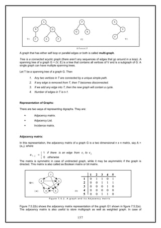
147. multigraph representation, instead of entry 0 or 1, the entry will be between number of edges between
two vertices.
In case of weighted graph, the entries are weights of the edges between the vertices. The adjacency
matrix for a weighted graph is called as cost adjacency matrix. Figure 7.5.3(b) shows the cost
adjacency matrix representation of the graph G2 shown in figure 7.5.3(a).
B D
G
E
C
F
A
6
3
2
4
1
2 1
4
1
2
4
2
Fi g ur e 7. 5. 3 W e i g h t e d gr a p h a n d it s Co st a d j ac e nc y m a t r i x
( a)
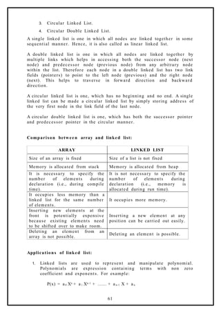
Adjacency List :
In this representation, the n rows of the adjacency matrix are
represented as n linked lists. An array Adj[1, 2, . . . . . n] of pointers
where for 1 < v < n, Adj[v] points to a linked list containing the vertices
which are adjacent to v (i.e. the vertices that can be reached from v by a
single edge). If the edges have weights then these weights may also be
stored in the linked list elements. For the graph G in figure 7.5.2 (a), the
adjacency list in shown in figure 7.5.4 (b).
1
0
1 1
0 1
0 0
1
3
2
1
1
3
2
1
2
3
3
3
1 2
2
( a) A d j ac e nc y M at r i x ( b) A d j ac e nc y Li st
Fi g ur e 7. 5. 4 A d j ac e n c y m a t r i x a n d a d j ac e nc y l i st
Incidence Matrix:
In this representation, if G is a graph with n vertices, e edges and no self loops, then incidence matrix
A is defined as an n by e matrix, say A = (ai,j), where




otherwise
v
to
incident
j
edge
an
is
there
if
a i
j
i
0
1
,
Here, n rows correspond to n vertices and e columns correspond to e edges. Such a matrix is called
as vertex-edge incidence matrix or simply incidence matrix.
A B C D E F G
A 0 3 6    
B 3 0 2 4   
C 6 2 0 1 4 2 
D  4 1 0 2  4
E   4 2 0 2 1
F   2  2 0 1
G    4 1 1 0
G2:
(b)
158

148. B D
G
E
C
F
A
g
a
b
c
d
k l
f
i
e
h
j
Fi g ur e 7. 5. 4 Gr a p h a n d it s i nc i d e nc e m a t r i x
( a)
( b)
Figure 7.5.4(b) shows the incidence matrix representation of the graph G1 shown in figure 7.5.4(a).
7.6. Minimum Spanning Tree (MST):
A spanning tree for a connected graph is a tree whose vertex set is the same as the vertex set of the
given graph, and whose edge set is a subset of the edge set of the given graph. i.e., any connected
graph will have a spanning tree.
Weight of a spanning tree w(T) is the sum of weights of all edges in T. Minimum spanning tree (MST)
is a spanning tree with the smallest possible weight.
Example:
G:
A gr a p h G:
T hr e e ( of m a n y p o s s i b l e) s p a n n i n g t r e e s f r o m gr a p h G:
5
2
4
6
1
3
A w e i g ht e d gr a p h G: T h e m i n i m a l s p a n n i n g t r e e f r o m w e i g ht e d gr a p h G:
2
3
1
G:
Let's consider a couple of real-world examples on minimum spanning tree:
 One practical application of a MST would be in the design of a network. For instance, a
group of individuals, who are separated by varying distances, wish to be connected
together in a telephone network. Although MST cannot do anything about the distance
from one connection to another, it can be used to determine the least cost paths with no
cycles in this network, thereby connecting everyone at a minimum cost.
 Another useful application of MST would be finding airline routes. The vertices of the
graph would represent cities, and the edges would represent routes between the cities.
MST can be applied to optimize airline routes by finding the least costly paths with no
cycles.
Minimum spanning tree, can be constructed using any of the following two algorithms:
a b c d e f g h i j k l
A 1 0 0 0 0 0 1 0 0 0 0 0
B 1 1 1 0 0 0 0 0 0 0 0 0
C 0 1 0 1 0 0 1 1 0 0 1 0
D 0 0 1 1 1 1 0 0 0 0 0 0
E 0 0 0 0 1 0 0 1 1 1 0 0
F 0 0 0 0 0 0 0 0 0 1 1 1
G 0 0 0 0 0 1 0 0 1 0 0 1
159

149. 1. Kruskal’s algorithm and
2. Prim algorithm.
Both algorithms differ in their methodology, but both eventually end up with the MST. Kruskal's
algorithm uses edges, and Prim’s algorithm uses vertex connections in determining the MST.
7.6.1. Kruskal’s Algorithm
This is a greedy algorithm. A greedy algorithm chooses some local optimum (i.e. picking an edge with
the least weight in a MST).
Kruskal's algorithm works as follows: Take a graph with 'n' vertices, keep on adding the shortest
(least cost) edge, while avoiding the creation of cycles, until (n - 1) edges have been added.
Sometimes two or more edges may have the same cost.
The order in which the edges are chosen, in this case, does not matter. Different MST’s may result,
but they will all have the same total cost, which will always be the minimum cost.
Kruskal’s Algorithm for minimal spanning tree is as follows:
1. Make the tree T empty.
2. Repeat the steps 3, 4 and 5 as long as T contains less than n - 1
edges and E is not empty otherwise, proceed to step 6.
3. Choose an edge (v, w) from E of lowest cost.
4. Delete (v, w) from E.
5. If (v, w) does not create a cycle in T
then Add (v, w) to T
else discard (v, w)
6. If T contains fewer than n - 1 edges then print no spanning tree.
Example 1:
Construct the minimal spanning tree for the graph shown below:
3
5
2
1
6
4
15
50
10
30
20
35
45 40
25
55
Arrange all the edges in the increasing order of their costs:
Cost 10 15 20 25 30 35 40 45 50 55
Edge (1, 2) (3, 6) (4, 6) (2, 6) (1, 4) (3, 5) (2, 5) (1, 5) (2, 3) (5, 6)
The stages in Kruskal’s algorithm for minimal spanning tree is as follows:
160

150. Edge Cost Stages in Kruskal’s algorithm Remarks
(1, 2) 10
2
1
3
4
5
6
The edge between vertices 1 and 2 is the
first edge selected. It is included in the
spanning tree.
(3, 6) 15
2
1
6
5
3
4
Next, the edge between vertices 3 and 6
is selected and included in the tree.
(4, 6) 20
2
1
6
5
3
4
The edge between vertices 4 and 6 is
next included in the tree.
(2, 6) 25
2
1
6
5
3
4
The edge between vertices 2 and 6 is
considered next and included in the tree.
(1, 4) 30
Reject
The edge between the vertices 1 and 4 is
discarded as its inclusion creates a cycle.
(3, 5) 35
2
1
6
5
3
4
Finally, the edge between vertices 3 and
5 is considered and included in the tree
built. This completes the tree.
The cost of the minimal spanning tree is
105 .
Example 2:
Construct the minimal spanning tree for the graph shown below:
1
2
3
6
5
4
7
2 8
1 0
1 6
1 2
2 2
2 5
2 4
1 4
1 8
Solution:
161

151. Arrange all the edges in the increasing order of their costs:
Cost 10 12 14 16 18 22 24 25 28
Edge (1, 6) (3, 4) (2, 7) (2, 3) (4, 7) (4, 5) (5, 7) (5, 6) (1, 2)
The stages in Kruskal’s algorithm for minimal spanning tree is as follows:
Edge Cost Stages in Kruskal’s algorithm Remarks
(1, 6) 10
2
1
3
4
5
6
7
The edge between vertices 1 and 6 is the
first edge selected. It is included in the
spanning tree.
(3, 4) 12
2
1
3
4
5
6
7
Next, the edge between vertices 3 and 4
is selected and included in the tree.
(2, 7) 14
2
1
3
4
5
6
7
The edge between vertices 2 and 7 is
next included in the tree.
(2, 3) 16
2
1
3
4
5
6
7
The edge between vertices 2 and 3 is
next included in the tree.
(4, 7) 18 Reject
The edge between the vertices 4 and 7 is
discarded as its inclusion creates a cycle.
(4, 5) 22
2
1
3
4
5
6
7
The edge between vertices 4 and 7 is
considered next and included in the tree.
(5, 7) 24
Reject
The edge between the vertices 5 and 7 is
discarded as its inclusion creates a cycle.
162

152. (5, 6) 25
2
1
3
4
5
6
7
Finally, the edge between vertices 5 and 6 is
considered and included in the tree built. This
completes the tree.
The cost of the minimal spanning tree is
99 .
7.6.2. Reachability Matrix (Warshall’s Algorithm) :
Warshall’s algorithm requires to know which edges exist and which do
not. It doesn’t need to know the lengths of the edges in the given
directed graph. This information is conveniently displayed by adjacency
matrix for the graph, in which a ‘1’ indicates the existence of an edge
and ‘0’ indicates non- existence.
A d j ac e nc y M at r i x W a r s h a l l’ s A l g or it h m
A l l Pa ir s Rec h a b i l it y
M at r i x
It begins with the adjacency matrix for the given graph, which is called
A0, and then updates the matrix ‘n’ times, producing matrices called A1,
A2, . . . . . , An and then stops.
In warshall’s algorithm the matrix Ai merely contains information about
the existence of i – paths. A 1 entry in the matrix Ai will correspond to the
existence of an i – paths and O entry will correspond to non- existence.
Thus when the algorithm stops, the final matrix, the matrix An, contains
the desired connectivity information.
A 1 entry indicates a pair of vertices, which are connected, and O entry
indicates a pair, which are not. This matrix is called a reachability matrix
or path matrix for the graph. It is also called the transitive closure of the
original adjacency matrix.
The update rule for computing Ai from Ai-1 in warshall’s algorithm is:
Ai [x, y] = Ai-1 [x, y] ۷ (Ai-1 [x, i] ٨ Ai-1 [i, y]) ---- (1)
Example 1:
Use warshall’s algorithm to calculate the reachability matrix for the
graph:
163

153. 3
2
1 4
1 1
4
7
7
5
1
6
We begin with the adjacency matrix of the graph ‘A0’















0
1
1
1
0
0
0
0
1
1
0
0
0
1
1
0
4
3
2
1
0
A
The first step is to compute ‘A1’ matrix. To do so we will use the updating
rule – (1).
Before doing so we notice that only 1 entry in A0 must remain 1 in A1,
since in Boolean algebra 1 + (any thing) = 1. Since these are only nine 0
entries in A0, there are only nine entries in A0 that need to be updated.
A1[1, 1] = A0[1, 1] ۷ (A0[1, 1] ٨ A0[1, 1]) = 0 ۷ (0 ٨ 0) = 0
A1[2, 1] = A0[2, 1] ۷ (A0[2, 1] ٨ A0[1, 1]) = 0 ۷ (0 ٨ 0) = 0
A1[2, 2] = A0[2, 2] ۷ (A0[2, 1] ٨ A0[1, 2]) = 0 ۷ (0 ٨ 1) = 0
A1[3, 1] = A0[3, 1] ۷ (A0[3, 1] ٨ A0[1, 1]) = 0 ۷ (0 ٨ 0) = 0
A1[3, 2] = A0[3, 2] ۷ (A0[3, 1] ٨ A0[1, 2]) = 0 ۷ (0 ٨ 1) = 0
A1[3, 3] = A0[3, 3] ۷ (A0[3, 1] ٨ A0[1, 3]) = 0 ۷ (0 ٨ 1) = 0
A1[3, 4] = A0[3, 4] ۷ (A0[3, 1] ٨ A0[1, 4]) = 0 ۷ (0 ٨ 0) = 0
A1[4, 4] = A0[4, 4] ۷ (A0[4, 1] ٨ A0[1, 4]) = 0 ۷ (1 ٨ 0) = 0















0
1
1
1
0
0
0
0
1
1
0
0
0
1
1
0
4
3
2
1
1
A
Next, A2 must be calculated from A1; but again we need to update the 0
entries,
A2[1, 1] = A1[1, 1] ۷ (A1[1, 2] ٨ A1[2, 1]) = 0 ۷ (1 ٨ 0) = 0
A2[1, 4] = A1[1, 4] ۷ (A1[1, 2] ٨ A1[2, 4]) = 0 ۷ (1 ٨ 1) = 1
A2[2, 1] = A1[2, 1] ۷ (A1[2, 2] ٨ A1[2, 1]) = 0 ۷ (0 ٨ 0) = 0
A2[2, 2] = A1[2, 2] ۷ (A1[2, 2] ٨ A1[2, 2]) = 0 ۷ (0 ٨ 0) = 0
A2[3, 1] = A1[3, 1] ۷ (A1[3, 2] ٨ A1[2, 1]) = 0 ۷ (0 ٨ 0) = 0
A2[3, 2] = A1[3, 2] ۷ (A1[3, 2] ٨ A1[2, 2]) = 0 ۷ (0 ٨ 0) = 0
164

154. A2[3, 3] = A1[3, 3] ۷ (A1[3, 2] ٨ A1[2, 3]) = 0 ۷ (0 ٨ 1) = 0
A2[3, 4] = A1[3, 4] ۷ (A1[3, 2] ٨ A1[2, 4]) = 0 ۷ (0 ٨ 1) = 0
A2[4, 4] = A1[4, 4] ۷ (A1[4, 2] ٨ A1[2, 4]) = 0 ۷ (1 ٨ 1) = 1















1
1
1
1
0
0
0
0
1
1
0
0
1
1
1
0
4
3
2
1
2
A
This matrix has only seven 0 entries, and so to compute A3, we need to do
only seven computations.
A3[1, 1] = A2[1, 1] ۷ (A2[1, 3] ٨ A2[3, 1]) = 0 ۷ (1 ٨ 0) = 0
A3[2, 1] = A2[2, 1] ۷ (A2[2, 3] ٨ A2[3, 1]) = 0 ۷ (1 ٨ 0) = 0
A3[2, 2] = A2[2, 2] ۷ (A2[2, 3] ٨ A2[3, 2]) = 0 ۷ (1 ٨ 0) = 0
A3[3, 1] = A2[3, 1] ۷ (A2[3, 3] ٨ A2[3, 1]) = 0 ۷ (0 ٨ 0) = 0
A3[3, 2] = A2[3, 2] ۷ (A2[3, 3] ٨ A2[3, 2]) = 0 ۷ (0 ٨ 0) = 0
A3[3, 3] = A2[3, 3] ۷ (A2[3, 3] ٨ A2[3, 3]) = 0 ۷ (0 ٨ 0) = 0
A3[3, 4] = A2[3, 4] ۷ (A2[3, 3] ٨ A2[3, 4]) = 0 ۷ (0 ٨ 0) = 0















1
1
1
1
0
0
0
0
1
1
0
0
1
1
1
0
4
3
2
1
3
A
Once A3 is calculated, we use the update rule to calculate A4 and stop.
This matrix is the reachability matrix for the graph.
A4[1, 1] = A3 [1, 1] ۷ (A3 [1, 4] ٨ A3 [4, 1]) = 0 ۷ (1 ٨ 1) = 0 ۷ 1 = 1
A4[2, 1] = A3 [2, 1] ۷ (A3 [2, 4] ٨ A3 [4, 1]) = 0 ۷ (1 ٨ 1) = 0 ۷ 1 = 1
A4[2, 2] = A3 [2, 2] ۷ (A3 [2, 4] ٨ A3 [4, 2]) = 0 ۷ (1 ٨ 1) = 0 ۷ 1 = 1
A4[3, 1] = A3 [3, 1] ۷ (A3 [3, 4] ٨ A3 [4, 1]) = 0 ۷ (0 ٨ 1) = 0 ۷ 0 = 0
A4[3, 2] = A3 [3, 2] ۷ (A3 [3, 4] ٨ A3 [4, 2]) = 0 ۷ (0 ٨ 1) = 0 ۷ 0 = 0
A4[3, 3] = A3 [3, 3] ۷ (A3 [3, 4] ٨ A3 [4, 3]) = 0 ۷ (0 ٨ 1) = 0 ۷ 0 = 0
A4[3, 4] = A3 [3, 4] ۷ (A3 [3, 4] ٨ A3 [4, 4]) = 0 ۷ (0 ٨ 1) = 0 ۷ 0 = 0















1
1
1
1
0
0
0
0
1
1
1
1
1
1
1
1
4
3
2
1
4
A
165

155. Note that according to the algorithm vertex 3 is not reachable from itself
1. This is because as can be seen in the graph, there is no path from
vertex 3 back to itself.
7.6.3. Traversin g a Graph:
Many graph algorithms require one to systematically examine the nodes and edges of a graph G.
There are two standard ways to do this. They are:
 Breadth first traversal (BFT)
 Depth first traversal (DFT)
The BFT will use a queue as an auxiliary structure to hold nodes for future processing and the DFT
will use a STACK.
During the execution of these algorithms, each node N of G will be in one
of three states, called the status of N, as follows:
1. STATUS = 1 (Ready state): The initial state of the node N.
2. STATUS = 2 (Waiting state): The node N is on the QUEUE or
STACK, waiting to be processed.
3. STATUS = 3 (Processed state): The node N has been processed.
Both BFS and DFS impose a tree (the BFS/DFS tree) on the structure of
graph. So, we can compute a spanning tree in a graph. The computed
spanning tree is not a minimum spanning tree. The spanning trees
obtained using depth first searches are called depth first spanning trees.
The spanning trees obtained using breadth first searches are called
Breadth first spanning trees.
Breadth first search and traversal:
The general idea behind a breadth first traversal beginning at a starting
node A is as follows. First we examine the starting node A. Then we
examine all the neighbors of A. Then we examine all the neighbors of
neighbors of A. And so on. We need to keep track of the neighbors of a
node, and we need to guarantee that no node is processed more than
once. This is accomplished by using a QUEUE to hold nodes that are
waiting to be processed, and by using a field STATUS that tells us the
current status of any node. The spanning trees obtained using BFS are
called Breadth first spanning trees.
Breadth first traversal algorithm on graph G is as follows:
This algorithm executes a BFT on graph G beginning at a starting node A.
1. Initialize all nodes to the ready state (STATUS = 1).
2. Put the starting node A in QUEUE and change its status to the
waiting state (STATUS = 2).
166

156. 3. Repeat the following steps until QUEUE is empty:
a. Remove the front node N of QUEUE. Process N and change
the status of N to the processed state (STATUS = 3).
b. Add to the rear of QUEUE all the neighbors of N that are in
the ready state (STATUS = 1), and change their status to the
waiting state (STATUS = 2).
4. Exit.
Depth first search and traversal:
Depth first search of undirected graph proceeds as follows: First we
examine the starting node V. Next an unvisited vertex 'W' adjacent to 'V'
is selected and a depth first search from 'W' is initiated. When a vertex
'U' is reached such that all its adjacent vertices have been visited, we
back up to the last vertex visited, which has an unvisited vertex 'W'
adjacent to it and initiate a depth first search from W. The search
terminates when no unvisited vertex can be reached from any of the
visited ones.
This algorithm is similar to the inorder traversal of binary tree. DFT
algorithm is similar to BFT except now use a STACK instead of the
QUEUE. Again field STATUS is used to tell us the current status of a
node.
The algorithm for depth first traversal on a graph G is as follows.
This algorithm executes a DFT on graph G beginning at a starting node A.
1. Initialize all nodes to the ready state (STATUS = 1).
2. Push the starting node A into STACK and change its status to the
waiting state (STATUS = 2).
3. Repeat the following steps until STACK is empty:
a. Pop the top node N from STACK. Process N and change the
status of N to the processed state (STATUS = 3).
b. Push all the neighbors of N that are in the ready state
(STATUS = 1), and change their status to the waiting state
(STATUS = 2).
4. Exit.
Example 1:
Consider the graph shown below. Traverse the graph shown below in breadth first order and depth
first order.
167

157. A
C B
F
G
E
D
K
J
A Gr a p h G
Breadth- first search and traversal:
The steps involved in breadth first traversal are as follows:
Curre
nt
Node
QUEUE
Processed
Nodes
Status
A B C D E F G J K
1 1 1 1 1 1 1 1 1
A 2 1 1 1 1 1 1 1 1
A F C B A 3 2 2 1 1 2 1 1 1
F C B D A F 3 2 2 2 1 3 1 1 1
C
B D E
G
A F C 3 2 3 2 2 3 2 1 1
B D E G A F C B 3 3 3 2 2 3 2 1 1
D E G J A F C B D 3 3 3 3 2 3 2 2 1
E G J K A F C B D E 3 3 3 3 3 3 2 2 2
G J K A F C B D E G 3 3 3 3 3 3 3 2 2
J K A F C B D E G J 3 3 3 3 3 3 3 3 2
K EMPTY
A F C B D E G J
K
3 3 3 3 3 3 3 3 3
For the above graph the Breadth first traversal sequence is: A F C B D E G J K.
Depth-first search and traversal:
The steps involved in depth first traversal are as follows:
Curre
nt
Node
Stack
Processed
Nodes
Status
A B C D E F G J K
1 1 1 1 1 1 1 1 1
A 2 1 1 1 1 1 1 1 1
A B C F A 3 2 2 1 1 2 1 1 1
F B C D A F 3 2 2 2 1 3 1 1 1
Nod
e
Adjacen cy
List
A F, C, B
B A, C, G
C
A, B, D, E, F,
G
D C, F, E, J
E C, D, G, J, K
F A, C, D
G B, C, E, K
J D, E, K
K E, G, J
Adjacency list for graph G
168

158. D B C E J A F D 3 2 2 3 2 3 1 2 1
J B C E
K
A F D J
3 2 2 3 2 3 1 3 2
K B C E
G
A F D J K
3 2 2 3 2 3 2 3 3
G B C E A F D J K G 3 2 2 3 2 3 3 3 3
E B C A F D J K G E 3 2 2 3 3 3 3 3 3
C B A F D J K G E C 3 2 3 3 3 3 3 3 3
B EMPTY A F D J K G E C
B
3 3 3 3 3 3 3 3 3
For the above graph the Depth first traversal sequence is: A F D J K G E C B.
Example 2:
Traverse the graph shown below in breadth first order, depth first order and construct the breadth first
and depth first spanning trees.
A
D
F
B C G
H I
J K
L M
E
The Gr aph G
If the depth first traversal is initiated from vertex A, then the vertices of
graph G are visited in the order: A F E D G L J K M H I C B . The depth
first spanning tree is shown in the figure given below:
A
B
F
D
E
G
L H C
J I
K M
D e p t h f ir s t T r a v e r s a l
Node Adjacency List
A F, B, C, G
B A
C A, G
D E, F
E G, D, F
F A, E, D
G A, L, E, H, J, C
H G, I
I H
J G, L, K, M
K J
L G, J, M
M L, J
The adjacency list for the graph G
169

159. If the breadth first traversal is initiated from vertex A, then the vertices
of graph G are visited in the order: A F B C G E D L H J M I K . The
breadth first spanning tree is shown in the figure given below:
A
B
F C G
H
E D L
M
J
K
I
Br e a dt h f ir st t r av er s a l
Example 3:
Traverse the graph shown below in breadth first order, depth first order and construct the breadth first
and depth first spanning trees.
7
8
1
3
6
5
2
4
Gr a p h G
Vert e x
1
2
3
4
5
6
7
8
2 3
4
1
6
1
8
2
2
3
3
4
8
8
8
5 6 7
5
7
Adj acency list fo r gr aph G
If the depth first is initiated from vertex 1, then the vertices of graph G
are visited in the order: 1, 2, 4, 8, 5, 6, 3, 7. The depth first spanning tree
is as follows:
170

160. 7
8
1
3
6
5
2
4
De p t h F ir st S p a n n i n g T r e e
Breadth first search and traversal:
If the breadth first search is initiated from vertex 1, then the vertices of
G are visited in the order: 1, 2, 3, 4, 5, 6, 7, 8. The breadth first spanning
tree is as follows:
7.7. General Trees (m- ary tree):
If in a tree, the outdegree of every node is less than or equal to m , the
tree is called an m- ary tree. If the outdegree of every node is exactly
equal to m or zero then the tree is called a full or complete m- ary tree.
For m = 2, the trees are called binary and full binary trees.
Differences between trees and binary trees:
TREE BINARY TREE
Each element in a tree can have any number of
subtrees.
Each element in a binary tree has at most two
subtrees.
The subtrees in a tree are unordered.
The subtrees of each element in a binary tree
are ordered (i.e. we distinguish between left and
right subtrees).
7
8
1
3
6
5
2
4
Br e a dt h F ir st S p a n n i n g T r e e
171

161. Converting a m- ary tree (general tree) to a binary tree:
There is a one- to-one mapping between general ordered trees and binary
trees. So, every tree can be uniquely represented by a binary tree.
Furthermore, a forest can also be represented by a binary tree.
Conversion from general tree to binary can be done in two stages.
 As a first step, we delete all the branches originating in every
node except the left most branch.
 We draw edges from a node to the node on the right, if any,
which is situated at the same level.
 Once this is done then for any particular node, we choose its left
and right sons in the following manner:
 The left son is the node, which is immediately below the
given node, and the right son is the node to the immediate
right of the given node on the same horizontal line. Such a
binary tree will not have a right subtree.
Example 1:
Convert (Encoding m-ary trees as binary trees) the following ordered tree into a binary tree.
6 7 8 9 1 0 1 1
2 3 4 5
1
Solution:
Stage 1 tree using the above mentioned procedure is as follows:
6 7 8 9 1 0 1 1
2 3 4 5
1
Stage 2 tree using the above mentioned procedure is as follows:
172

162. 1
2
6 3
7 8 4
5
9
1 0
1 1
Example 2:
Construct a unique binary tree from the given forest.
4 5 6
8 9
1 0
2 3
1 1
7
1
1 0
1 2 1 3
Solution:
Stage 1 tree using the above mentioned procedure is as follows:
4 5 6
8 9
2 3
1 1
7
1
1 0
1 2 1 3
Stage 2 tree using the above mentioned procedure is as follows (binary tree representation of forest):
173

163. 4
5 6
8
9
2
3
7
1
1 0
1 2
1 3
9
1 1
Search and Traversal Techniqu e s for m- ary trees:
Search involves visiting nodes in a tree in a systematic manner, and may or may not result into a visit
to all nodes. When the search necessarily involved the examination of every vertex in the tree, it is
called the traversal. Traversing of a tree can be done in two ways.
1. Depth first search or traversal.
2. Breadth first search or traversal.
Depth first search:
In Depth first search, we begin with root as a start state, then some
successor of the start state, then some successor of that state, then some
successor of that and so on, trying to reach a goal state. One simple way
to implement depth first search is to use a stack data structure
consisting of root node as a start state.
If depth first search reaches a state S without successors, or if all the
successors of a state S have been chosen (visited) and a goal state has
not get been found, then it “backs up” that means it goes to the
immediately previous state or predecessor formally, the state whose
successor was ‘S’ originally.
To illustrate this let us consider the tree shown below.
S
A
D
E
B
C
H
F
I
J
G
K
G OA L
ST A RT
Suppose S is the start and G is the only goal state. Depth first search will
174

164. first visit S, then A, then D. But D has no successors, so we must back up
to A and try its second successor, E. But this doesn’t have any successors
either, so we back up to A again. But now we have tried all the
successors of A and haven’t found the goal state G so we must back to
‘S’. Now ‘S’ has a second successor, B. But B has no successors, so we
back up to S again and choose its third successor, C. C has one
successor, F. The first successor of F is H, and the first of H is J. J doesn’t
have any successors, so we back up to H and try its second successor.
And that’s G, the only goal state.
So the solution path to the goal is S, C, F, H and G and the states
considered were in order S, A, D, E, B, C, F, H, J, G.
Disadvantages:
1. It works very fine when search graphs are trees or lattices, but
can get struck in an infinite loop on graphs. This is because
depth first search can travel around a cycle in the graph
forever.
To eliminate this keep a list of states previously visited, and
never permit search to return to any of them.
2. We cannot come up with shortest solution to the problem.
Breadth first search:
Breadth-first search starts at root node S and “discovers" which vertices are reachable from S.
Breadth-first search discovers vertices in increasing order of distance. Breadth-first search is named
because it visits vertices across the entire breadth.
To illustrate this let us consider the following tree:
S
A
D
E
B
C
H
F
I
J
G
K
G OA L
ST A RT
Breadth first search finds states level by level. Here we first check all the
immediate successors of the start state. Then all the immediate
successors of these, then all the immediate successors of these, and so
on until we find a goal node. Suppose S is the start state and G is the
goal state. In the figure, start state S is at level 0; A, B and C are at level
1; D, e and F at level 2; H and I at level 3; and J, G and K at level 4.
175

165. So breadth first search, will consider in order S, A, B, C, D, E, F, H, I, J
and G and then stop because it has reached the goal node.
Breadth first search does not have the danger of infinite loops as we
consider states in order of increasing number of branches (level) from
the start state.
One simple way to implement breadth first search is to use a queue data
structure consisting of just a start state.
7.8. Sparse Matrices:
A sparse matrix is a two–dimensional array having the value of majority elements as
null. The density of the matrix is the number of non-zero elements divided by the
total number of matrix elements. The matrices with very low density are often good
for use of the sparse format. For example,















0
4
0
0
0
0
3
1
0
0
2
0
5
0
0
0
A
As far as the storage of a sparse matrix is concerned, storing of null elements is
nothing but wastage of memory. So we should devise technique such that only non-
null elements will be stored.
The matrix A produces:
(3, 1) 1
(2, 2) 2
S = (3, 2) 3
(4, 3) 4
(1, 4) 5
The printed output lists the non-zero elements of S, together with their row and
column indices. The elements are sorted by columns, reflecting the internal data
structure.
In large number of applications, sparse matrices are involved. One approach is to
use the linked list.
The program to represent sparse matrix:
/* Check whether the given matrix is sparse matrix or not, if so then
print in alternative form for storage. */
# include <stdio.h>
# include <conio.h>
176

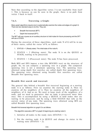
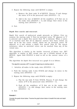
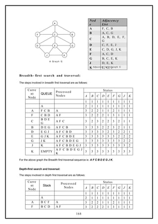
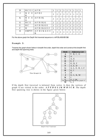
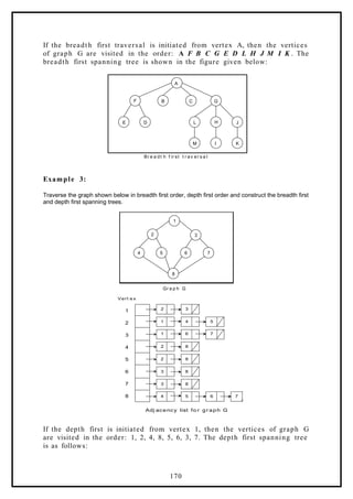
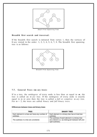
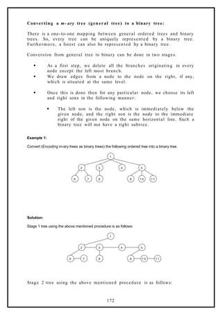
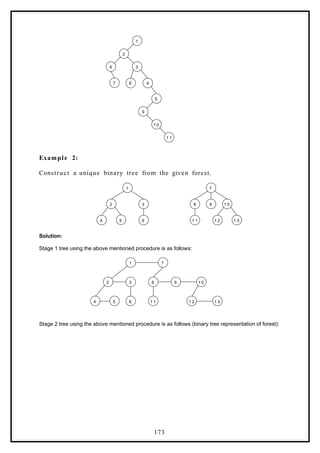
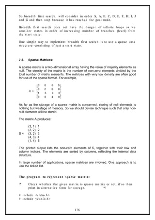
166. main()
{
int matrix[20][20], m, n, total_elements, total_zeros = 0, i, j;
clrscr();
printf("n Enter Number of rows and columns: ");
scanf("%d %d",&m, &n);
total_elements = m * n;
printf("n Enter data for sparse matrix: ");
for(i = 0; i < m ; i++)
{
for( j = 0; j < n ; j++)
{
scanf("%d", &matrix[i][j]);
if( matrix[i][j] == 0)
{
total_zeros + +;
}
}
}
if(total_zeros > total_elements/2 )
{
printf("n Given Matrix is Sparse Matrix..");
printf("n The Representaion of Sparse Matrix is: n");
printf("n Row t Col t Value ");
for(i = 0; i < m ; i++)
{
for( j = 0; j < n ; j++)
{
if( matrix[i][j] != 0)
{
printf("n %d t %d t %d",i,j,matrix[i][j]);
}
}
}
}
else
printf("n Given Matrix is Not a Sparse Matrix..");
}
177