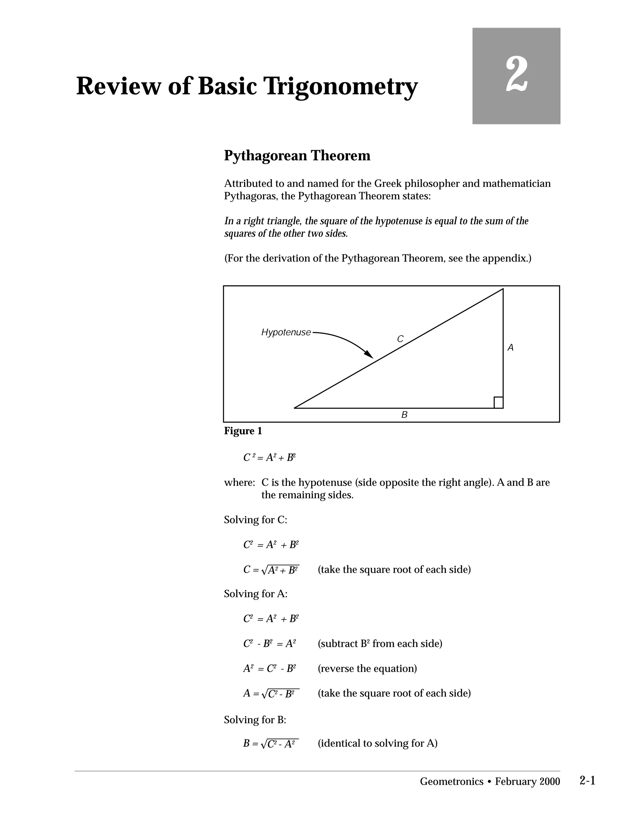
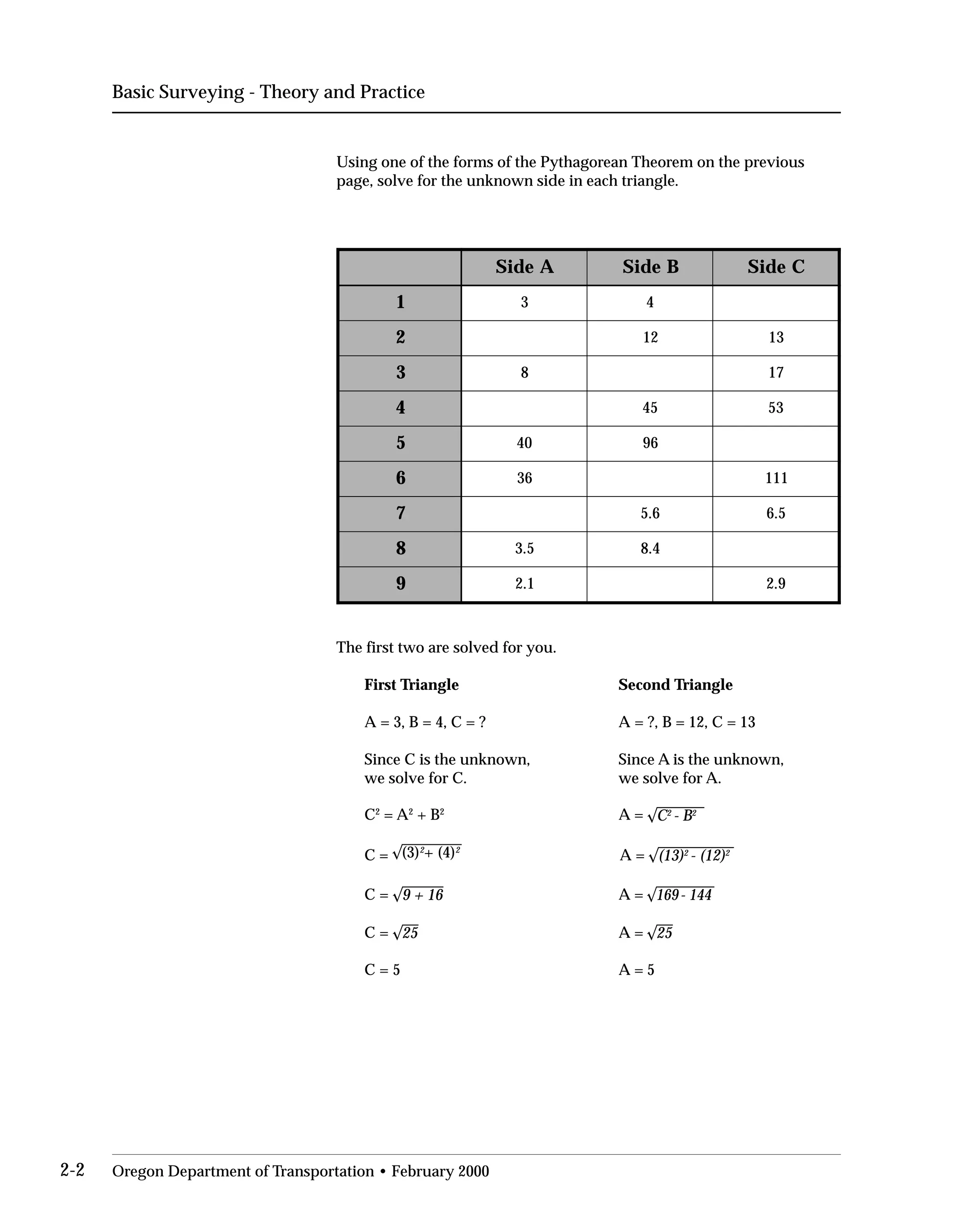
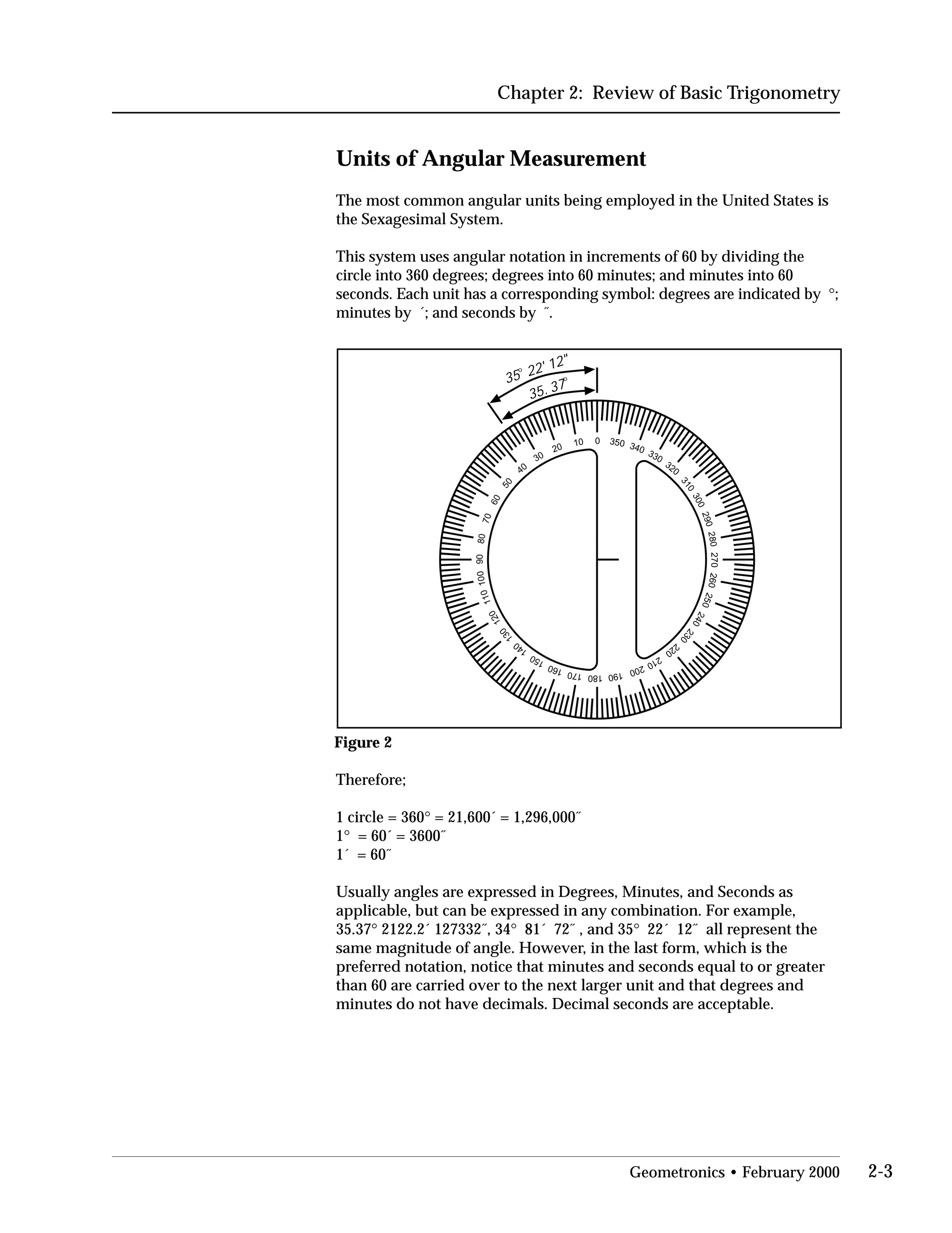
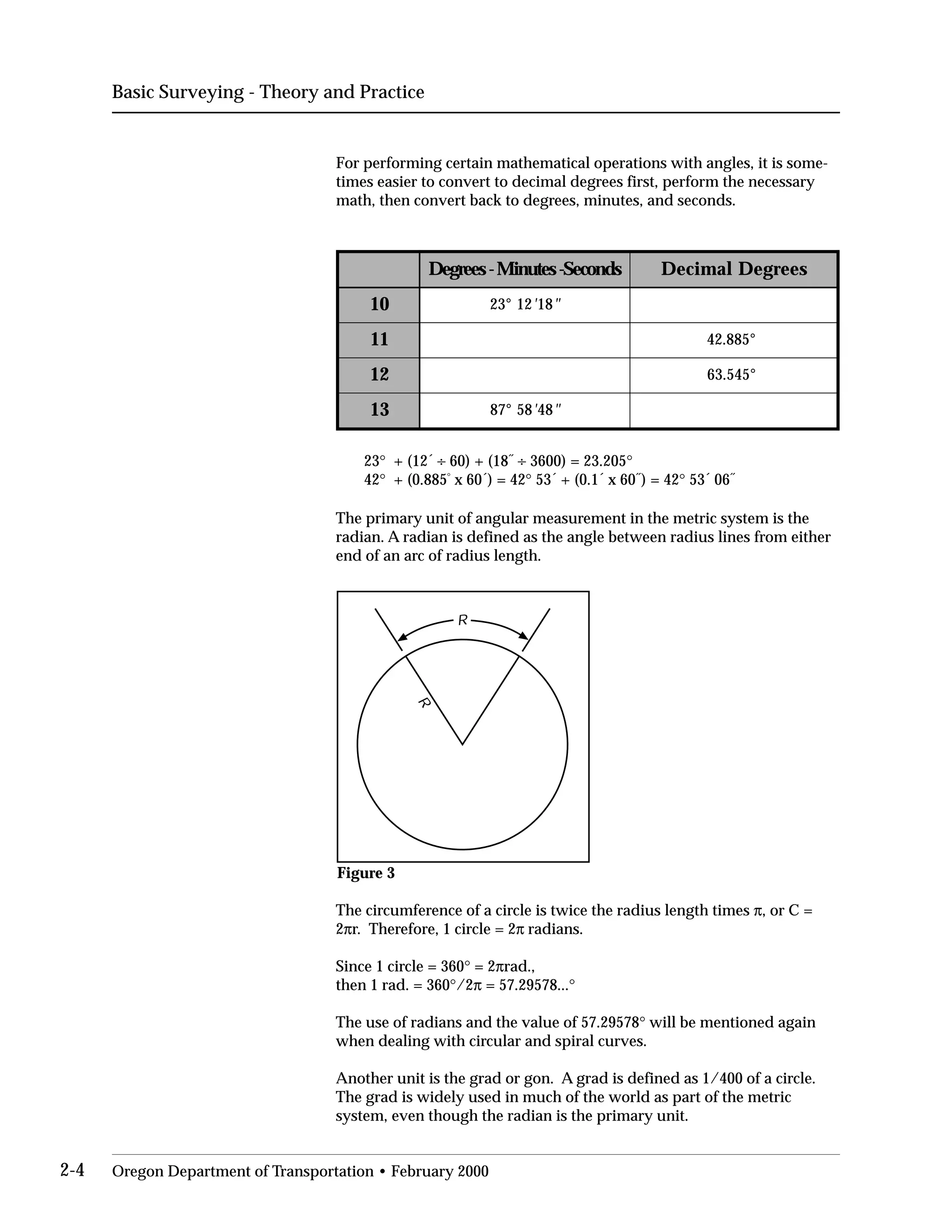
This document provides an overview of basic trigonometry concepts used in surveying. It defines the Pythagorean theorem and shows how to solve for unknown sides of right triangles. It also describes units of angular measurement, including degrees-minutes-seconds and their relationships. Finally, it explains conversions between sexagesimal and decimal degrees and introduces radians as a unit of angular measurement.

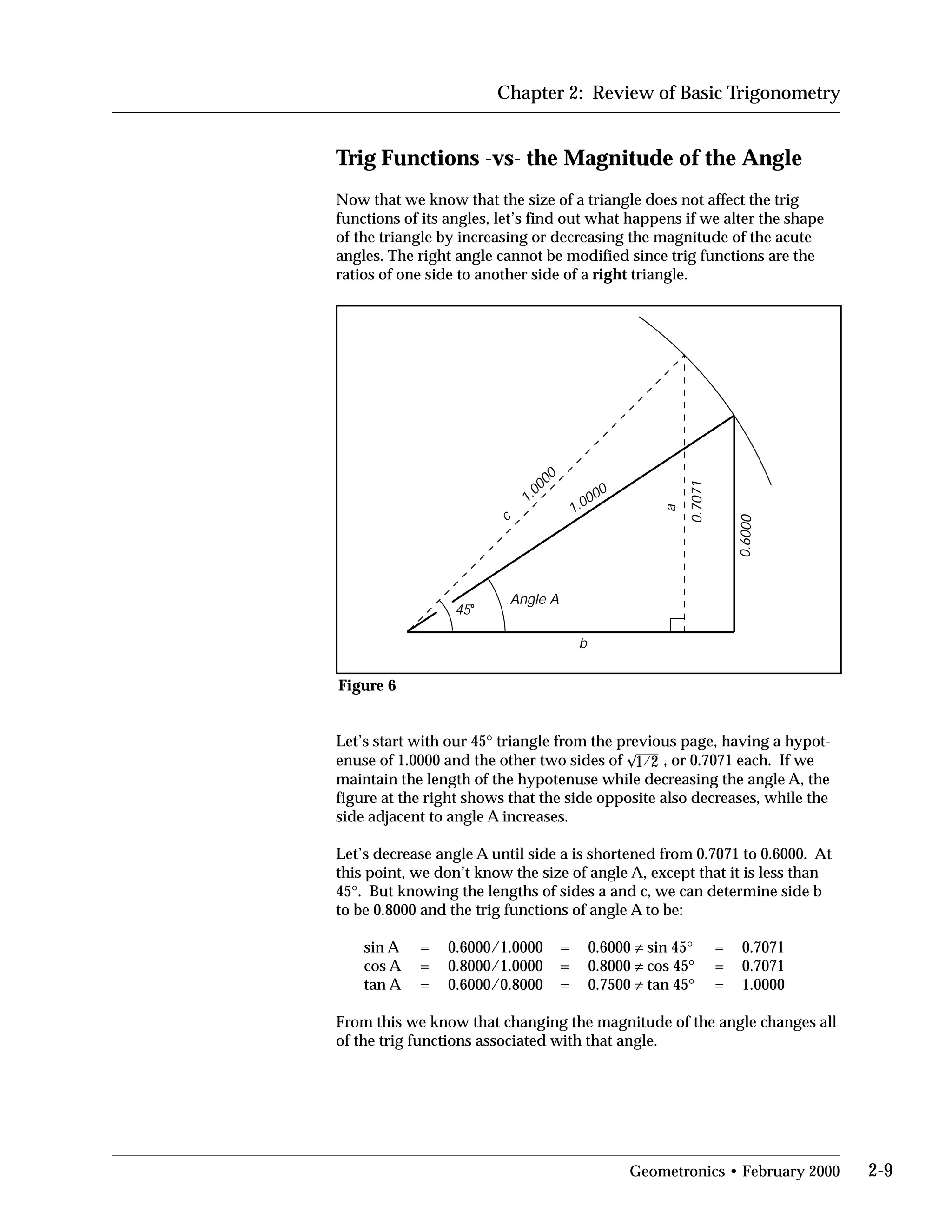
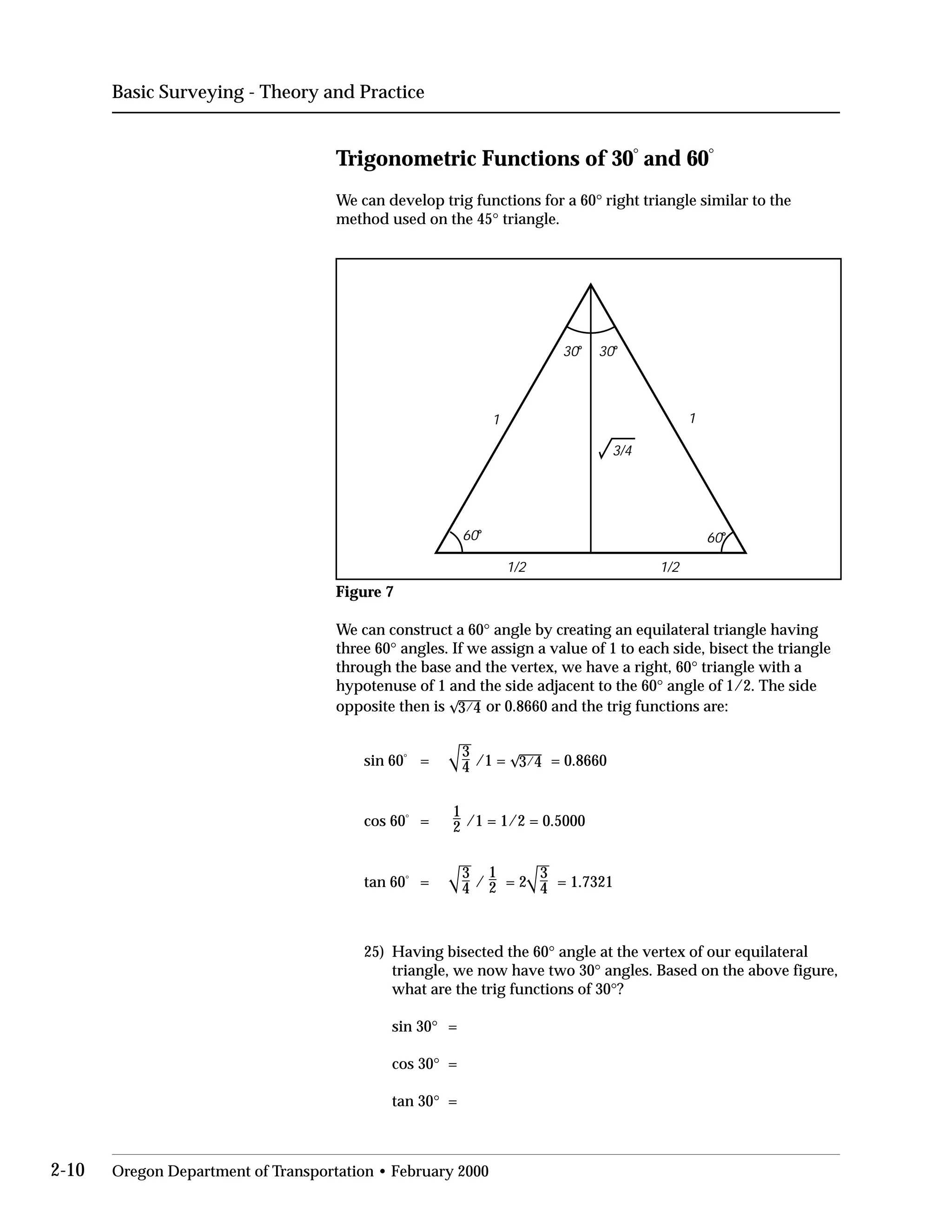
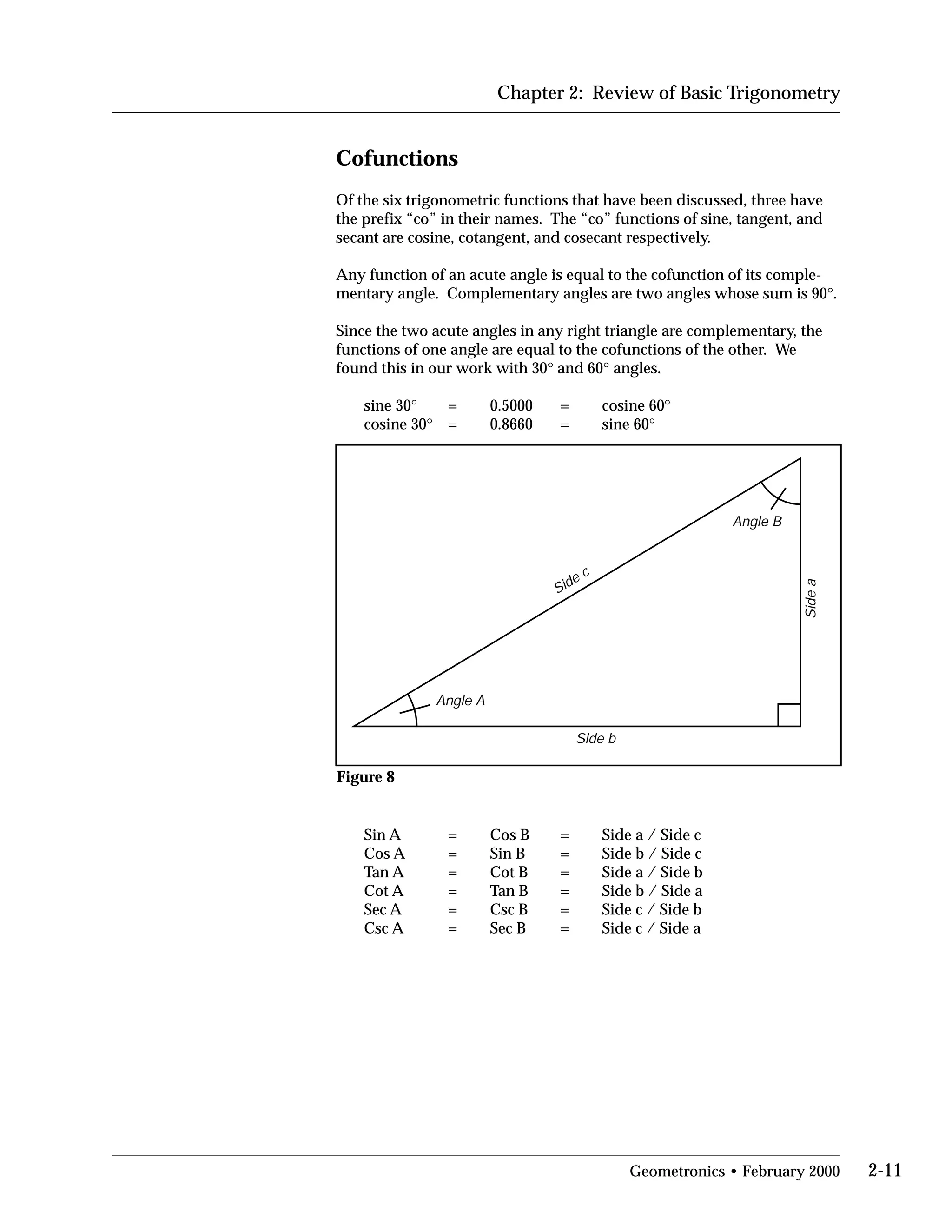
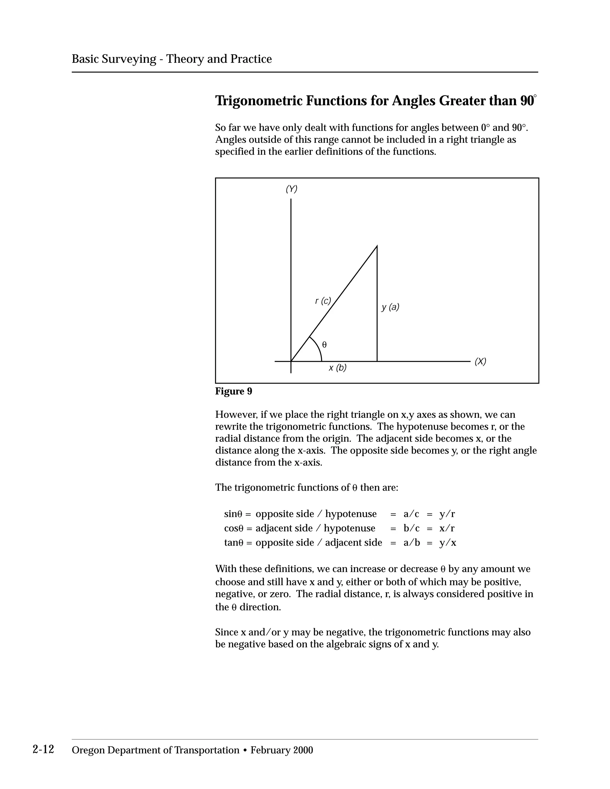


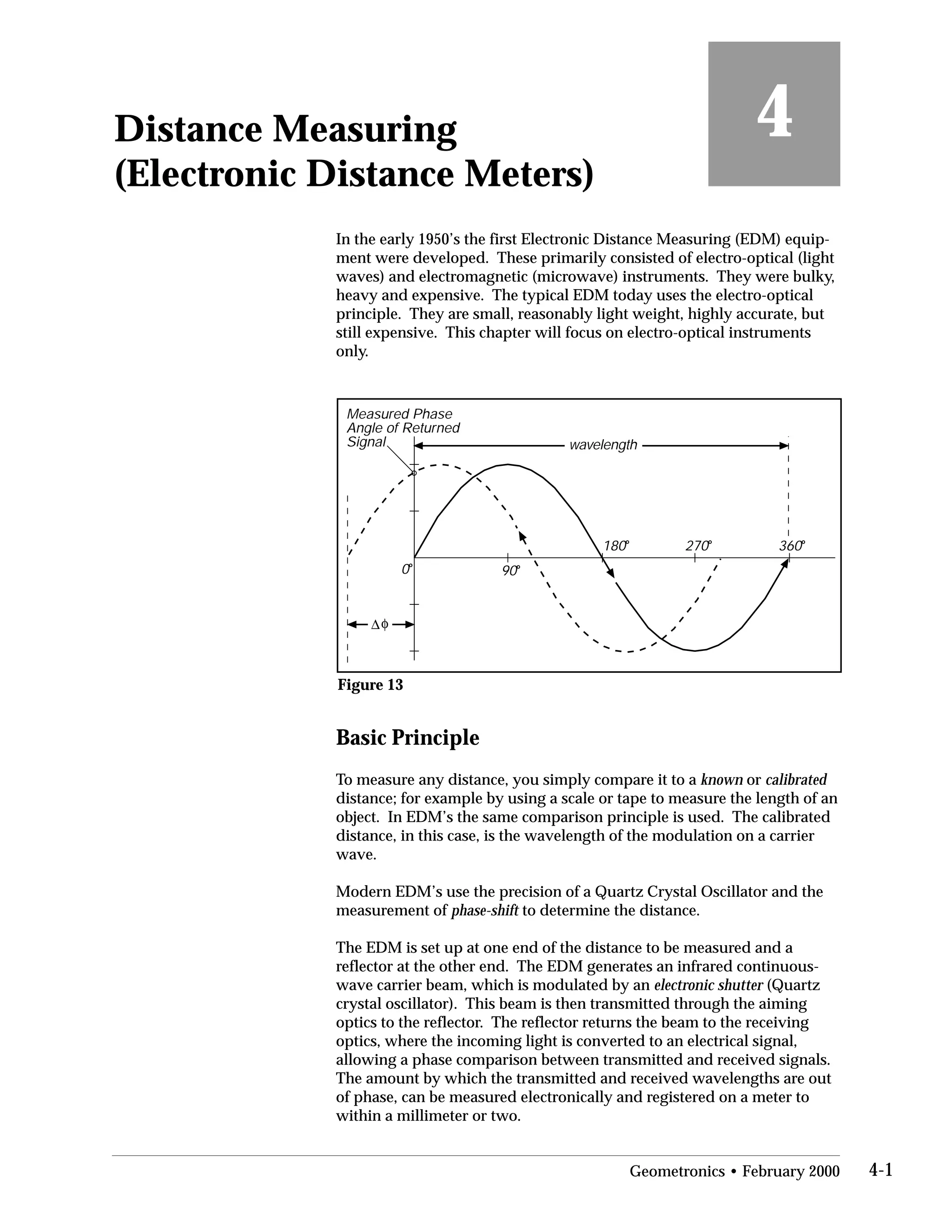


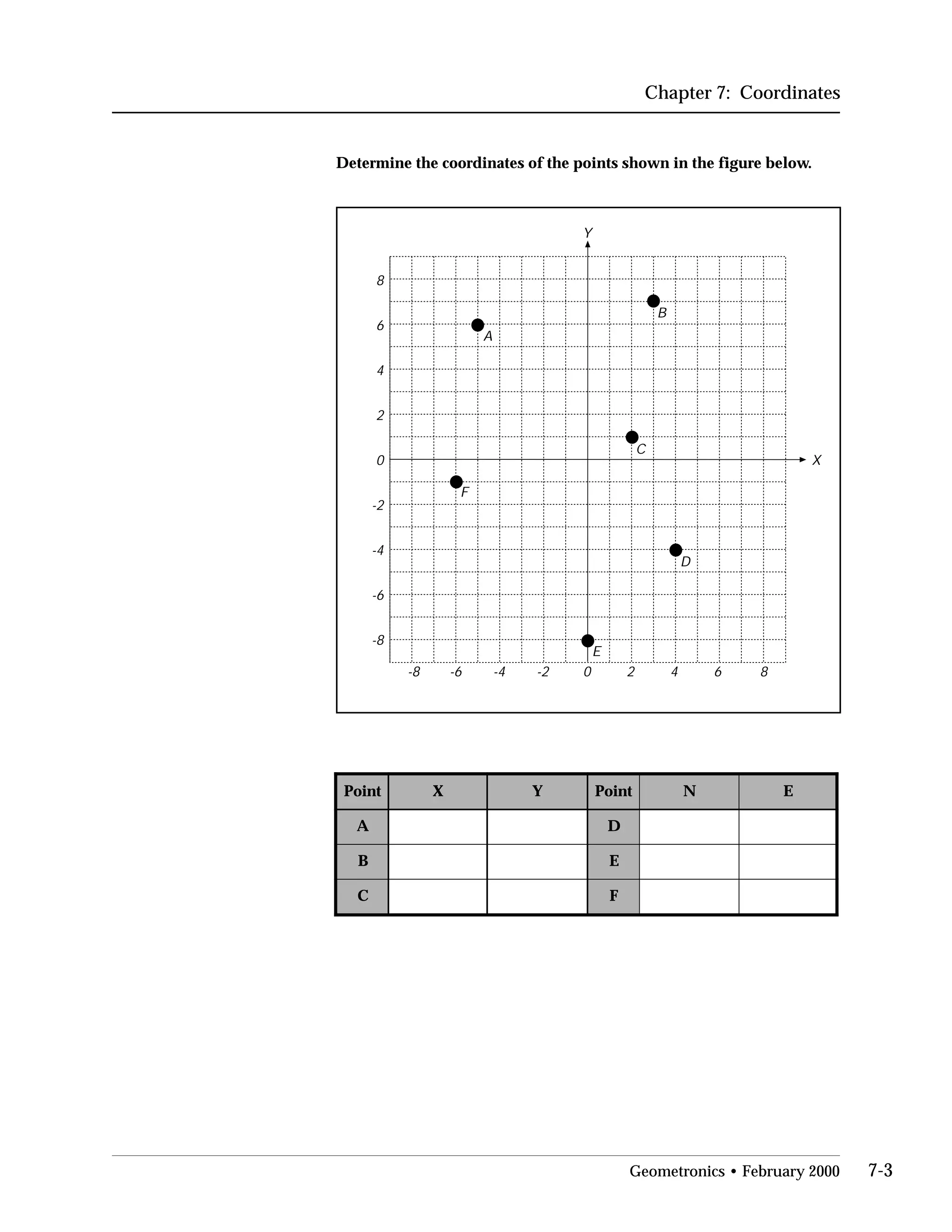
![Chapter 7: Coordinates
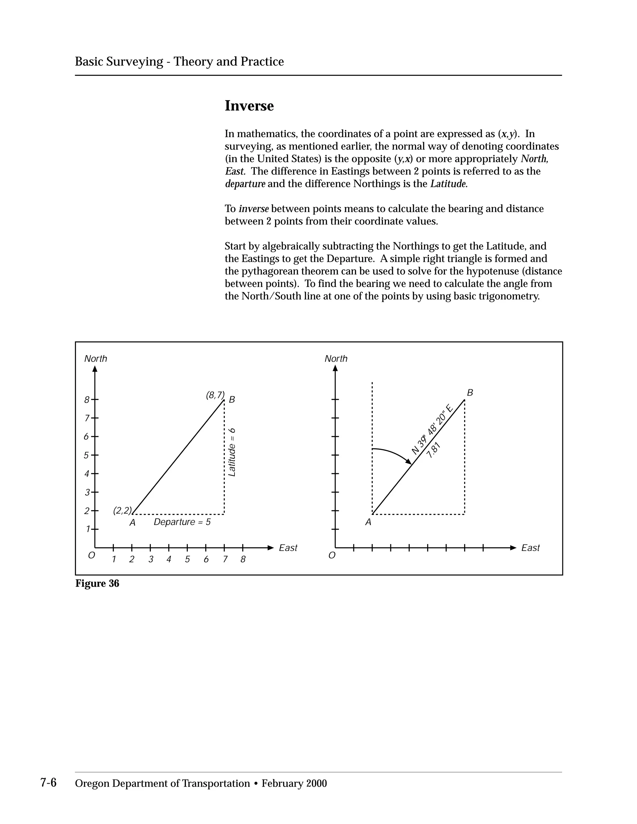
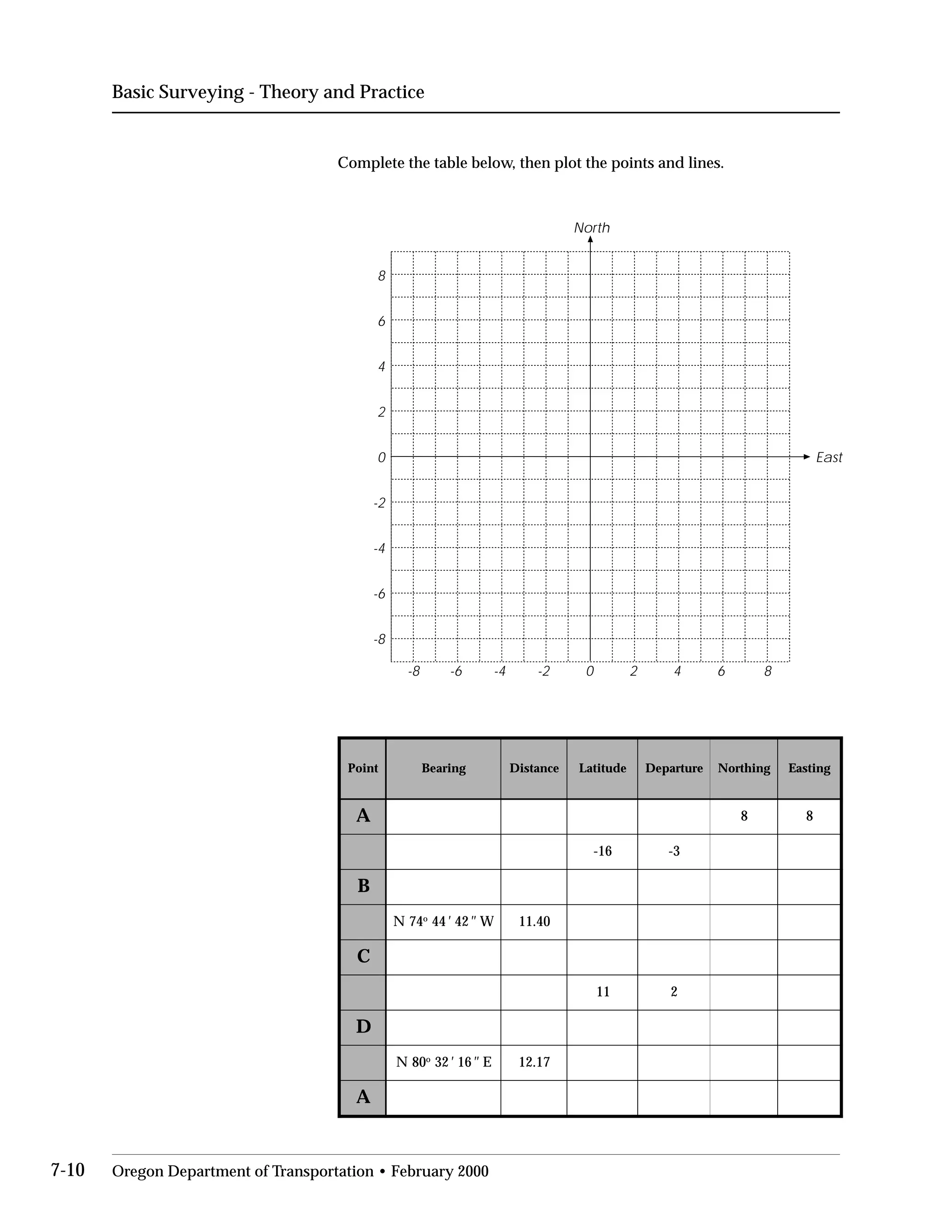
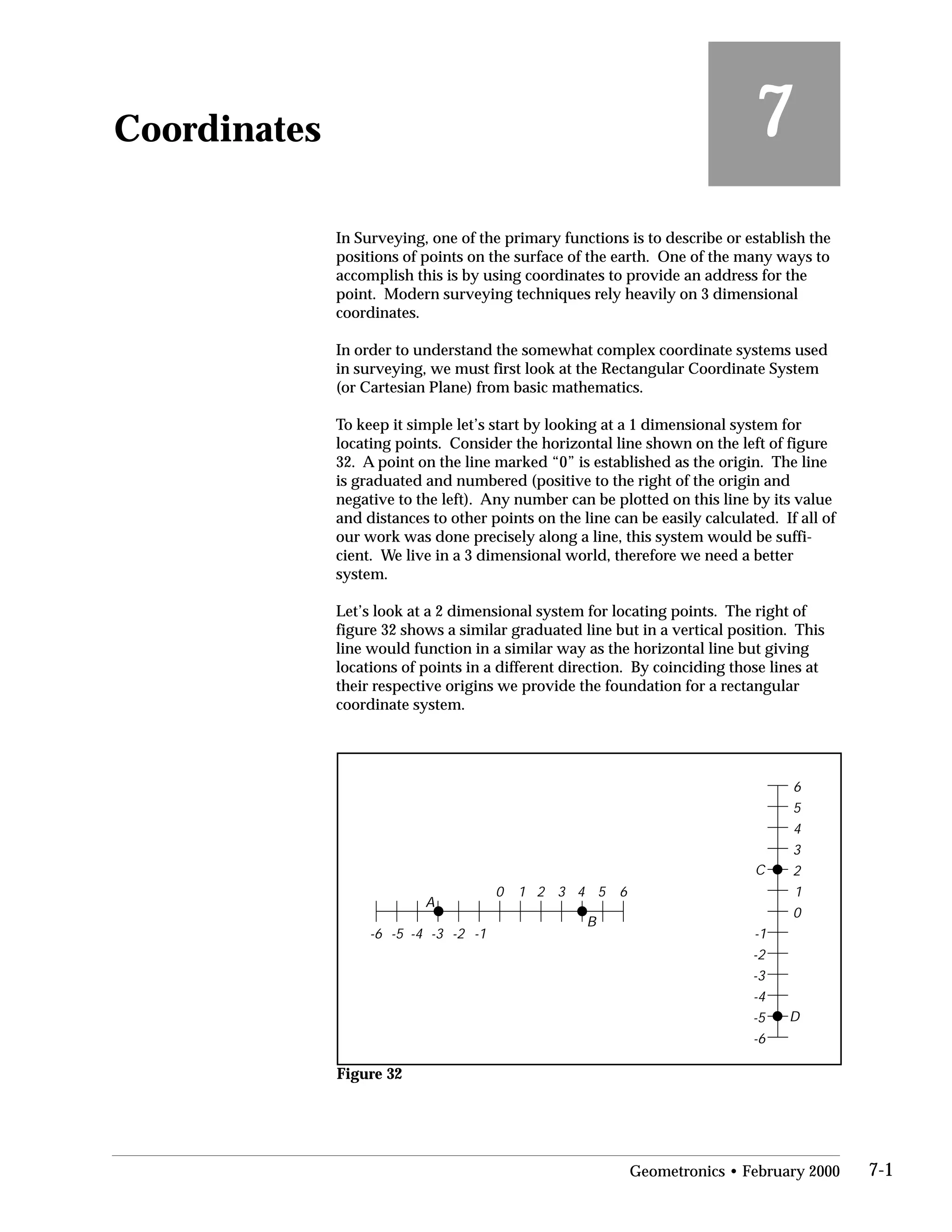
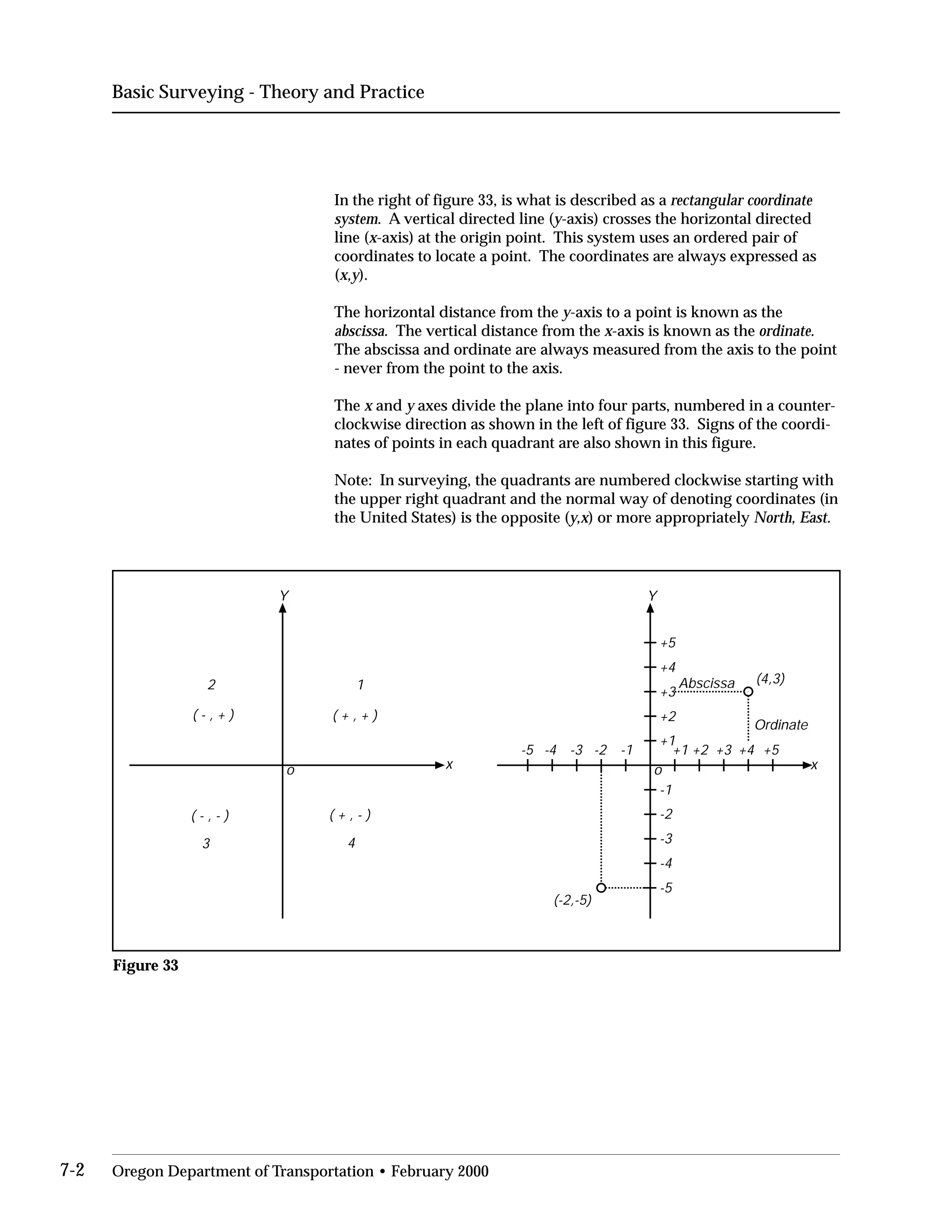
Measuring distance between coordinates
When determining the distance between any two points in a rectangular
coordinate system, the pythagorean theorem may be used (see Review of
Basic Trigonometry). In the figure below, the distance between A and B
can be computed in the following way :
AB = [4-(-2)]2
+[3-(-5)]2
AB = [4+2)]2
+[3+5)]2
AB = 10
CB=+4-(-2)=4+2 AC=+3-(-5)=3+5
Point C in this figure was derived by passing a horizontal line through
point B and a vertical line through point A thus forming an intersect at
point C, and also forming a right triangle with line AB being the hypot
enuse. The x-coordinate of C will be the same as the x-coordinate of A (4)
and the y-coordinate of C will be the same y-coordinate of B (-5).
Y
x
+1 +2 +3 +4 +5
-1
-2
-3
-4
-5
+1
+2
+3
+4
+5
-1-2-3-4-5
(4,3)
(-2,-5)
o
(4,-5)
A
B C
Figure 35
Geometronics • February 2000 7-5](https://image.slidesharecdn.com/basicmanual200002-150221013008-conversion-gate02/75/Basic-manual2000-02-63-2048.jpg)