Prices of RelatedProducts
• Changes in prices of related goods
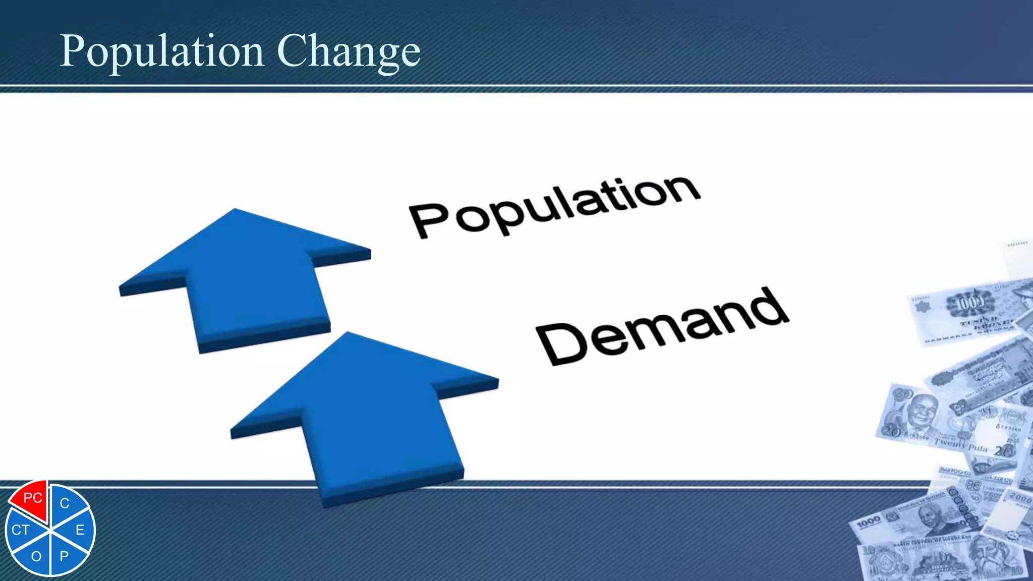
• The direction in which demand would
change depends on the relationships
of products.
C
E
P
O
CT
PC
22.
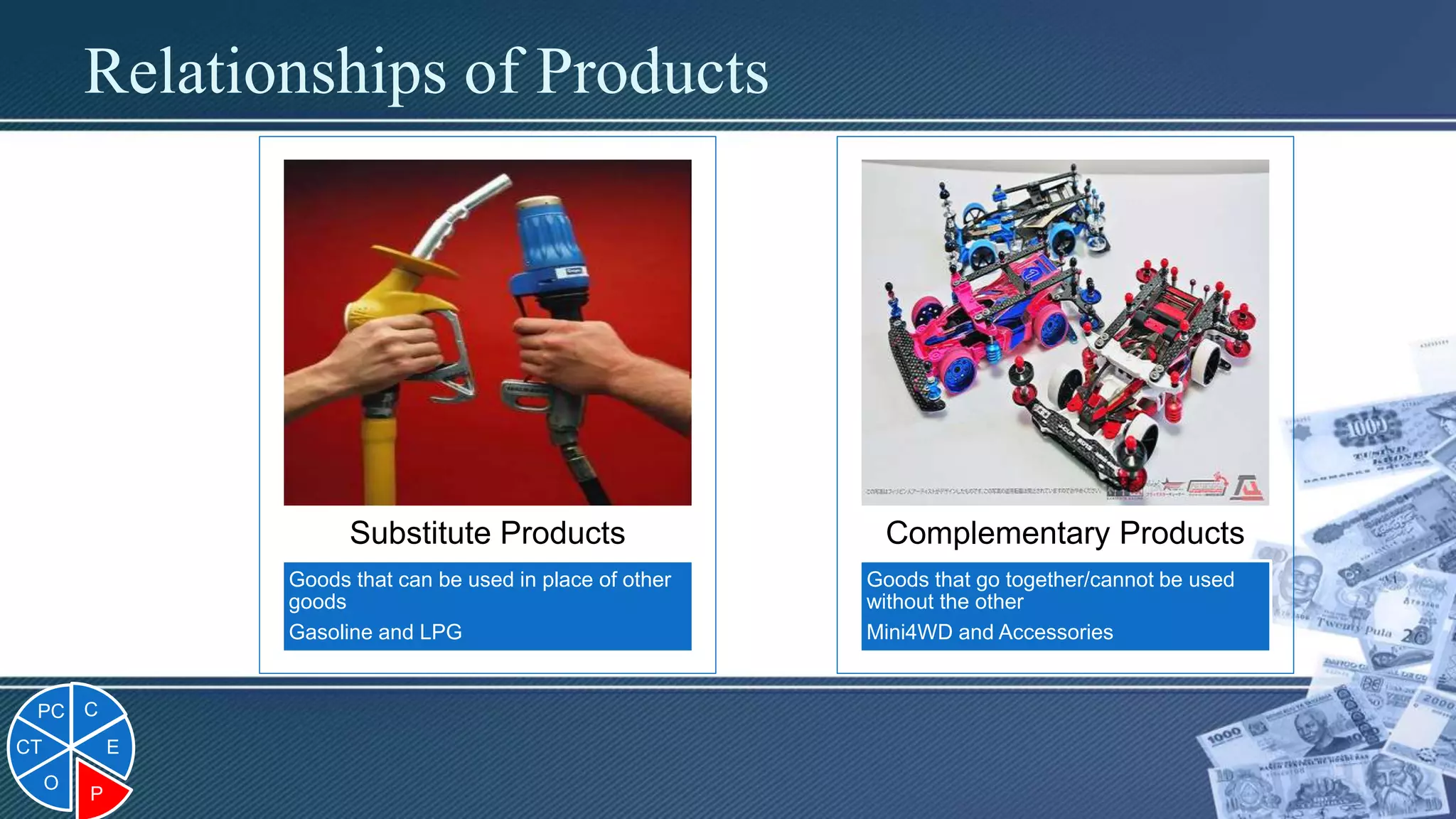
Relationships of Products
Goodsthat can be used in place of other
goods
Gasoline and LPG
Substitute Products
Goods that go together/cannot be used
without the other
Mini4WD and Accessories
Complementary Products
C
E
P
O
CT
PC
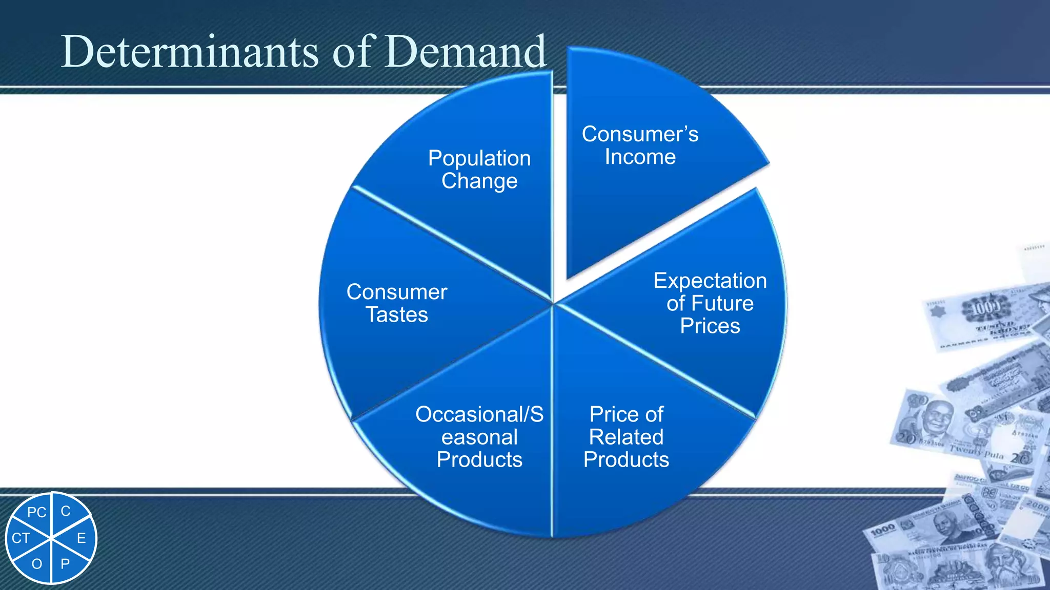
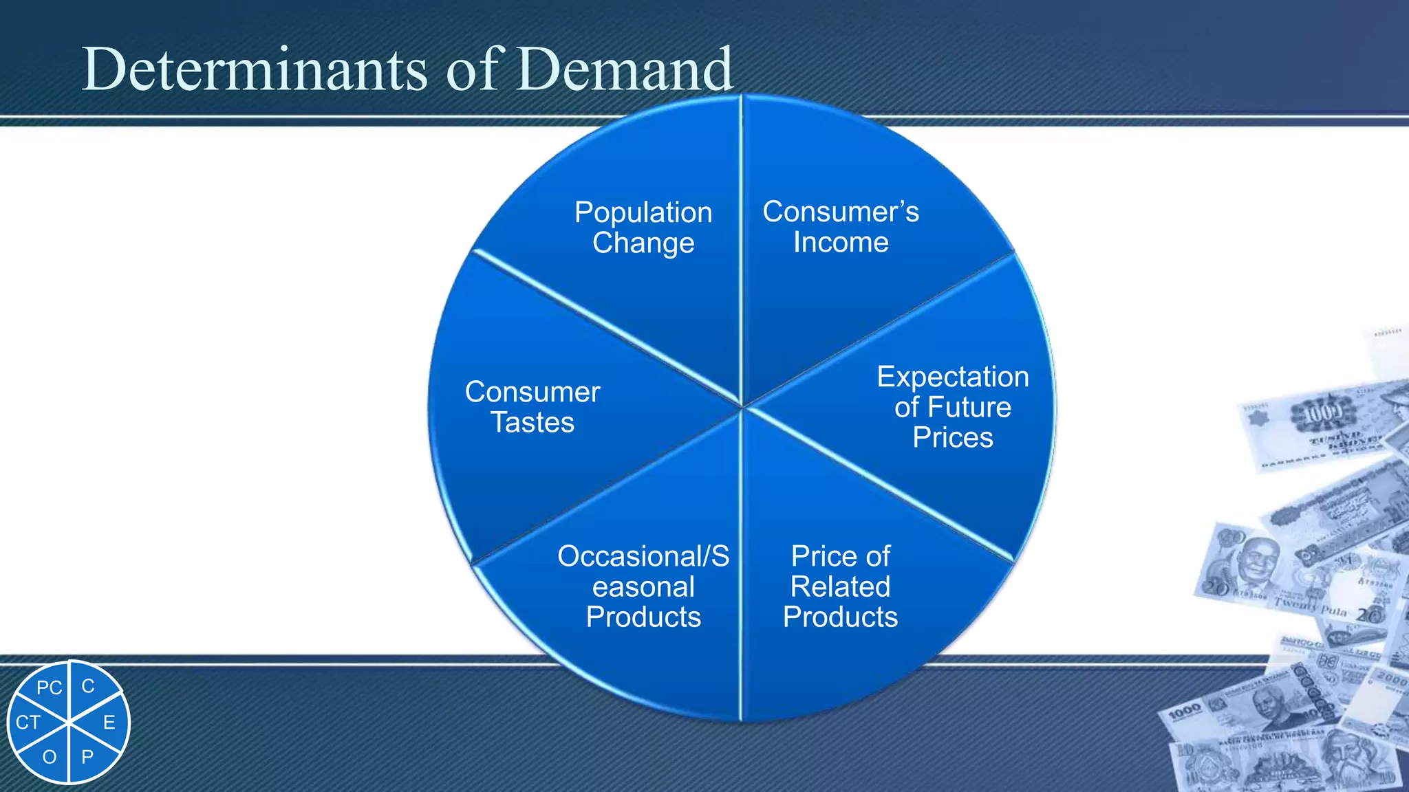
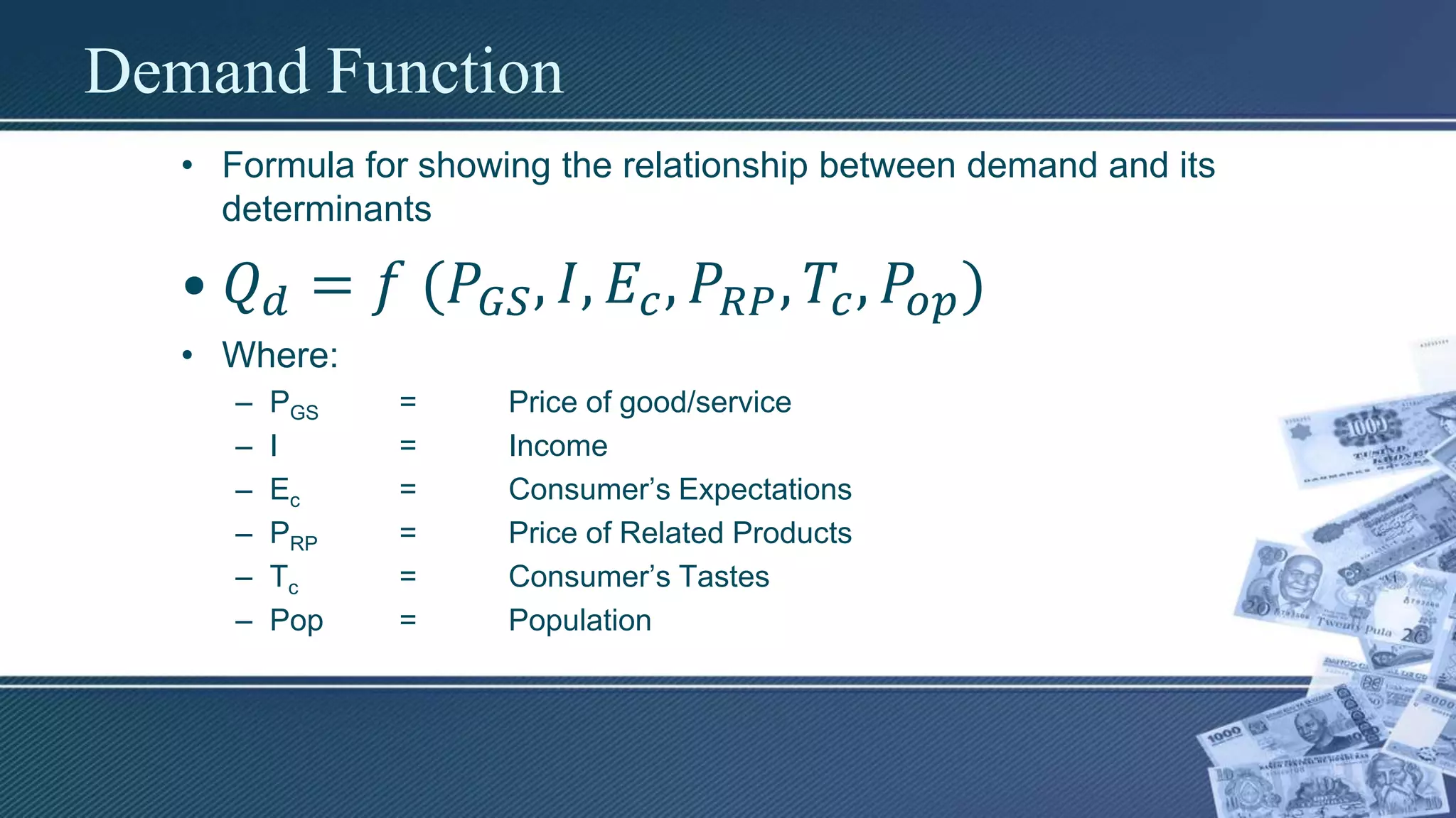
Demand Function
• Formulafor showing the relationship between demand and its
determinants
• 𝑄 𝑑 = 𝑓 (𝑃𝐺𝑆, 𝐼, 𝐸𝑐, 𝑃𝑅𝑃, 𝑇𝑐, 𝑃𝑜𝑝)
• Where:
– PGS = Price of good/service
– I = Income
– Ec = Consumer’s Expectations
– PRP = Price of Related Products
– Tc = Consumer’s Tastes
– Pop = Population
31.
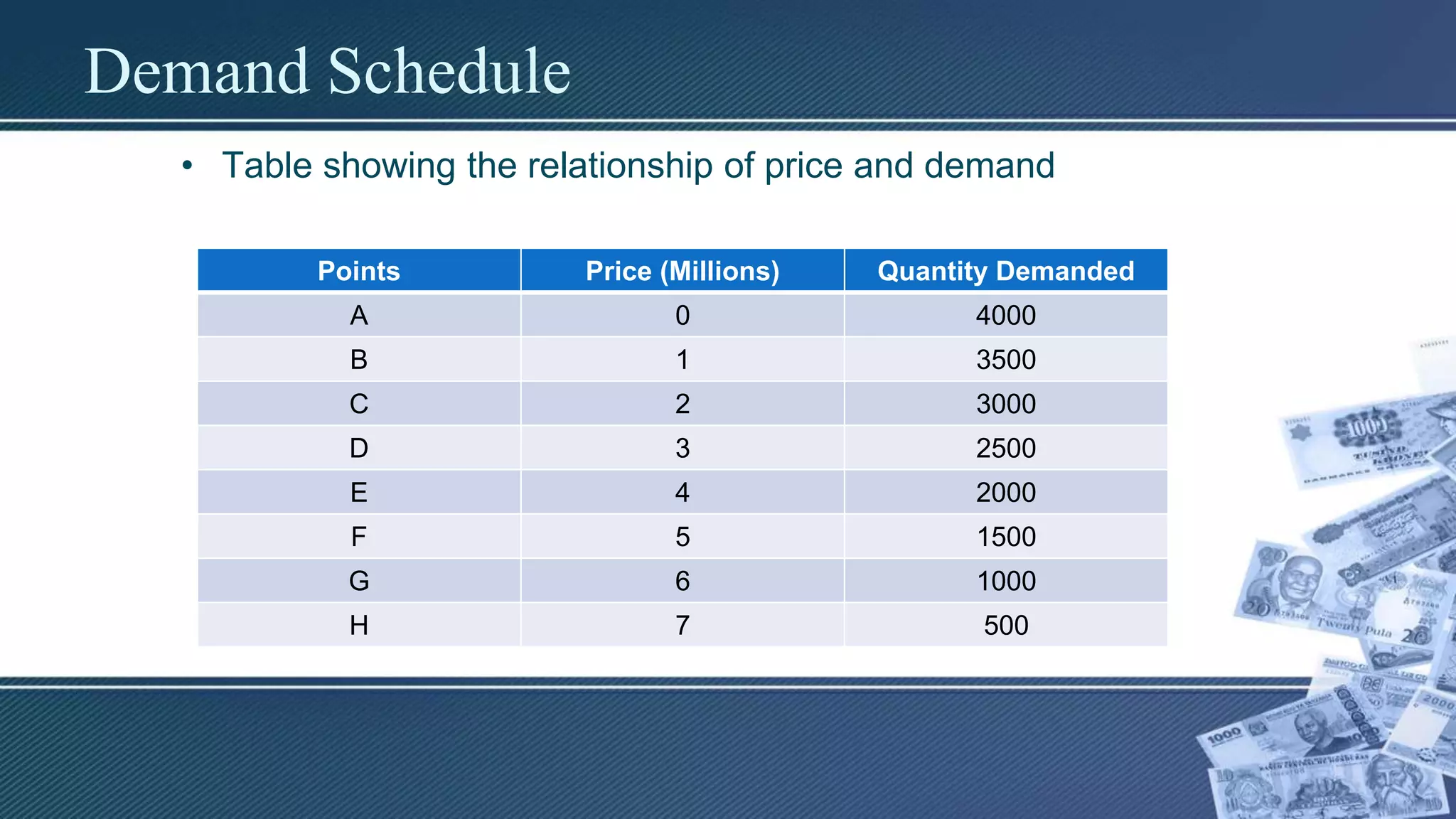
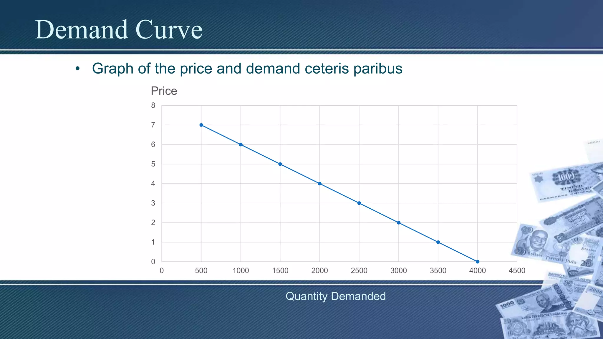
Demand Schedule
• Tableshowing the relationship of price and demand
Points Price (Millions) Quantity Demanded
A 0 4000
B 1 3500
C 2 3000
D 3 2500
E 4 2000
F 5 1500
G 6 1000
H 7 500
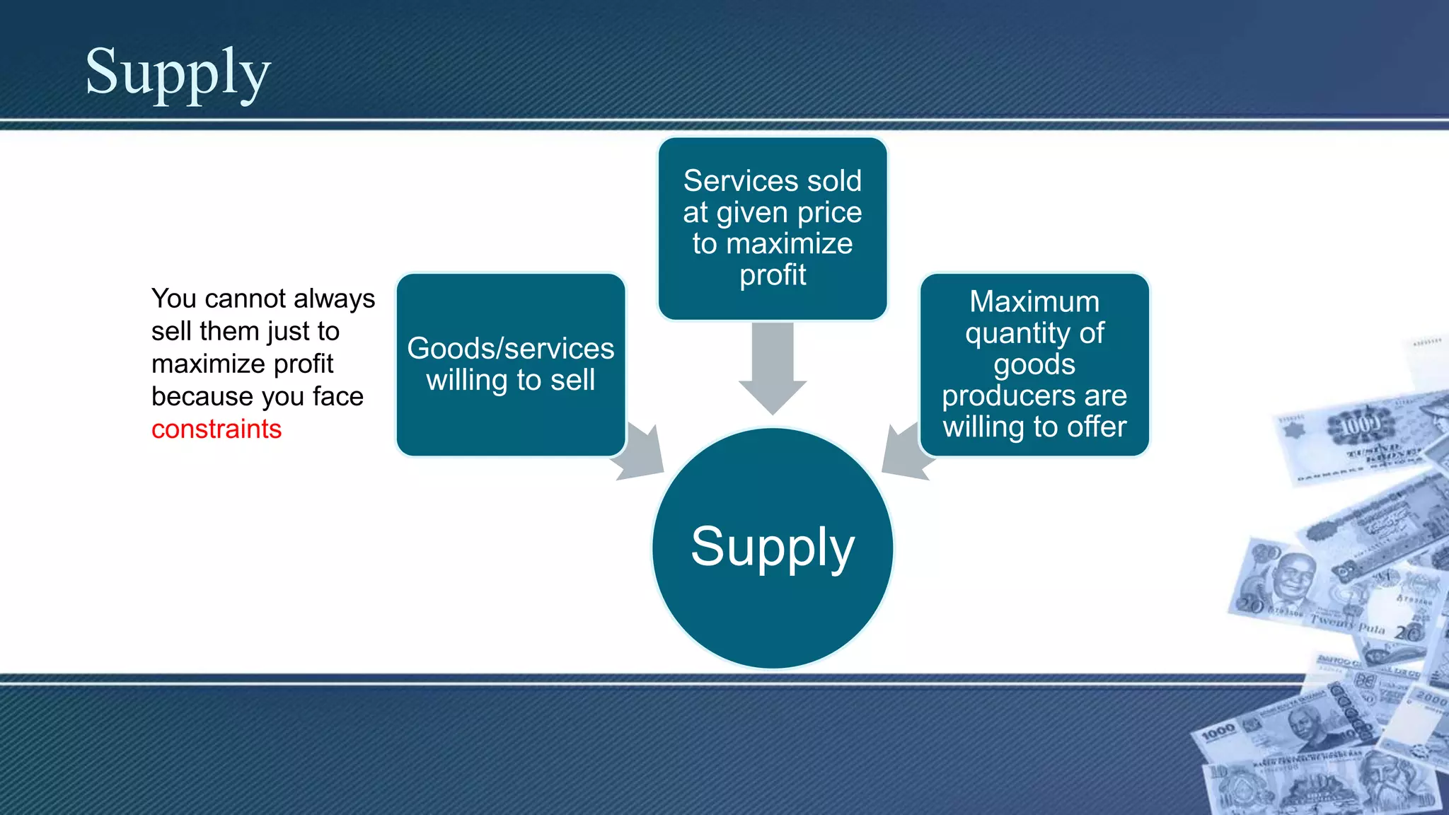
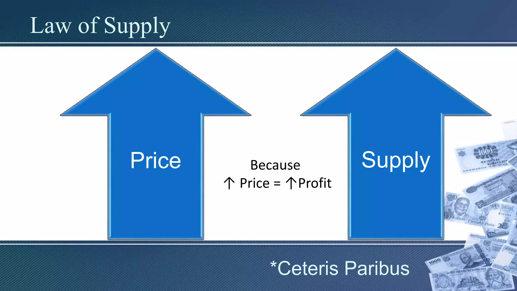
Supply
Supply
Goods/services
willing to sell
Servicessold
at given price
to maximize
profit
Maximum
quantity of
goods
producers are
willing to offer
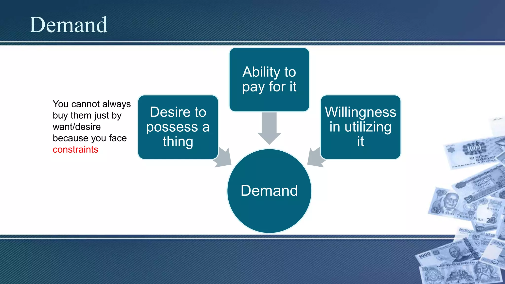
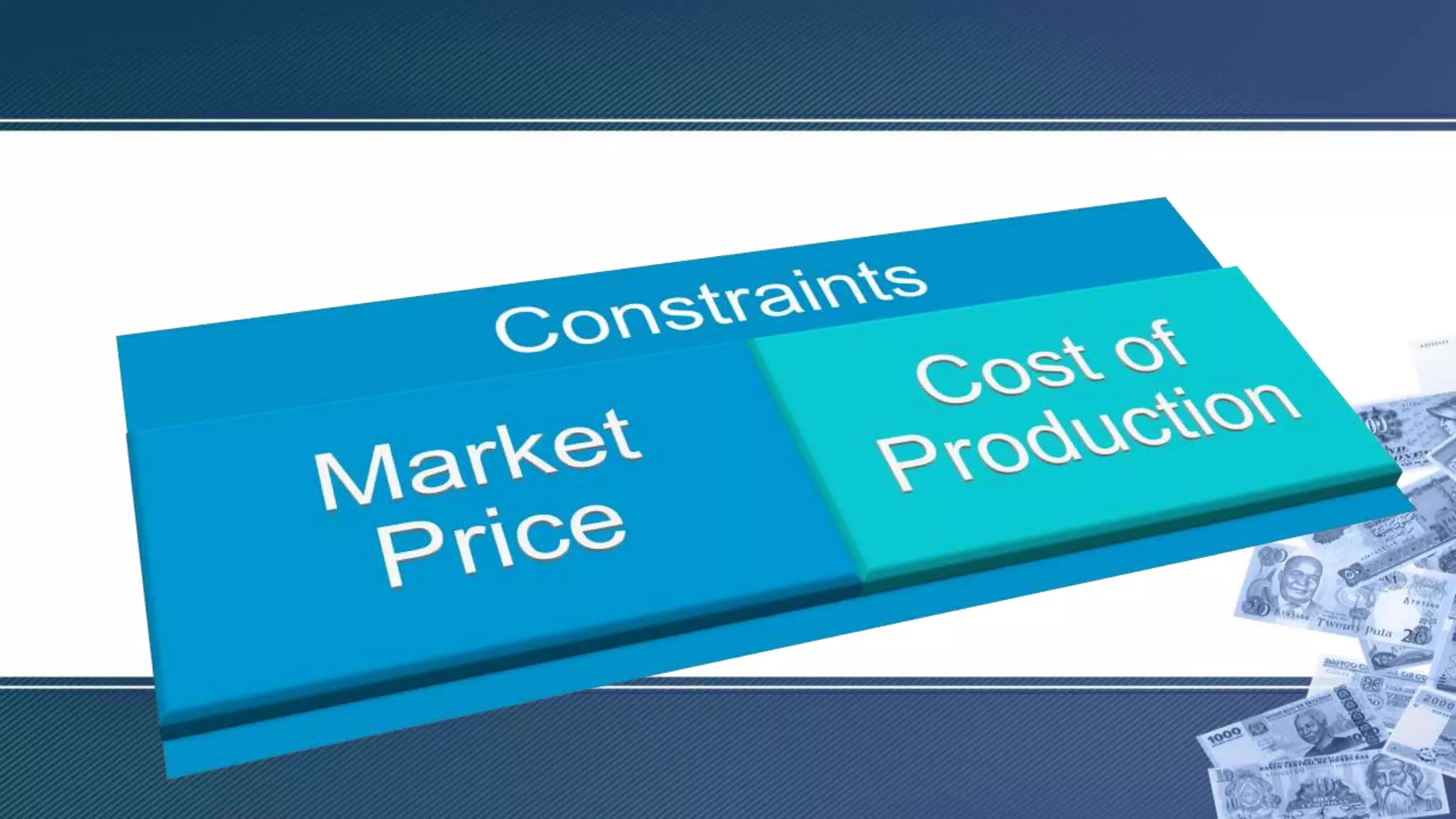
You cannot always
sell them just to
maximize profit
because you face
constraints
36.
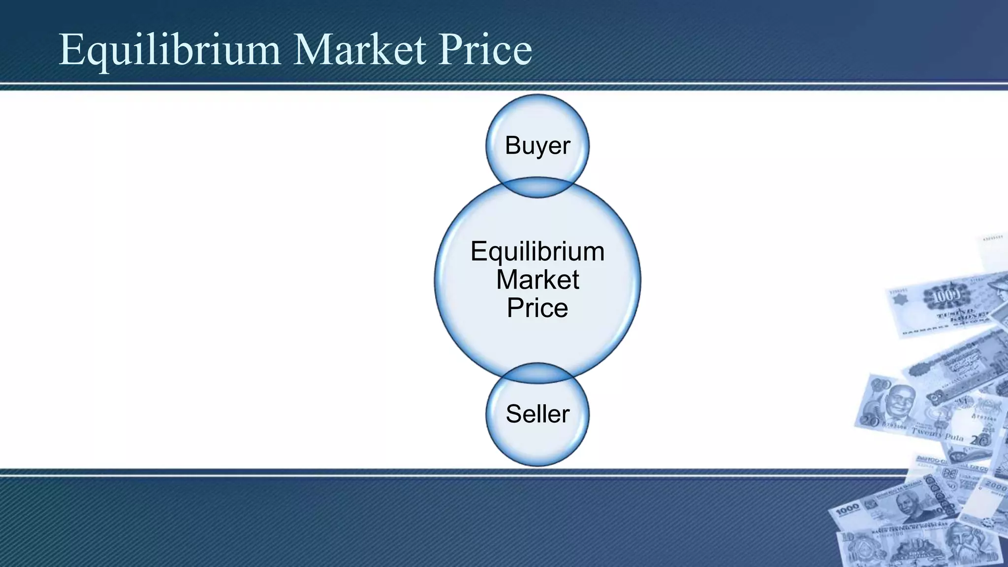
Market Price
• Itis the price that the sellers can
charge their product in a
competitive market.
38.
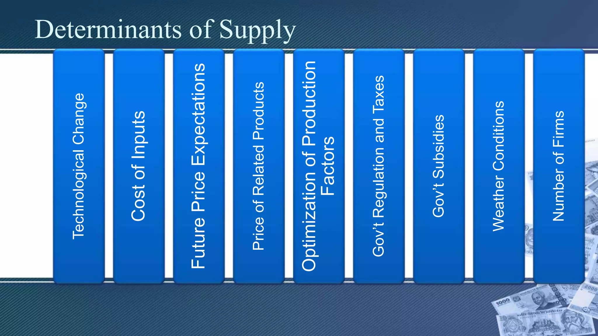
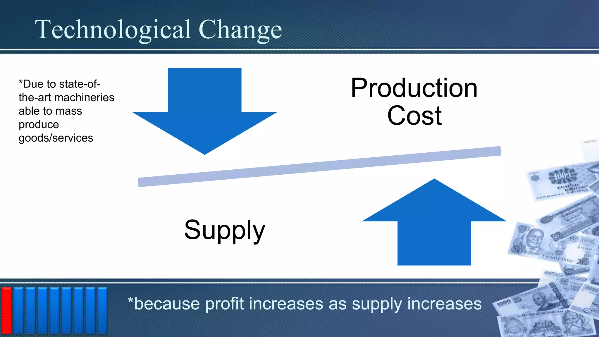
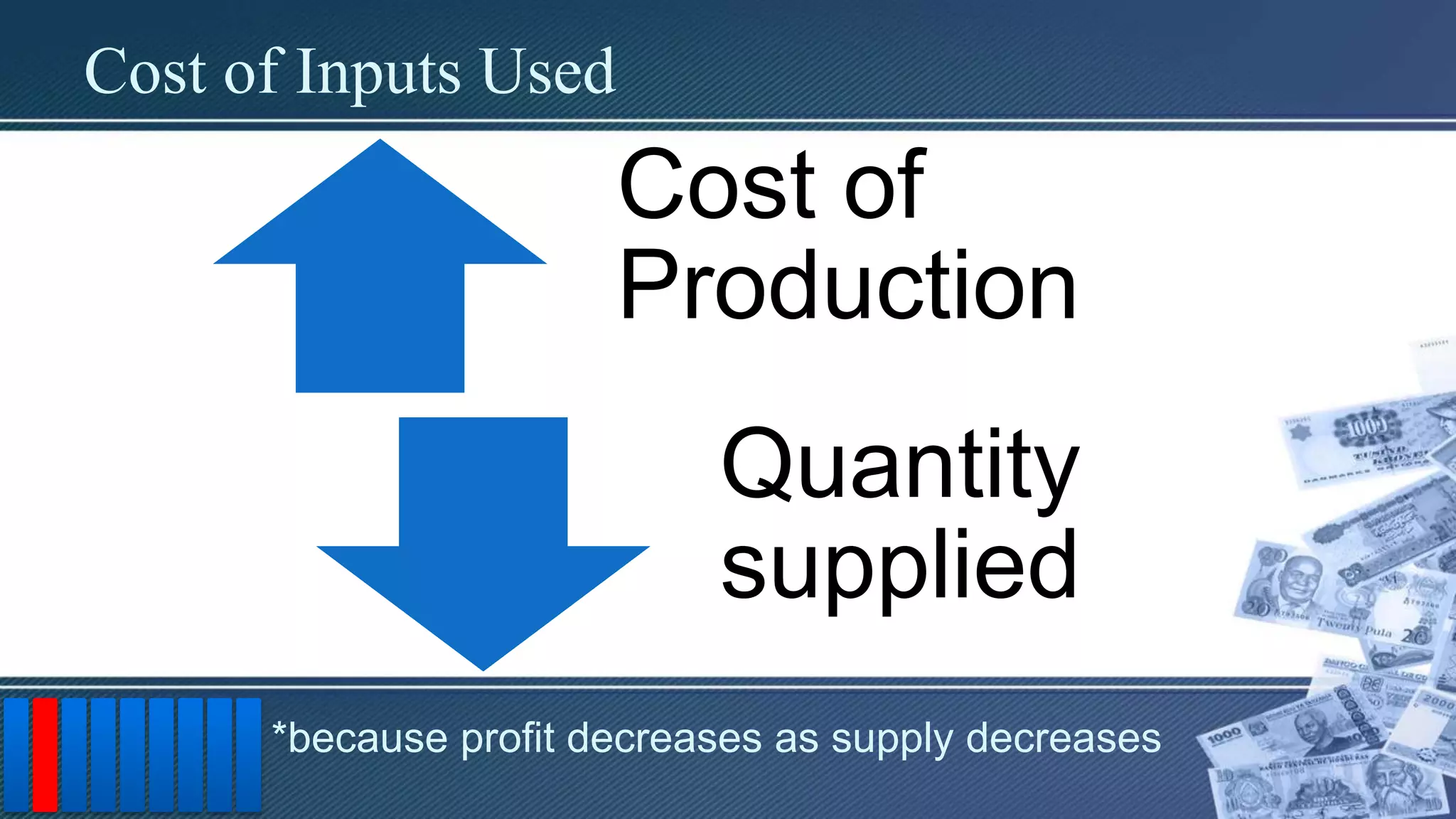
Cost of Production
•The costs of the production
process and the prices of inputs
that they have used to make the
product
Price of RelatedProducts
• Changes in the supply of goods have
significant effect in the supply of such goods.
47.
Optimization of ProductionFactors
• The process/methodology of making
something as fully perfect, functional, or
effective as possible.
• Efficient use of resources
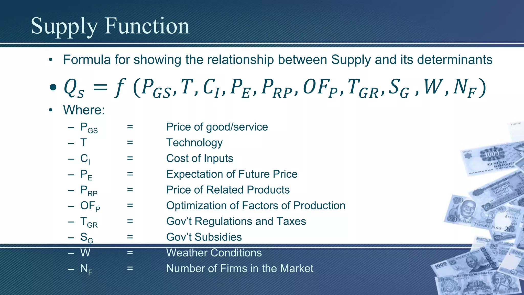
Supply Function
• Formulafor showing the relationship between Supply and its determinants
• 𝑄𝑠 = 𝑓 (𝑃𝐺𝑆, 𝑇, 𝐶𝐼, 𝑃𝐸, 𝑃𝑅𝑃, 𝑂𝐹𝑃, 𝑇𝐺𝑅, 𝑆 𝐺 , 𝑊, 𝑁𝐹)
• Where:
– PGS = Price of good/service
– T = Technology
– CI = Cost of Inputs
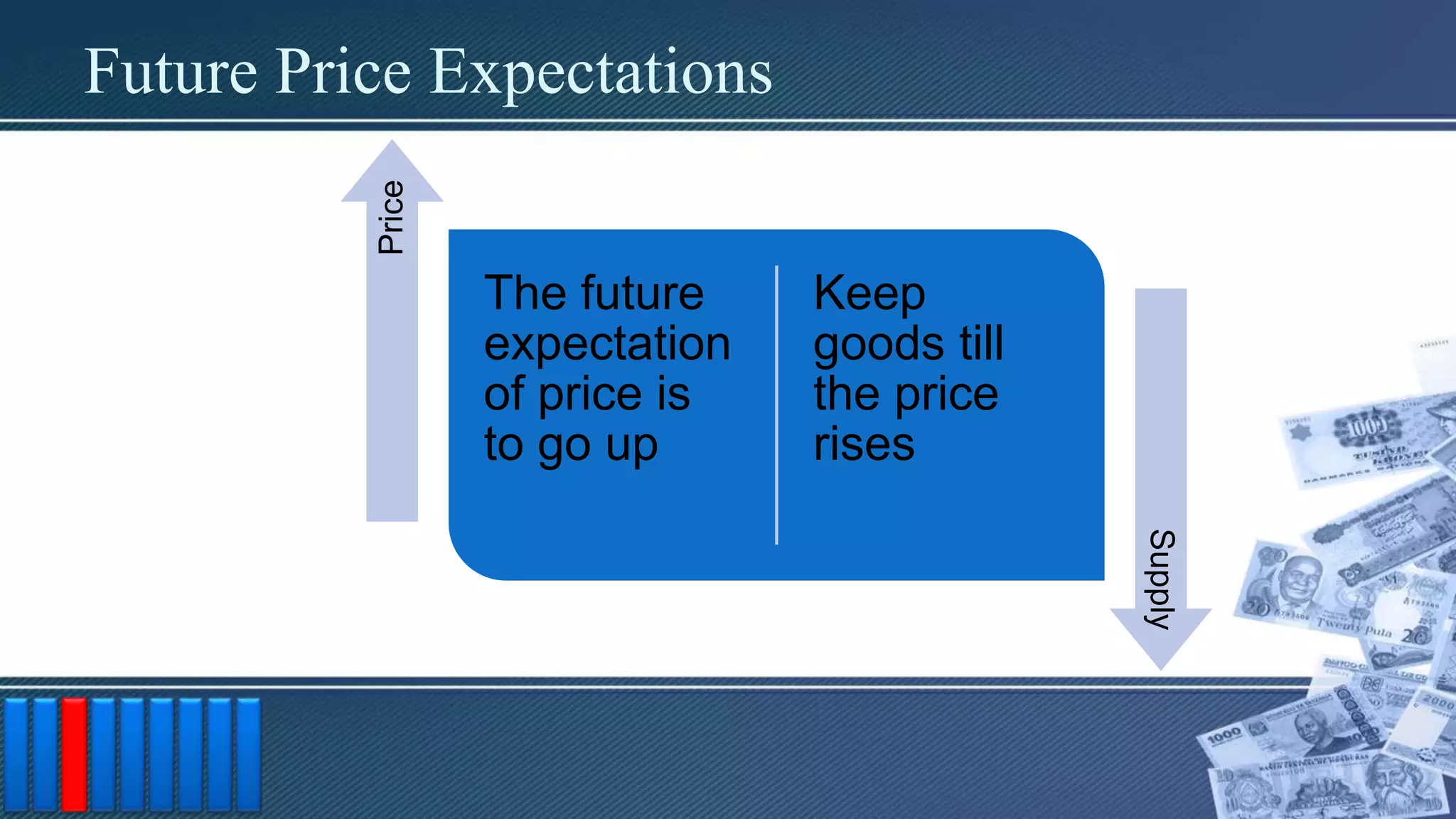
– PE = Expectation of Future Price
– PRP = Price of Related Products
– OFP = Optimization of Factors of Production
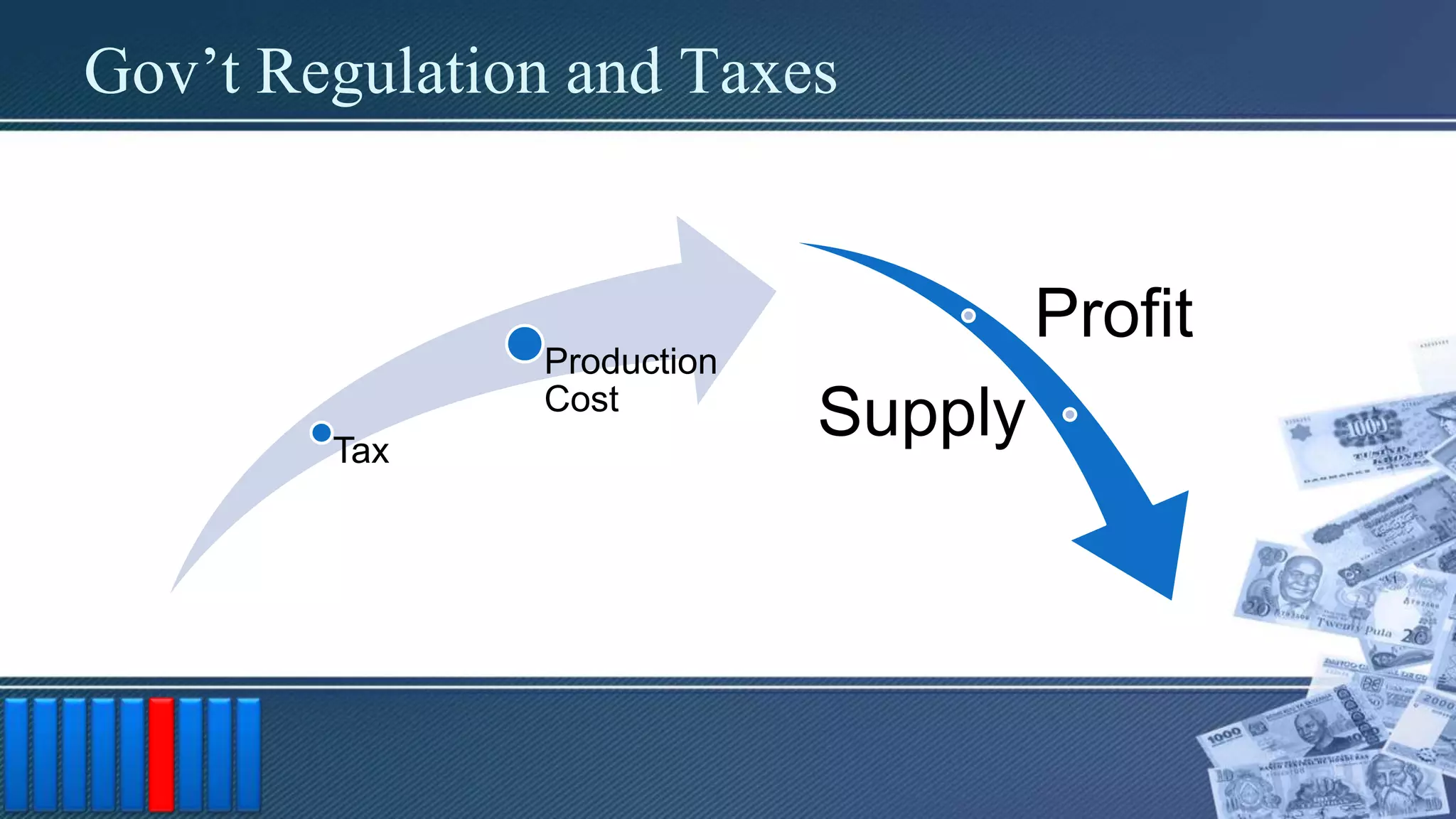
– TGR = Gov’t Regulations and Taxes
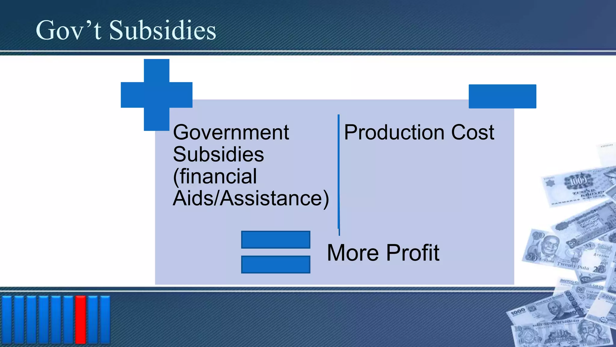
– SG = Gov’t Subsidies
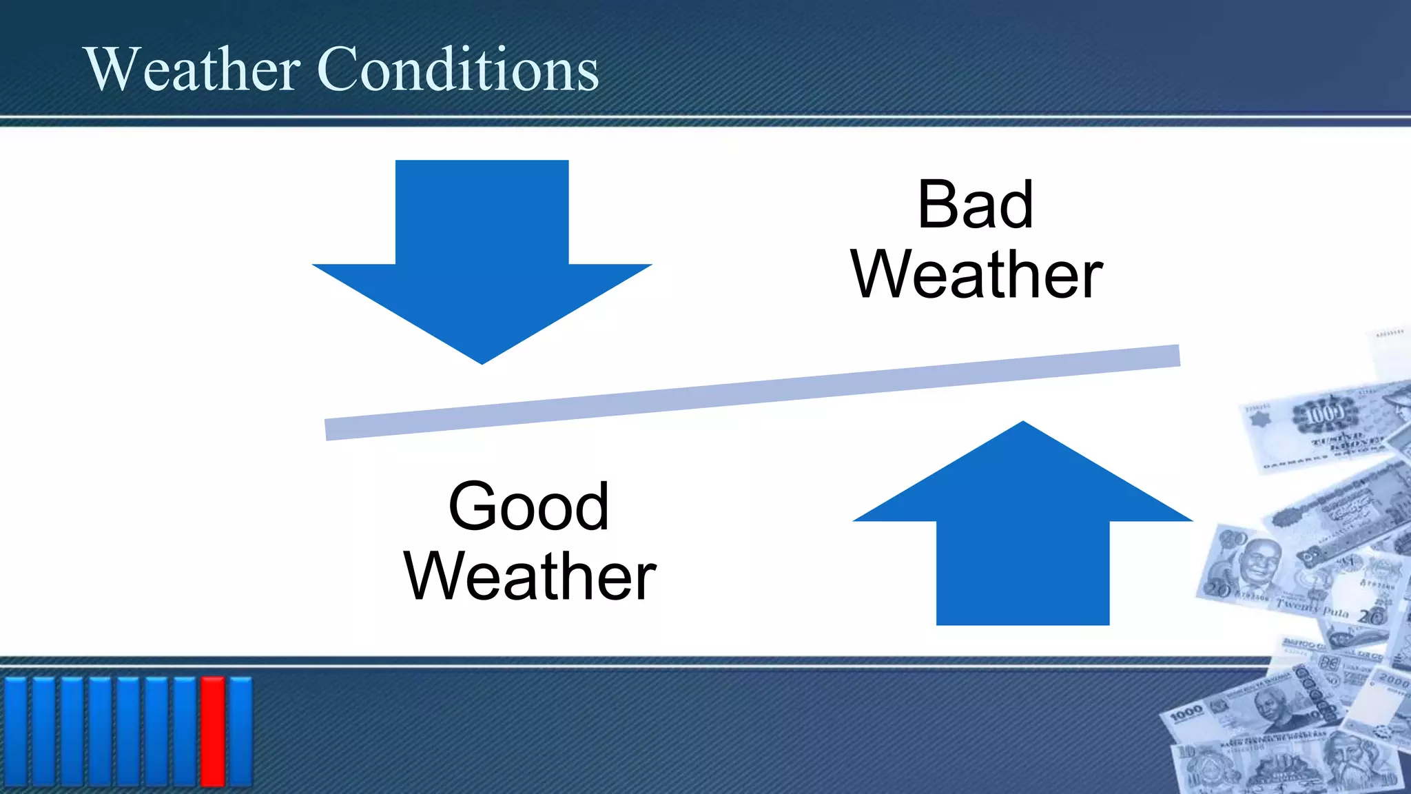
– W = Weather Conditions
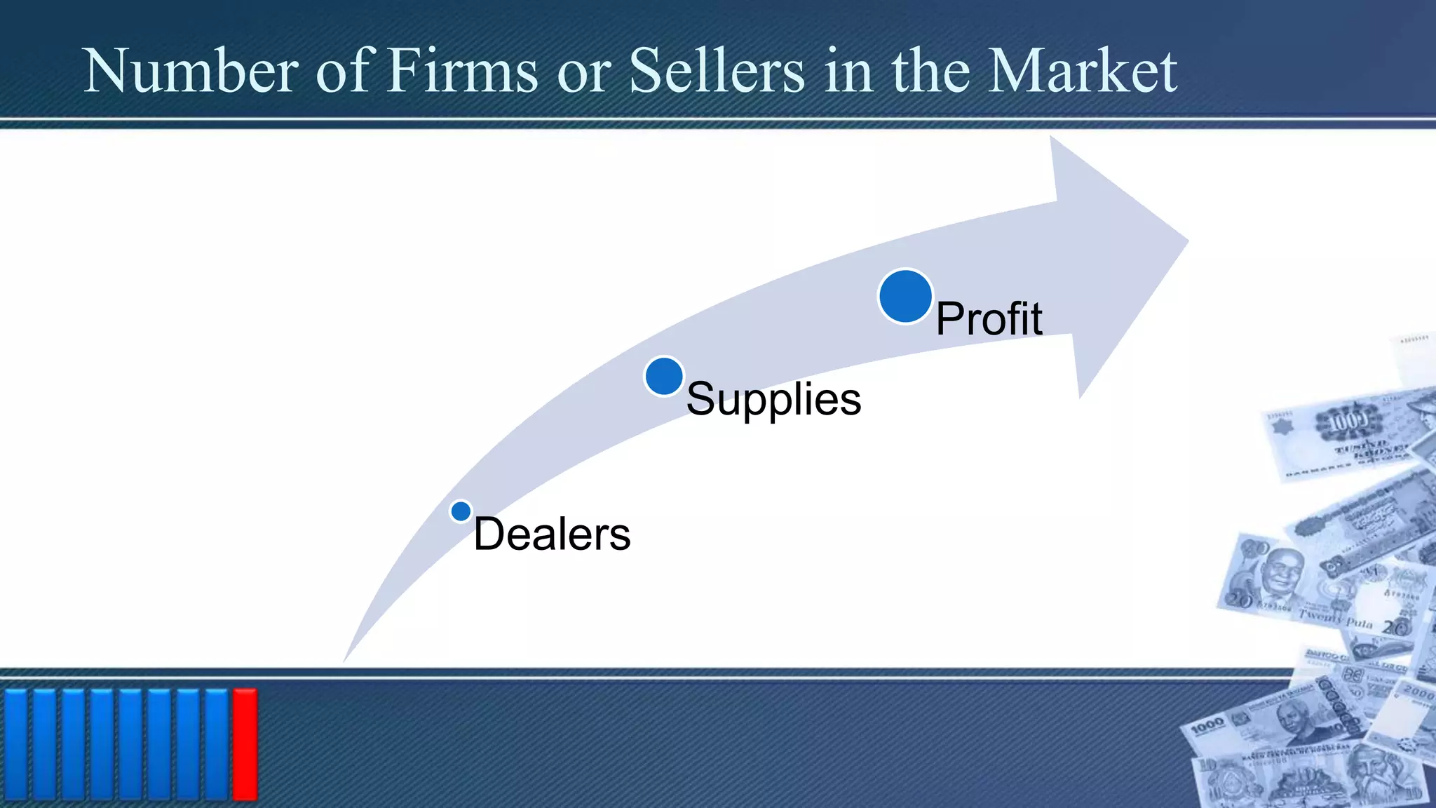
– NF = Number of Firms in the Market
54.
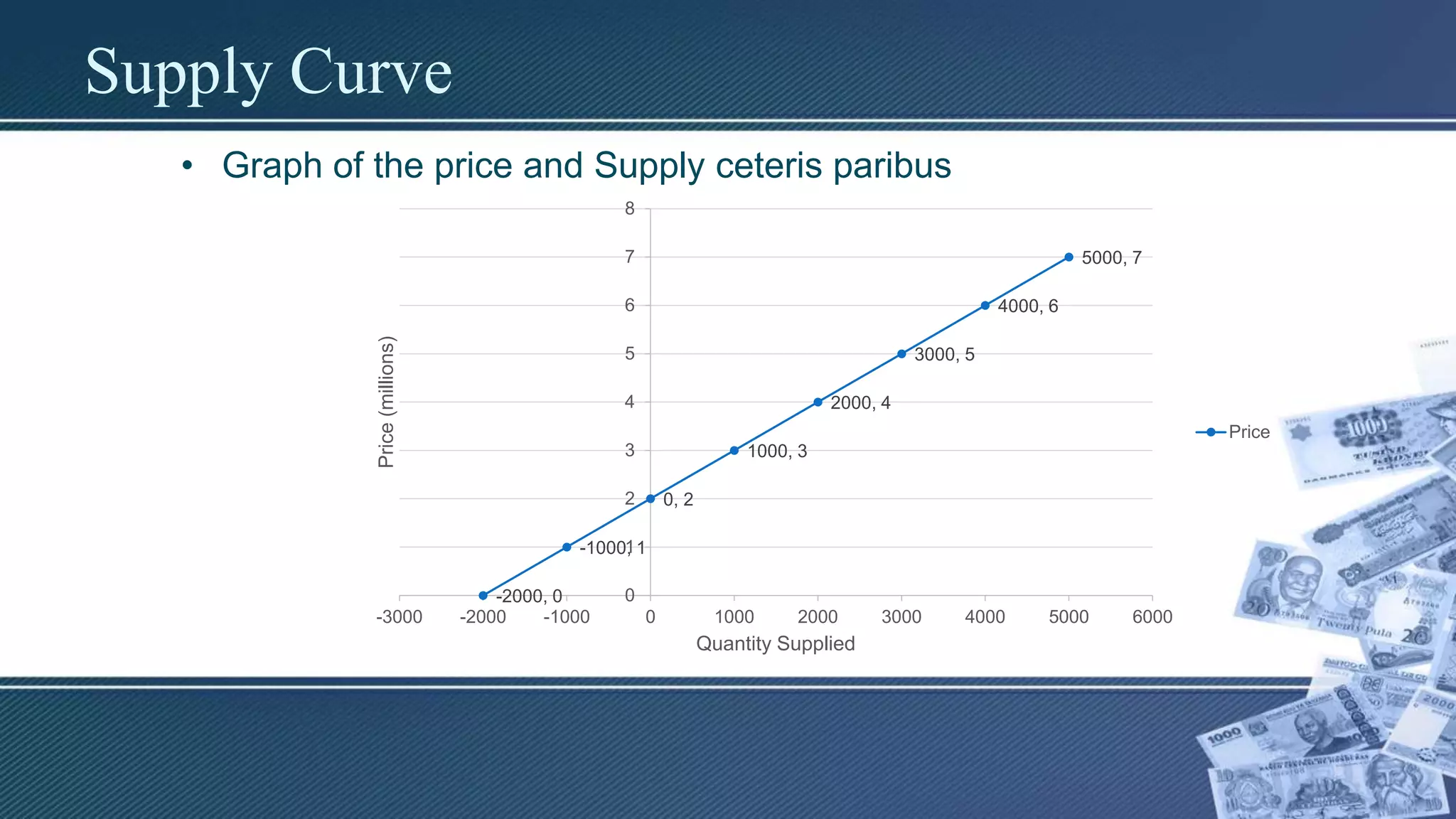
Supply Schedule
• Tableshowing the relationship of Price and Supply
Points Price (Millions) Quantity Supplied
A 0 -2000
B 1 -1000
C 2 0
D 3 1000
E 4 2000
F 5 3000
G 6 4000
H 7 5000
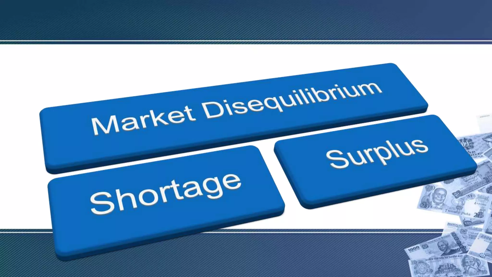
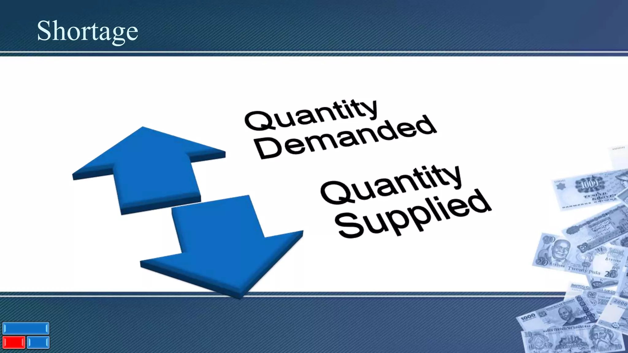
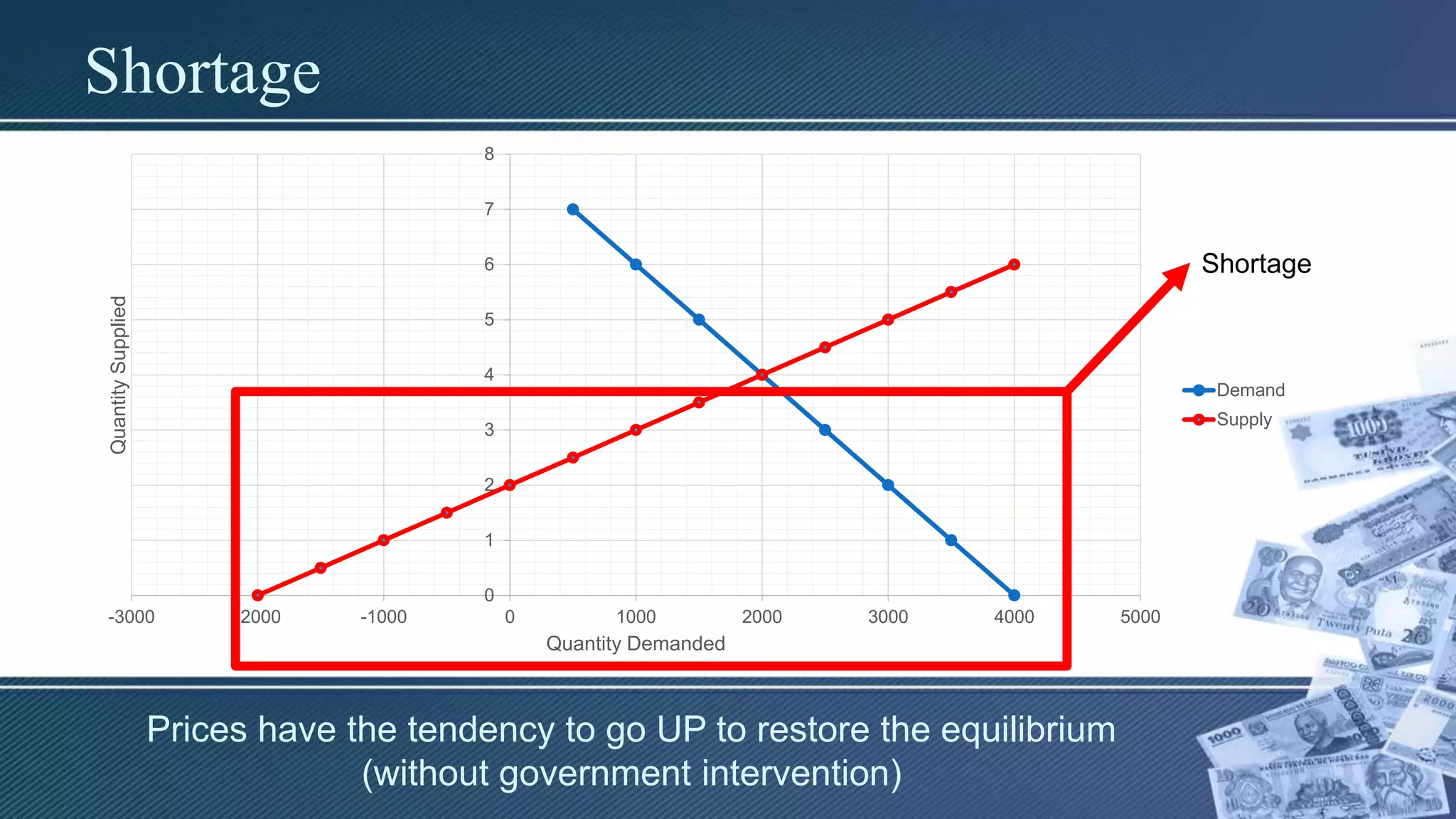
Shortage
0
1
2
3
4
5
6
7
8
-3000 -2000 -10000 1000 2000 3000 4000 5000
QuantitySupplied
Quantity Demanded
Demand
Supply
Shortage
Prices have the tendency to go UP to restore the equilibrium
(without government intervention)
65.
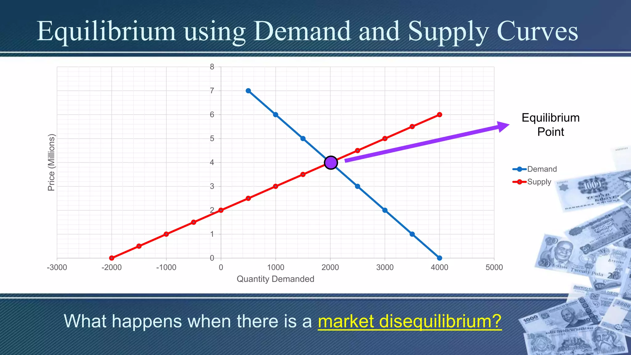
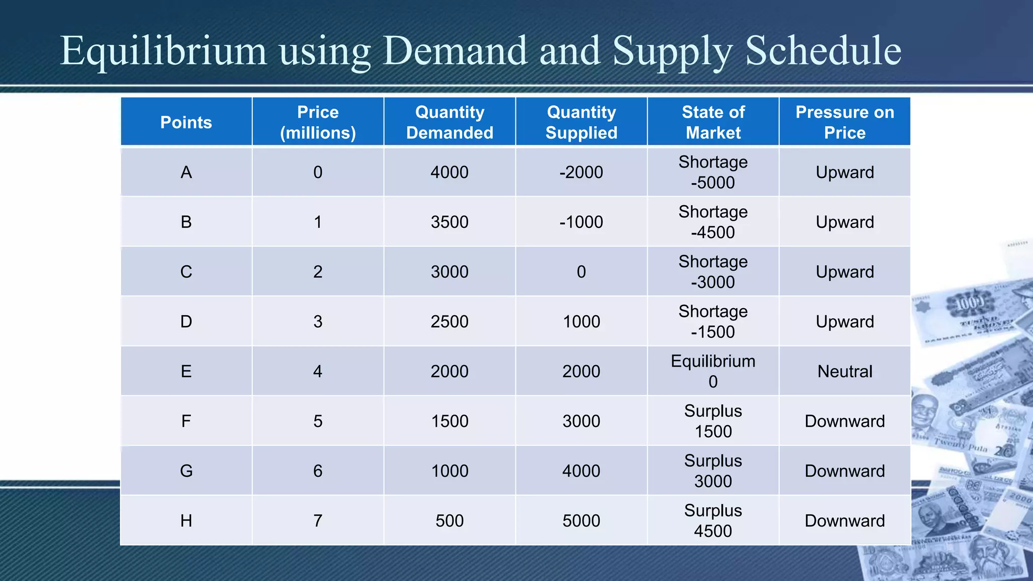
Equilibrium using Demandand Supply Schedule
Points
Price
(millions)
Quantity
Demanded
Quantity
Supplied
State of
Market
Pressure on
Price
A 0 4000 -2000
Shortage
-5000
Upward
B 1 3500 -1000
Shortage
-4500
Upward
C 2 3000 0
Shortage
-3000
Upward
D 3 2500 1000
Shortage
-1500
Upward
E 4 2000 2000
Equilibrium
0
Neutral
F 5 1500 3000
Surplus
1500
Downward
G 6 1000 4000
Surplus
3000
Downward
H 7 500 5000
Surplus
4500
Downward
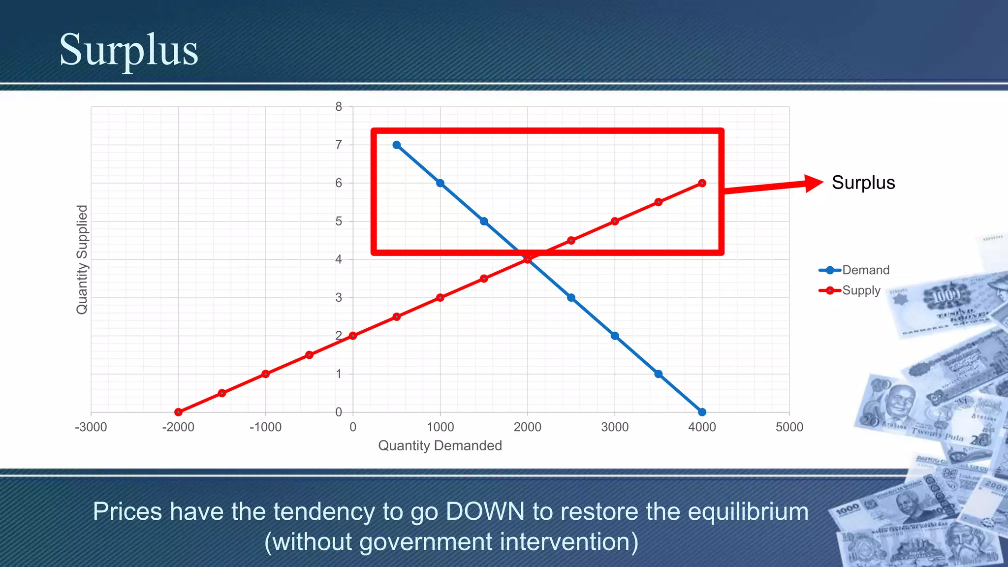
Surplus
0
1
2
3
4
5
6
7
8
-3000 -2000 -10000 1000 2000 3000 4000 5000
QuantitySupplied
Quantity Demanded
Demand
Supply
Surplus
Prices have the tendency to go DOWN to restore the equilibrium
(without government intervention)
69.
Equilibrium using Demandand Supply Schedule
Points
Price
(millions)
Quantity
Demanded
Quantity
Supplied
State of
Market
Pressure on
Price
A 0 4000 -2000
Shortage
-5000
Upward
B 1 3500 -1000
Shortage
-4500
Upward
C 2 3000 0
Shortage
-3000
Upward
D 3 2500 1000
Shortage
-1500
Upward
E 4 2000 2000
Equilibrium
0
Neutral
F 5 1500 3000
Surplus
1500
Downward
G 6 1000 4000
Surplus
3000
Downward
H 7 500 5000
Surplus
4500
Downward
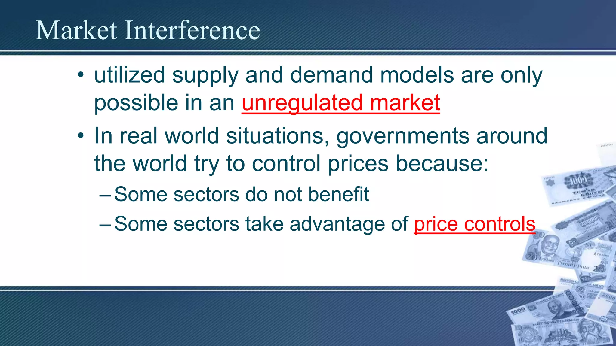
Market Interference
• utilizedsupply and demand models are only
possible in an unregulated market
• In real world situations, governments around
the world try to control prices because:
–Some sectors do not benefit
–Some sectors take advantage of price controls
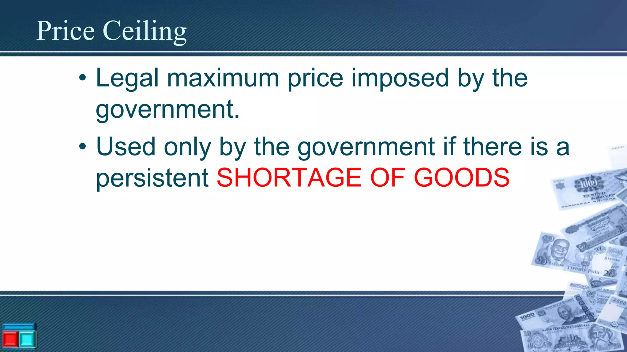
Price Ceiling
• Legalmaximum price imposed by the
government.
• Used only by the government if there is a
persistent SHORTAGE OF GOODS
75.
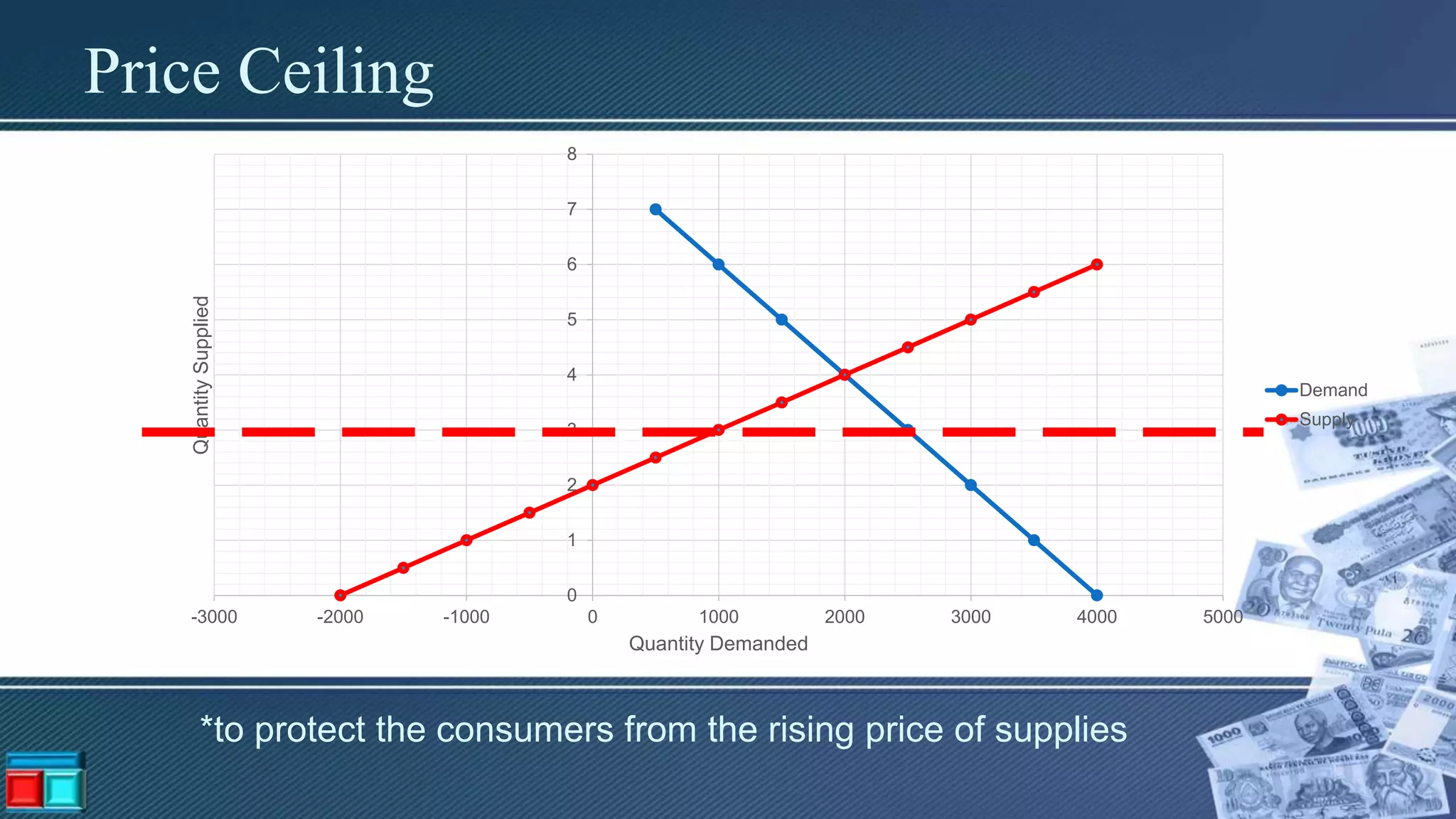
Price Ceiling
0
1
2
3
4
5
6
7
8
-3000 -2000-1000 0 1000 2000 3000 4000 5000
QuantitySupplied
Quantity Demanded
Demand
Supply
*to protect the consumers from the rising price of supplies
77.
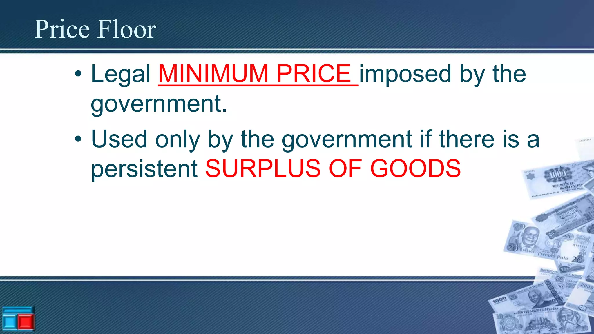
Price Floor
• LegalMINIMUM PRICE imposed by the
government.
• Used only by the government if there is a
persistent SURPLUS OF GOODS
78.
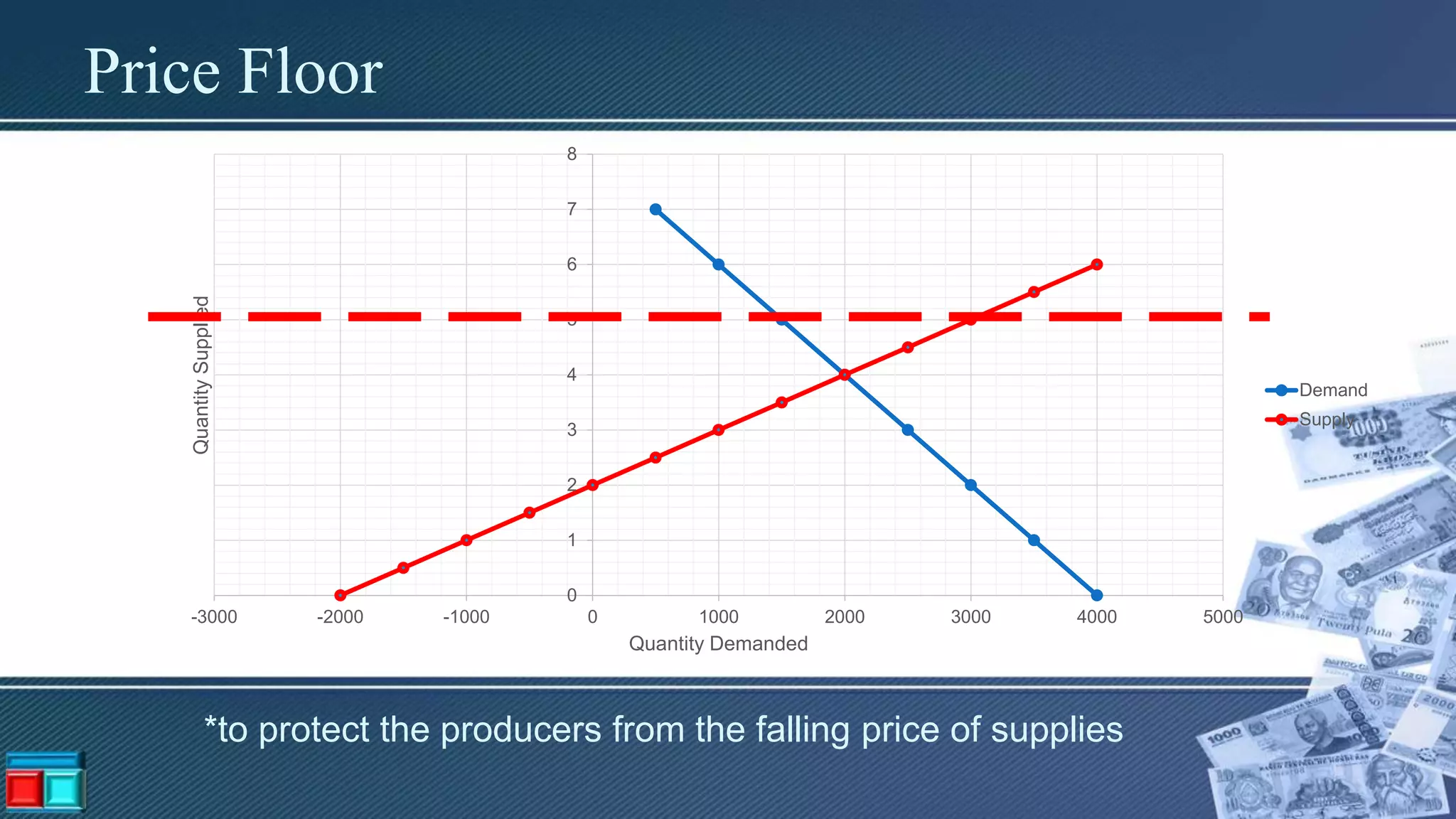
Price Floor
0
1
2
3
4
5
6
7
8
-3000 -2000-1000 0 1000 2000 3000 4000 5000
QuantitySupplied
Quantity Demanded
Demand
Supply
*to protect the producers from the falling price of supplies
79.
Humans and animalsare both selfish. They virtually don’t
care about others. They say clever things, make relationships
where both sides use each other, and look for a way to profit
themselves while limiting the loss for the other group.