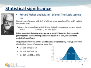
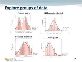
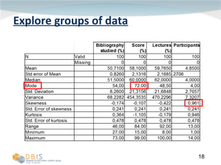
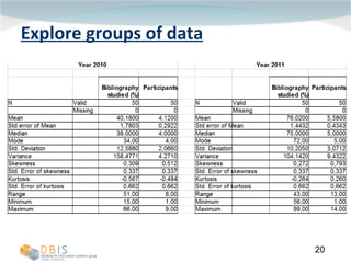
This document discusses exploring and representing data properties through statistical analysis techniques. It covers topics like descriptive statistics, graphical representations of data through histograms and boxplots, testing for normality and homogeneity of variance, and exploring differences between groups of data. The goal is to properly examine data distributions and assumptions before conducting further statistical tests and analysis.

1. Back to the basics, Part2
Data exploration:
representing and testing data properties
Spyros Veronikis
Electrical and Electronics Engineer
Dept. of Archives and Library Sciences
Ionian University
spver@ionio.gr
http://dlib.ionio.gr/~spver/seminars/statistics/
More information

2. Seminar Content
 Basic statistics concepts
 Data exploration
 Correlation
 Comparing two means
 Comparing several means (ANOVA)
 Non-parametric test
 Nominal data
2

3. Today's Content
 Statistical significance
 Parametric Data
 Histograms and Boxplots
 Descriptive statistics
 Correcting problems in the data
 Exploring groups of data
 Testing whether a distribution is normal
 Testing for homogeneity of variance
 Summary
3

4. Statistical significance
 Ronald Fisher and Muriel Bristol, The Lady tasting
tea
Given 6 cups of tea and milk (in 3 of which the tea was placed first and 3 had the
milk added first)
“What is the probability that lady Bristol finds all 3 cups where tea was placed
first?” (Answer: 1/20= 0.05 ή 5%)
Fisher suggested that only when we are at least 95% certain that a result is
genuine (not a chance finding) should we accept it as true, and therefore
statistically significant.
Frequency distributions can be used to assess the probability. In a typical normal
distribution, chance of z occuring more than:

Z= 1.96 is 0.05 or 5%

Z= 2.58 is 0.01 or 1%

Z= 3.29 is 0.001 or 0,1%
4

5. Parametric data
 Assumptions of parametric tests:
1. Normally distributed data:

Checked with histograms and Kolmogorov-Smirnov or Shapiro-Wilk criterion
2. Homogeneity of variance

In several groups: data in samples come from populations of same variance

In correlational designs: variance of one variable remains stable across all levels of
other variable(s)
3. Interval data

Arithmetic values, equal differences among successive points in measurement scale
4. Independence

Data come from different participants who don't influence each other.
Only requirements 1 and 2 are tested by objective criteria (tests). Requirements 3 and 4 are
tested by common sense.
5

6. Graphing and screening data
 Histograms
 Show the number of
times each recorded
value occurs
 The horizontal axis
represents the levels of
measurement of the
variable
 They make outliers easy
to spot
6

7. Outliers
 These are scores very different from the rest of the data
 They occur rarely
 They can bias the model we fit to the data
 They need to be identified and omitted from the dataset
7

8. Graphing and screening data
 Boxplots (box-whisker diagrams)
– Show the lowest and highest scores
– Show the quartile (25%) ranges
– Show the interquartile range (50%)
– Show the median*
 Normal distribution has a symmetrical
boxplot
 Skewed distributions don't
 Platykurtic distributions have wide
boxplots
* The median of a list of numbers is the number that splits the dataset in half.
E.g. for dataset A={1,2,2,4,13,15,51} the median is 4 (the average is 12.57)
8

9. Graphing and screening data
9

10. Descriptive statistics
 “An alternative search tool was provided to the library patrons and
we assess its adoption by recording the number of hours spent on
the previous tool before and after 2 demonstration sessions”.
 Descriptive statistics
 Mean, Standard error of mean
 Median
 Mode
 Standard deviation
 Variance
 Skewness and std. Error
 Kurtosis and std. Error
 Range
 Min, Max
10

11. Descriptive statistics
First Period Second Period Third Period
11

12. Skewness and kurtosis
 These are 0 for normal distribution
 z-values are more informative because they are
standardized
– Skewness: zsk= SK/SEsk
– Kurtosis: zkur= KUR/SEkur
1st period: zsk= -.004/.086= .047, zkur= -2.38
2nd period: zsk= 1.095/.150= 7.30, zkur= -2.75
3rd period: zsk= 1.033/.218= 4.73, zkur= 1.69
12

13. Correcting problems in data
 How do we deal with problems in data (problems in
distribution, outliers, missing values)
– Remove problematic cases
– Transform the data (X → Y= function(X))
 Transformations can correct distribution form, i.e.,
remove skewness by “smoothening” outliers
 Transform ALL data, of ALL variables that are going to be
compared/related even if there are variables that aren't
skewed. This isn't cheating!
 Do the statistic tests and analysis
13

14. Correcting positively skewed data
 Log transformation, Xtr → Log(X):
– Reduces positive skew.
– X must be greater than 0 (shifting might be needed)
 Square root transformation, Xtr → sqrt(X)
– Brings large scores closer to the center
– X must be greater than 0 (shifting might be needed)
 Reciprocal transformation, Xtr → 1/X
– Reduces the impact of large scores
– Reverses the scale. Therefore, prior to transformation we need to
reverse scores ourselves (e.g. Xrev ← HighestX – X). Then X tr →
1 /Xrev
 For negatively skewed data, reverse the scores prior to the above
transformations.
14

15. Transformed data
15

16. Explore groups of data
Example:
 A professor is recording the score of a project report delivered by
his students. He also takes a note to:
– The percentage of the given bibliography studied (biblio)
– Their attendaces in the lectures (lectures)
– The number of student collaborated to deliver the report
(participants).
 He collects the same data a year later (from the students of the
new class) and looks for differences in performance.
 Score= function(biblio, lectures, participants, year)
16

17. Explore groups of data
Project score Bibliography studied
Lectures attended Participants
17

18. Explore groups of data
18

19. Explore groups of data
Comments on overall descriptives (previous table):
 The distribution of score for both years seems bimodal (could be a
difference in performance by year)
 We can compare scores of two years (because each one comes
from a normal distribution), but we can compare the whole dataset
of scores to another similar dataset.
 The participants' distribution might also be due to different
collaborations among years.
 We ask for descriptives per year
19

20. Explore groups of data
20

21. Testing normality of a distribution
 Normality is not assessed visually (i.e., it looks normal to me)
 We mathematically examine whether a given distribution as a whole
deviates from a comparable normal distribution (having same mean
and same standard deviation) .
 We use Kolmogorov-Smirnov and Shapiro-Wilk tests
“Is the given distribution different than normal?”
 None significant test outcome (p>. 05) indicates similar distribution,
therefore normality
 A difference (outcome) found significant (p< 0.05) shows non-
normality
21

22. Testing for homogeneity of variance
 Homogeneity of variance is a requirement for parametric tests to
be applied
 As you go through the levels of one variable, the variance of
another variable must not change
“For how many hours do you feel sick after an extra pint of beer?”
22

23. Testing for homogeneity of variance
 For groups of data we use Levene's test which reveals if there is homogeneity of
variance.
 It test the hypothesis that “There is no difference between variances in the
groups”, i.e., the difference between variances is zero.
– If the test outcome (difference) is found significantly different from 0
(i.e., there is a difference and that is not a chance finding, p<.05) then
we reject the null hypothesis and acknowledge heterogeneous
variances.
– If the test outcome is found non-significant (error probability p>.05) then
we accept the null hypothesis and consider the group data to be of
homogeneous variance.
Levene df1 df2 Significance
statistic (d)
Score 2.584 1 98 0.111 > 0.05
Participants 7.368 1 98 0.008 < 0.05
23

24. Summary
 What we 've seen
 Examine data properly before proceeding to
analysis
 Look at the data distribution
 Spot any problems (e.g. outliers)
 In case of non-normality try to transform data
 When comparing data from different groups look
at distributions within each group
 Also test for homogeneity of variance
24

25. References
 Field, A. (2005). Discovering Statistics Using SPSS,
2nd ed., Sage Publications.
 Statsoft, Inc. (2011). Electronic Statistics Textbook.
Tulsa, OK: Statsoft. WEB:
http://www.statsoft.com/textbook/
25