Data Analytics notes

1. Data Analytics-Introduction
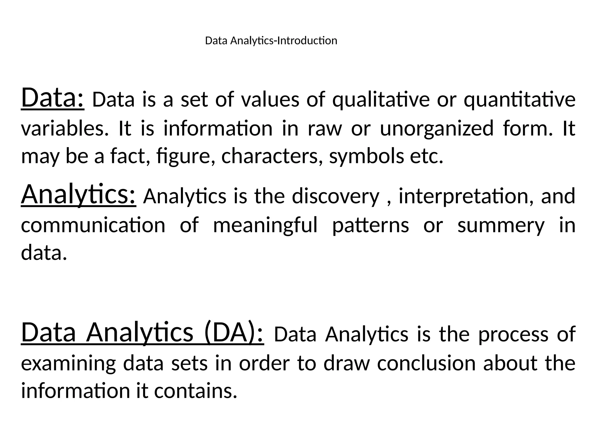
Data: Data is a set of values of qualitative or quantitative
variables. It is information in raw or unorganized form. It
may be a fact, figure, characters, symbols etc.
Analytics: Analytics is the discovery , interpretation, and
communication of meaningful patterns or summery in
data.
Data Analytics (DA): Data Analytics is the process of
examining data sets in order to draw conclusion about the
information it contains.

2. Types of analytics
1] Descriptive Analytics : “What has happened?”
(Data aggregation, summary, data mining)
2] Predictive Analytics : “What might happen?”
(Regression, LSE,MLE)
3] Prescriptive Analytics : “What should we do?”
(Optimization, Recommendation)

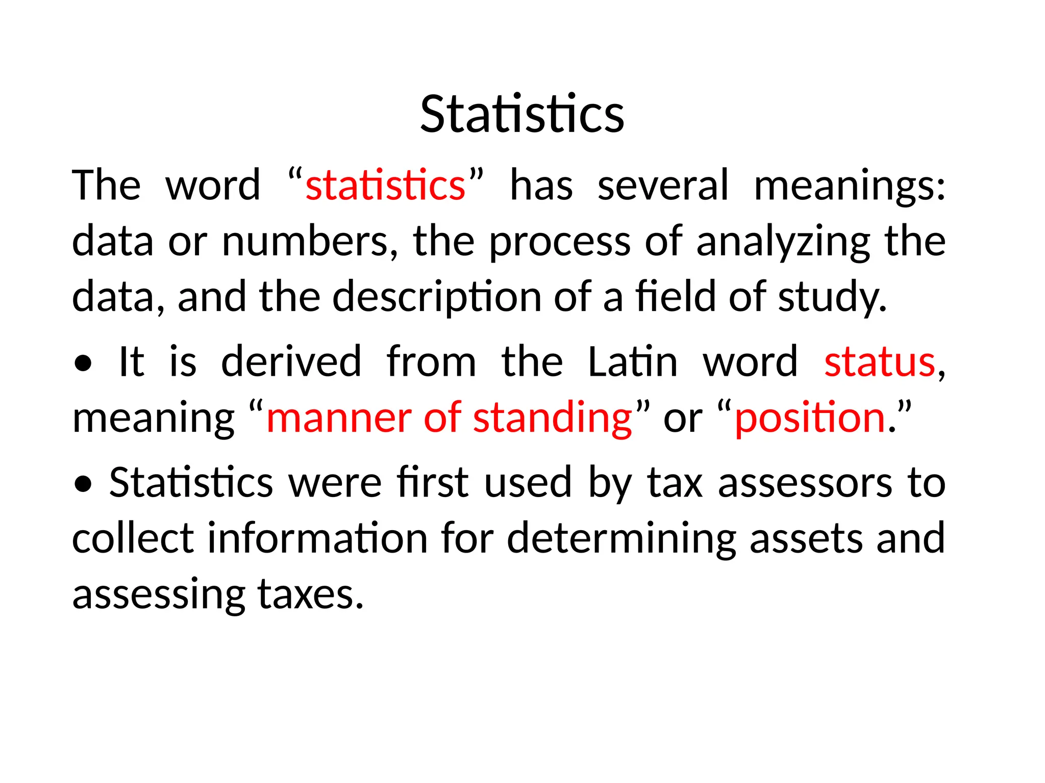
3. Statistics
The word “statistics” has several meanings:
data or numbers, the process of analyzing the
data, and the description of a field of study.
• It is derived from the Latin word status,
meaning “manner of standing” or “position.”
• Statistics were first used by tax assessors to
collect information for determining assets and
assessing taxes.

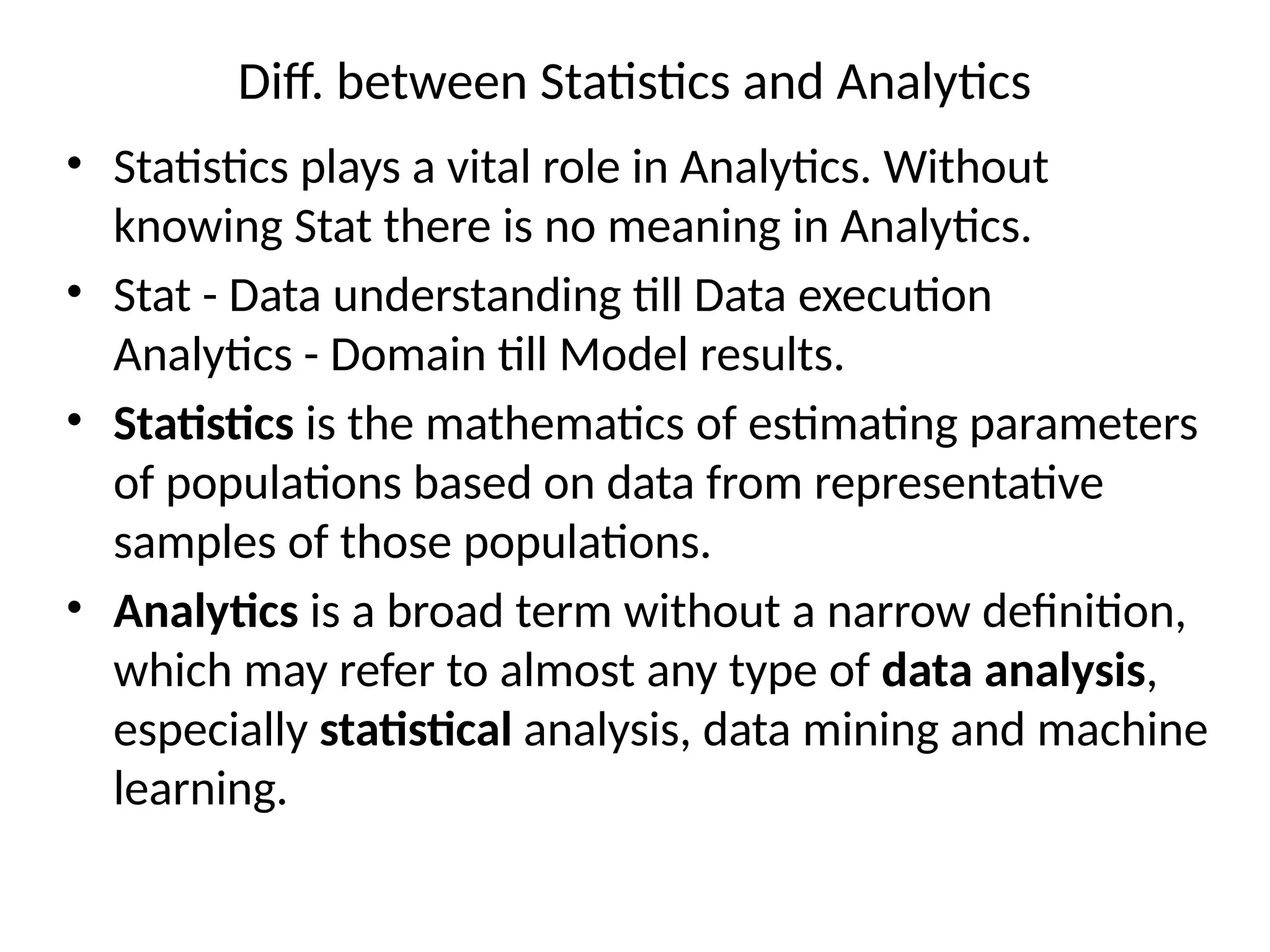
4. Diff. between Statistics and Analytics
• Statistics plays a vital role in Analytics. Without
knowing Stat there is no meaning in Analytics.
• Stat - Data understanding till Data execution
Analytics - Domain till Model results.
• Statistics is the mathematics of estimating parameters
of populations based on data from representative
samples of those populations.
• Analytics is a broad term without a narrow definition,
which may refer to almost any type of data analysis,
especially statistical analysis, data mining and machine
learning.

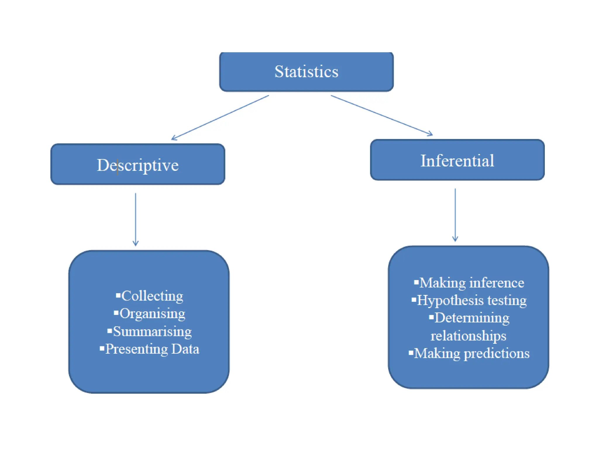
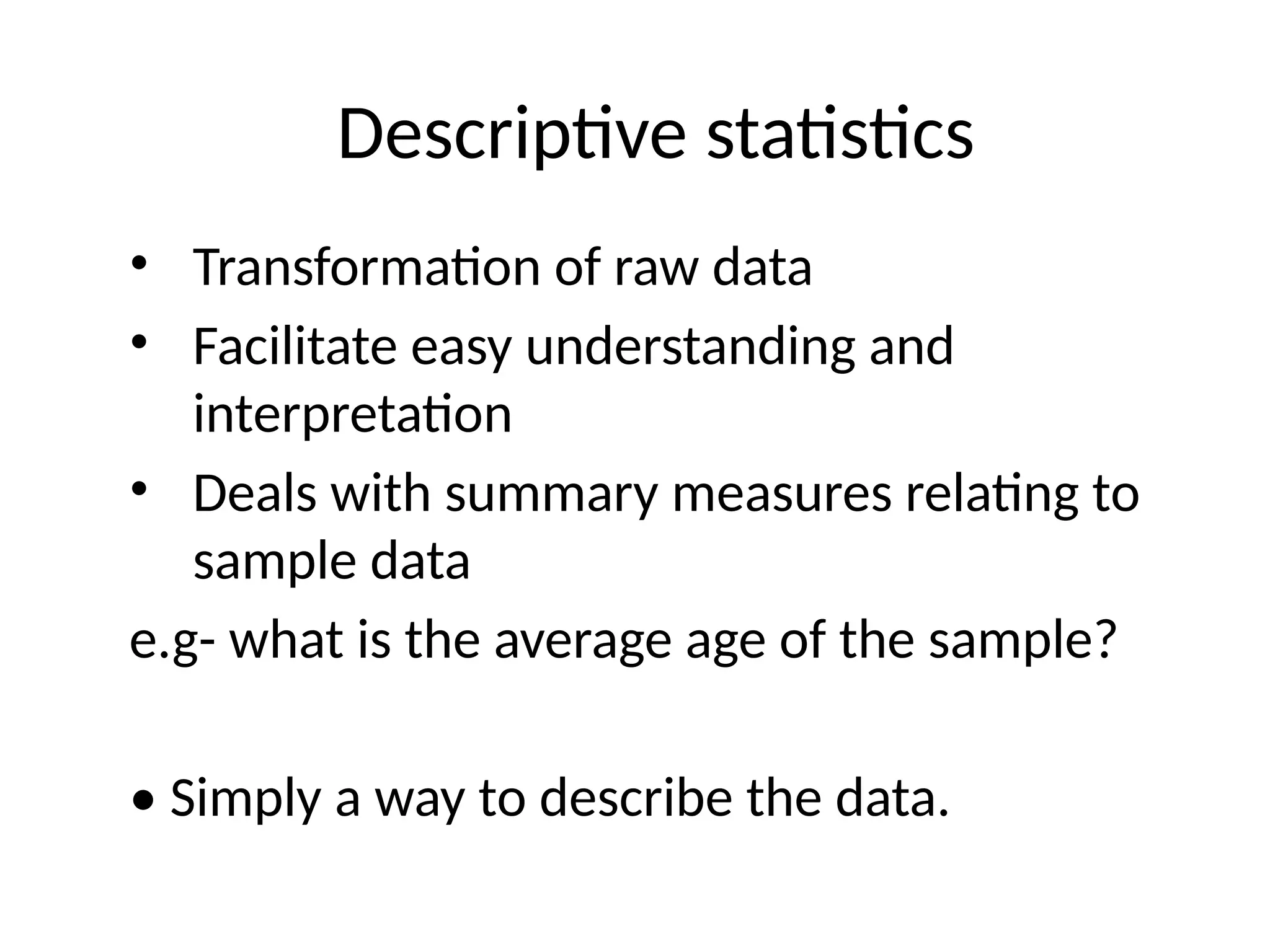
6. Descriptive statistics
• Transformation of raw data
• Facilitate easy understanding and
interpretation
• Deals with summary measures relating to
sample data
e.g- what is the average age of the sample?
• Simply a way to describe the data.

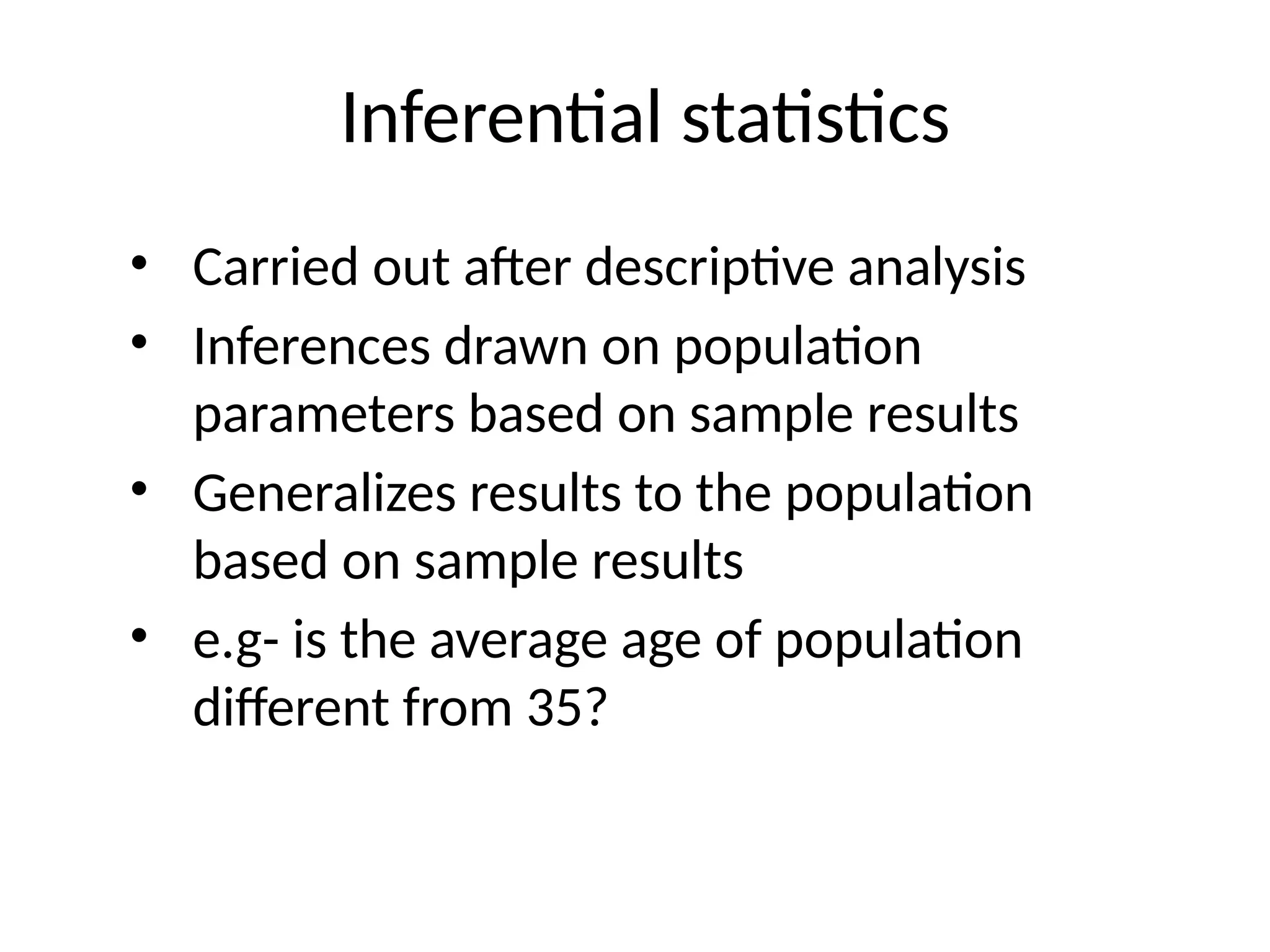
7. Inferential statistics
• Carried out after descriptive analysis
• Inferences drawn on population
parameters based on sample results
• Generalizes results to the population
based on sample results
• e.g- is the average age of population
different from 35?

8. Variable
Variable - Any character, characteristic or quality
that varies is termed a variable.
e.g. - To collect basic clinical and demographic
information on patients with a particular illness. The
variables of interest may include the sex, age and
height of the patients.

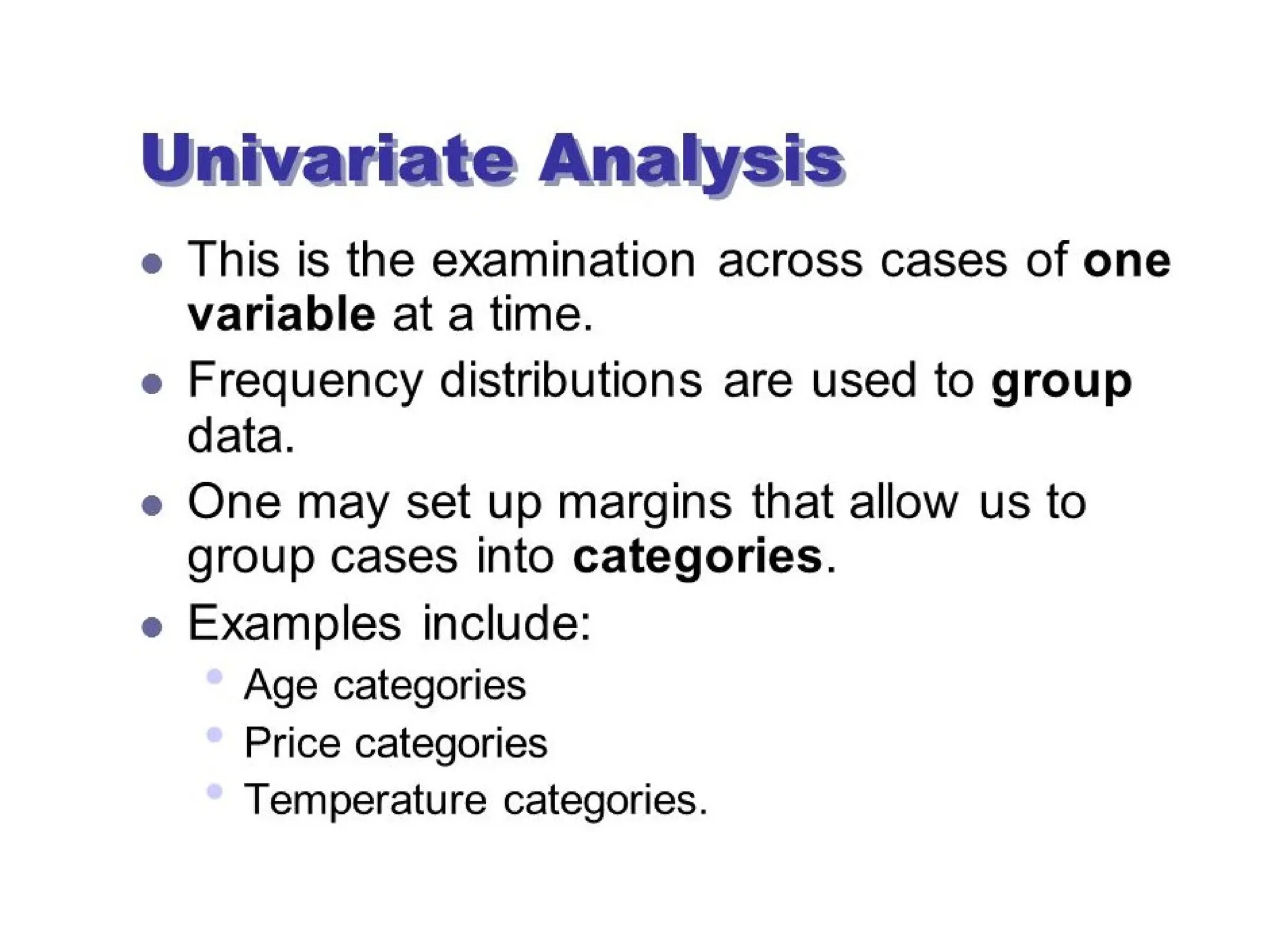
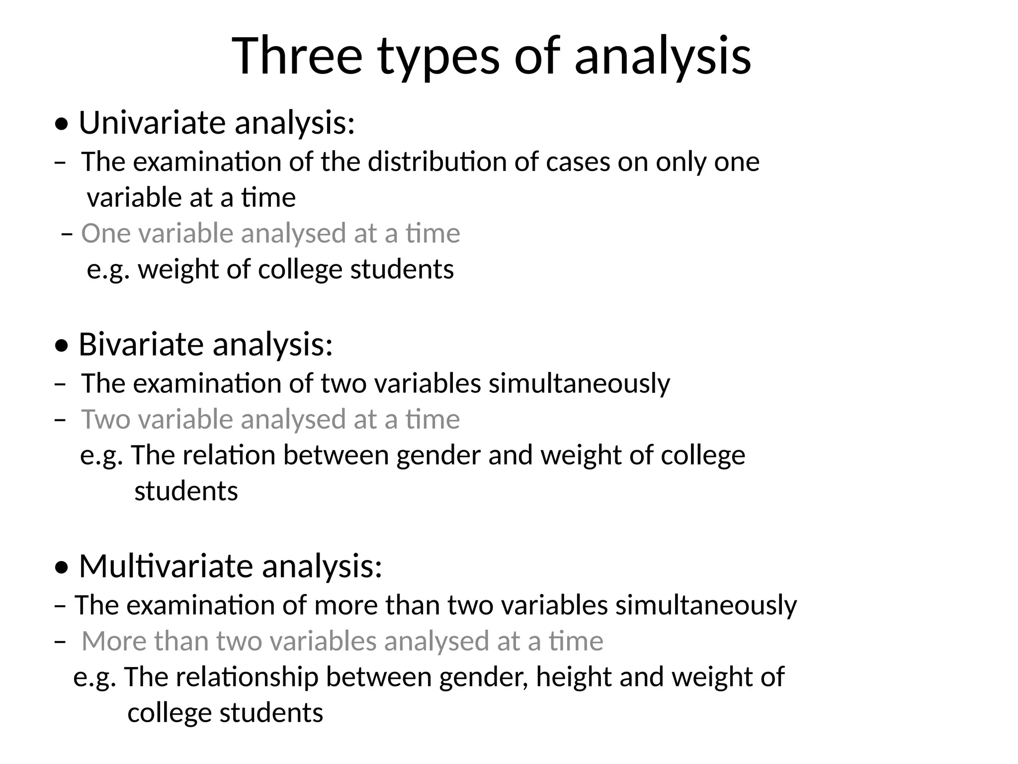
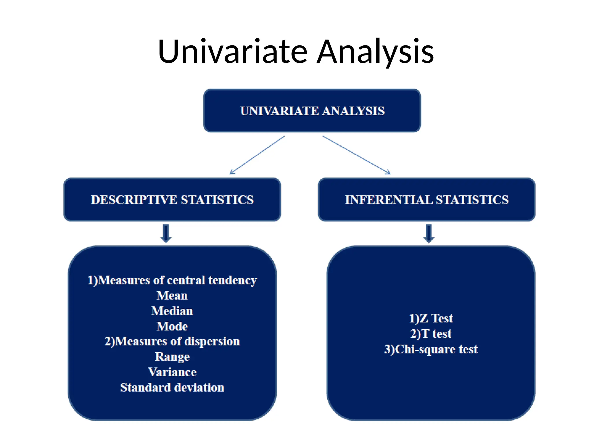
10. Three types of analysis
• Univariate analysis:
– The examination of the distribution of cases on only one
variable at a time
– One variable analysed at a time
e.g. weight of college students
• Bivariate analysis:
– The examination of two variables simultaneously
– Two variable analysed at a time
e.g. The relation between gender and weight of college
students
• Multivariate analysis:
– The examination of more than two variables simultaneously
– More than two variables analysed at a time
e.g. The relationship between gender, height and weight of
college students

11. Purpose of diff. types of analysis
• Univariate analysis
– Purpose: mainly description
• Bivariate analysis
– Purpose: determining the empirical relationship
between the two variables
• Multivariate analysis
– Purpose: determining the empirical relationship
among multiple variables

12. Choosing the Statistical Technique

14. Univariate Analysis

15. Mean, Mode, Median
i] The Mean( Average):
e.g. let's say you have four test scores: 15,
18, 22, and 20.
=(15 + 18 + 22 + 20) / 4
= 75 / 4
= 18.75
If you were to round up to the nearest
whole number, the average would be 19.

16. ii] The Median
• The median is the middle value in a data set.
• To calculate it, place all of your numbers in increasing order.
1] If you have an odd number of integers,
e.g. 3, 9, 15, 17, 44
The middle or median number is =15
2] If you have an even number of data points, then First, find
the two middle integers in your list. Add them together, then
divide by two. The result is the median number.
e.g. 3, 6, 8, 12, 17, 44
The middle or median number is = (8 + 12) / 2
= 20 / 2
= 10

17. iii] Mode
• The mode in a list of numbers refers to the
integers that occur most frequently.
• The mode is about the frequency of
occurrence.
• There can be more than one mode or no
mode at all.
e.g.1) 3, 3, 8, 9, 15, 15, 15, 17, 17, 27, 40, 44, 44
In this case, the mode is= 15.
2) 3, 3, 8, 9, 15, 15, 17, 17, 27, 40, 44, 44
In this case we have four modes: 3, 15, 17, and 44.

18. DATA SCREENING
• Anything that can go wrong will go wrong.
• Data screening (sometimes referred to as
"data screaming") is the process of
ensuring your data is clean and ready to go
before you conduct further statistical
analyses.
• Data must be screened in order to ensure
the data is useable, reliable, and valid for
testing causal theory.

19. PURPOSE OF DATA SCREENING
• Detect and correct data errors
• Detect and treat missing data
• Detect and handle insufficiently sampled
variables
• Conduct transformations and standardizations
• Detect and handle outliers

20. Screening Data Prior to Analysis
• Missing Data
• Outliers
• Normality
• Linearity
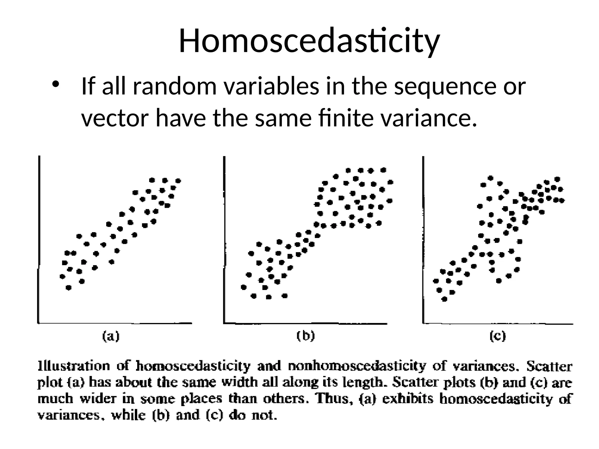
• Homoscedasticity

21. 1] Missing Data
 Missing data may be in following way
• Pattern
• Random
• If the amount of missing data is small don't
really need to worry

22. Why is missing data a problem?
1] Insufficient amount for analysis:
For Small sample The most apparent problem is that there simply won't be
enough data points to run your analyses.
2] Bias sampling:
Missing data might represent bias issues. Some people may not have answered
particular questions in your survey because of some common issue. For example,
if you asked about gender, and females are less likely to report their gender than
males, then you will have male-biased data. Perhaps only 50% of the females
reported their gender, but 95% of the males reported gender. If you use gender
in your causal models, then you will be heavily biased toward males, because you
will not end up using the unreported responses.

23. Why is missing data a problem?
3] Inappropriate measuring procedure
4] Misleading research results
Biased data in, _______ out

24. Treatment for missing data
 Deleting cases or variables
• Descriptive statistics
 Estimating missing data
 Using missing data correlation matrix
 Repeating analyses with and without missing
data
 Choosing among methods for dealing with
missing data
• Pattern or amount

25. 2] Outlier
• Cases with extreme value on variables

26. Outlier
• If you have a really high sample size, then
you may want to remove the outliers.
• If you are working with a smaller dataset,
you may want to be less liberal about
deleting records.
 exert influence on the mean
 inflate variance of the sample

27. Treatment for outlier
 Estimating outlier
• Standardized score (z>2, 2.5, 3)
• Graphical methods (p-p, q-q plot)
• Mahalanobis distance (χ2 test)
 Deletion or transformation
• Critical to analysis or not
• Preservation
1) Transformation
2) Score alternation

28. 3] Normality
• Normality refers to the distribution of the
data for a particular variable.
• We usually assume that the data is normally
distributed, even though it usually is not!
Normality is assessed in many different ways:
 Shape,
 Skewness,
 Kurtosis (flat/peaked).

29. A] Shape
If Shape does not match the normal curve, then you likely have normality
issues.

30. Normal/Symmetrical Distribution
Bell – shaped or unimodel Symmetrical
Distribution
A symmetrical distribution is bell – shaped if
the frequencies are first steadily rise and
then steadily fall.
There is only one mode and the values
of mean, median and mode are equal.
Mean = Median = Mode

31. B] Skewness
• Skewness means that the responses did not fall
into a normal distribution, but were heavily
weighted toward one end of the scale.
• A distribution is said to be 'skewed' when the mean
and the median fall at different points in the
distribution, and the balance (or centre of gravity)
is shifted to one side or the other-to left or right.

32. Positive Skewness
1] If your skewness value is greater than 1
then you are positive (right) skewed.
Positive Skewness indicates a long right tail
Mean ˃ Median ˃ Mode

33. Negative Skewness
2] If it is less than -1 you are negative (left)
skewed.
Mean ˂ Median ˂ Mode
Negative Skewness indicates a long left tail

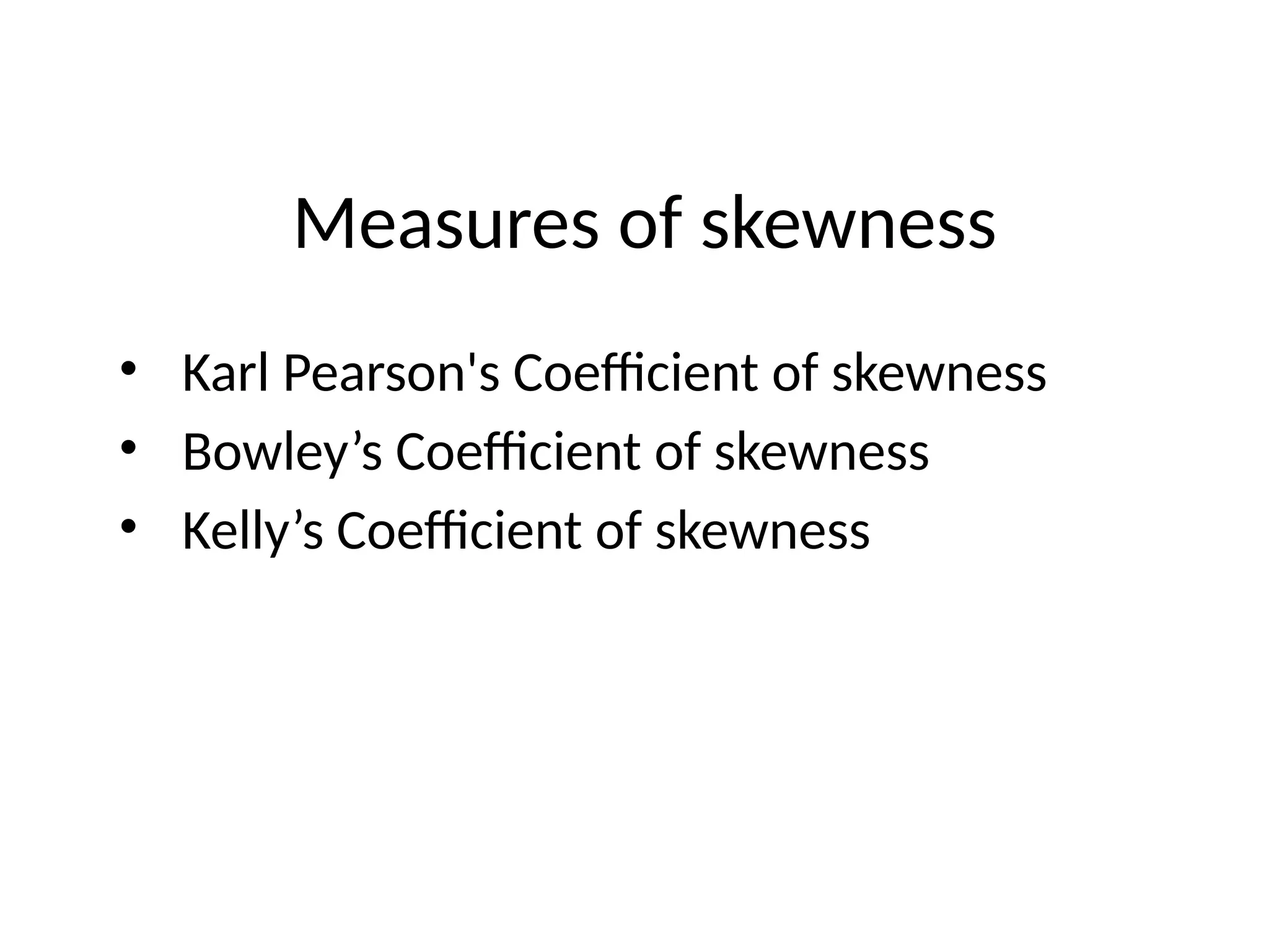
34. Measures of skewness
• Karl Pearson's Coefficient of skewness
• Bowley’s Coefficient of skewness
• Kelly’s Coefficient of skewness

35. 1] Karl Pearson's Coefficient of skewness,
The formula for measuring skewness as given
by Karl Pearson is as follows
Where,
SKP = Karl Pearson's Coefficient of skewness,
σ = standard deviation

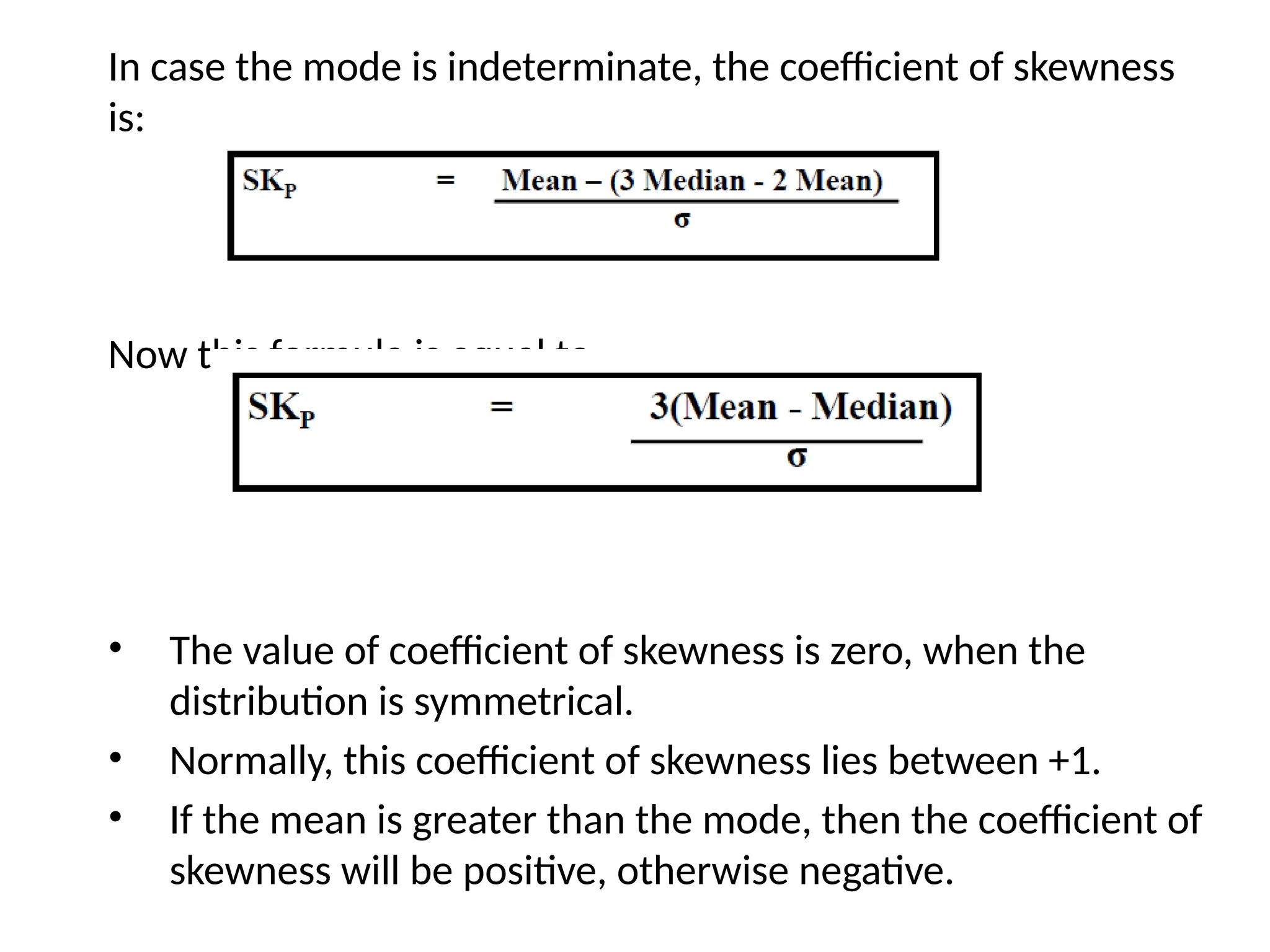
36. In case the mode is indeterminate, the coefficient of skewness
is:
Now this formula is equal to
• The value of coefficient of skewness is zero, when the
distribution is symmetrical.
• Normally, this coefficient of skewness lies between +1.
• If the mean is greater than the mode, then the coefficient of
skewness will be positive, otherwise negative.

37. 2] Bowley’s Coefficient of skewness
Bowley developed a measure of skewness, which
is based on quartile values. The formula for
measuring skewness is:
Where,
SKB = Bowley’s Coefficient of skewness,
Q1 = Quartile first
Q2 = Quartile second
Q3 = Quartile Third

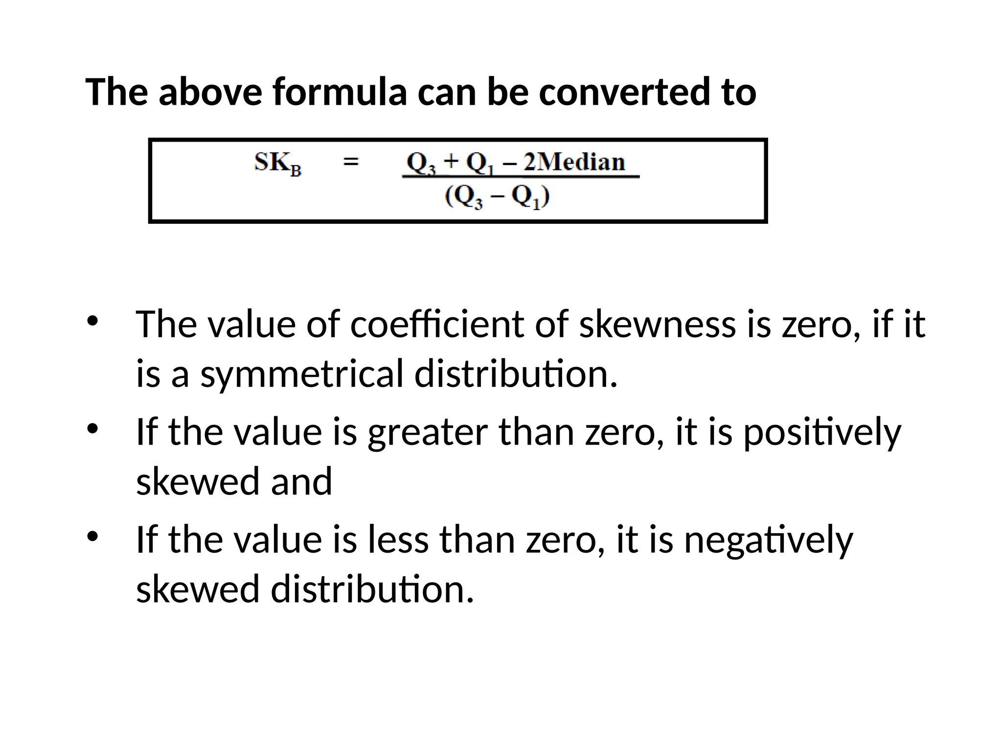
38. The above formula can be converted to
• The value of coefficient of skewness is zero, if it
is a symmetrical distribution.
• If the value is greater than zero, it is positively
skewed and
• If the value is less than zero, it is negatively
skewed distribution.

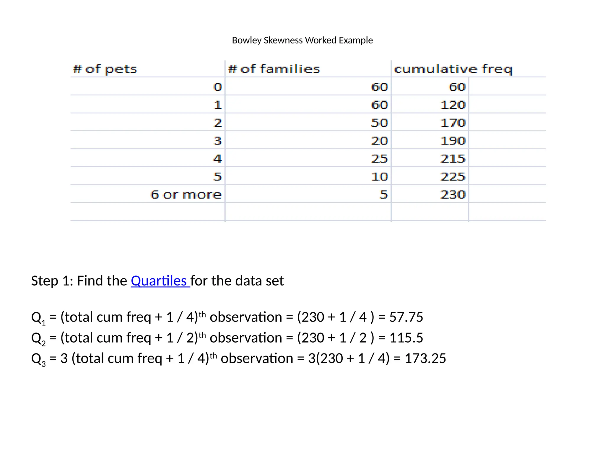
39. Bowley Skewness Worked Example
Step 1: Find the Quartiles for the data set
Q1 = (total cum freq + 1 / 4)th
observation = (230 + 1 / 4 ) = 57.75
Q2 = (total cum freq + 1 / 2)th
observation = (230 + 1 / 2 ) = 115.5
Q3 = 3 (total cum freq + 1 / 4)th
observation = 3(230 + 1 / 4) = 173.25

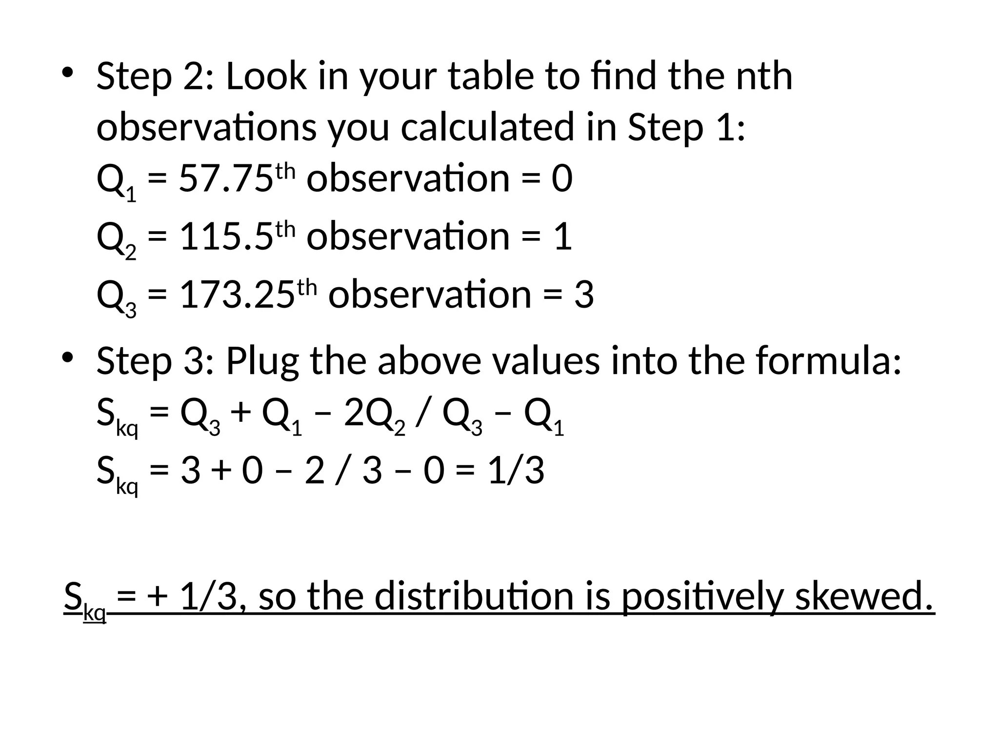
40. • Step 2: Look in your table to find the nth
observations you calculated in Step 1:
Q1 = 57.75th
observation = 0
Q2 = 115.5th
observation = 1
Q3 = 173.25th
observation = 3
• Step 3: Plug the above values into the formula:
Skq = Q3 + Q1 – 2Q2 / Q3 – Q1
Skq = 3 + 0 – 2 / 3 – 0 = 1/3
Skq = + 1/3, so the distribution is positively skewed.

41. 3] Kurtosis
• Kurtosis is another measure of the shape of
a frequency curve.
• It is a Greek word, which means meaning
"curved, arching, bulginess. ".
• In a similar way to the concept of skewness,
kurtosis is a descriptor of the shape of a
probability distribution.
• While skewness signifies the extent of
asymmetry, kurtosis measures the degree of
peakedness of a frequency distribution.

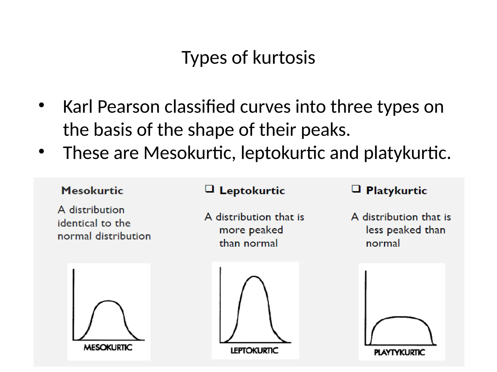
42. Types of kurtosis
• Karl Pearson classified curves into three types on
the basis of the shape of their peaks.
• These are Mesokurtic, leptokurtic and platykurtic.

43. i] Mesokurtic
• Distributions with zero excess
kurtosis are called mesokurtic, or
mesokurtotic.
• The most prominent example of a
mesokurtic distribution is the
normal distribution family,
regardless of the values of its
parameters.
• A few other well-known
distributions can be mesokurtic,
depending on parameter values: for
example, the binomial distribution

44. ii] Leptokurtic
• A distribution with positive excess
kurtosis is called leptokurtic, or
leptokurtotic. "Lepto-" means
"slender".[
In terms of shape, a
leptokurtic distribution has fatter tails.
Examples of leptokurtic distributions
include the
• Student's t- distribution,
• Rayleigh distribution,
• Laplace distribution,
• exponential distribution,
• Poisson distribution and
• logistic distribution.

45. iii]Platykurtic.
• A distribution with negative
excess kurtosis is
called platykurtic, or
platykurtotic. "Platy-" means
"broad".[11]
In terms of shape, a
platykurtic distribution
has thinner tails. Examples of
platykurtic distributions include
the continuous and
discrete uniform distributions,
and the raised cosine distribution.
The most platykurtic distribution
of all is the Bernoulli distribution

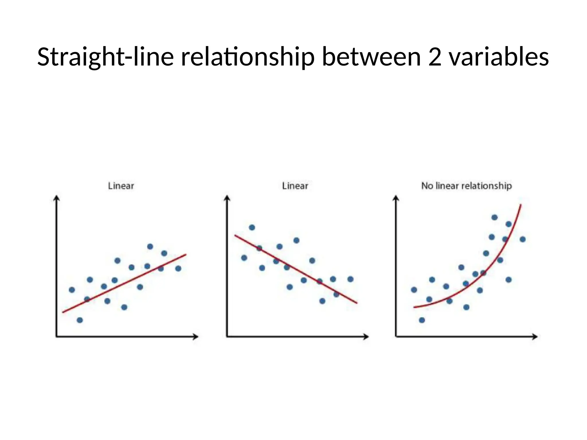
46. 4] Linearity
• linearity is that there is a straight-line relationship
between two variables.
• Linearity between two variables is assessed roughly
by inspection of bivariate scatterplots.
• If both variables are normally distributed and
linearly related, the scatterplot is oval-shaped.
• If one of the variables is non-normal, then the
scatterplot between this variable and the other is
not oval.

47. Straight-line relationship between 2 variables

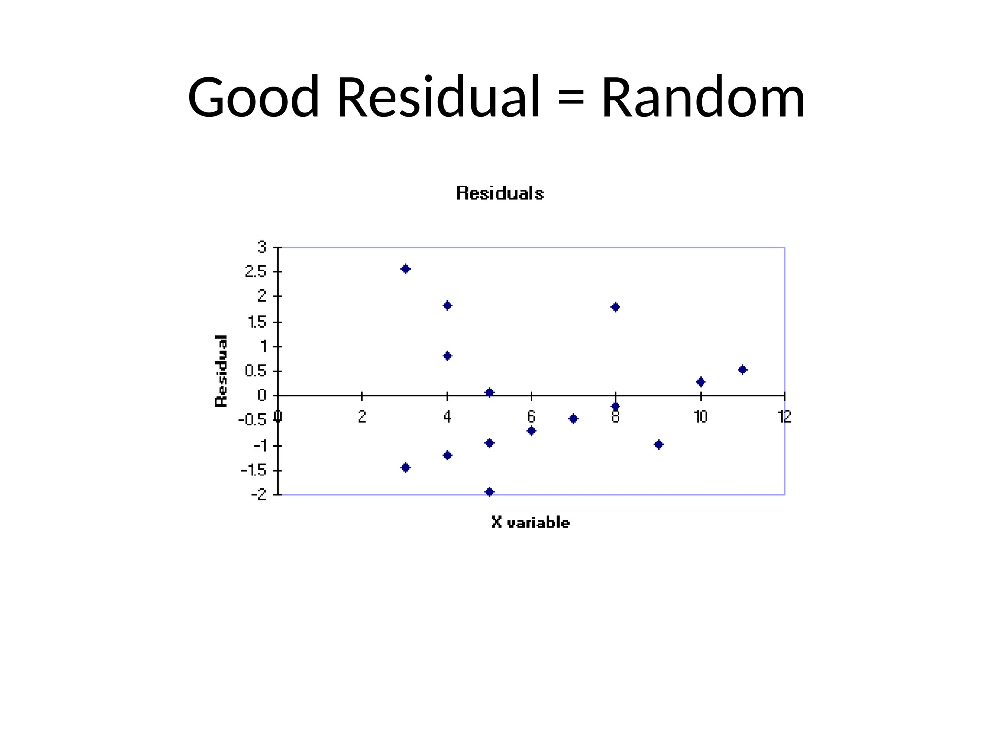
48. Is Linear Model Appropriate?
How do we answer this question?
1. Check SCATTERPLOT and r value for
strong linearity
2. Look at RESIDUAL PLOT—it should
be random

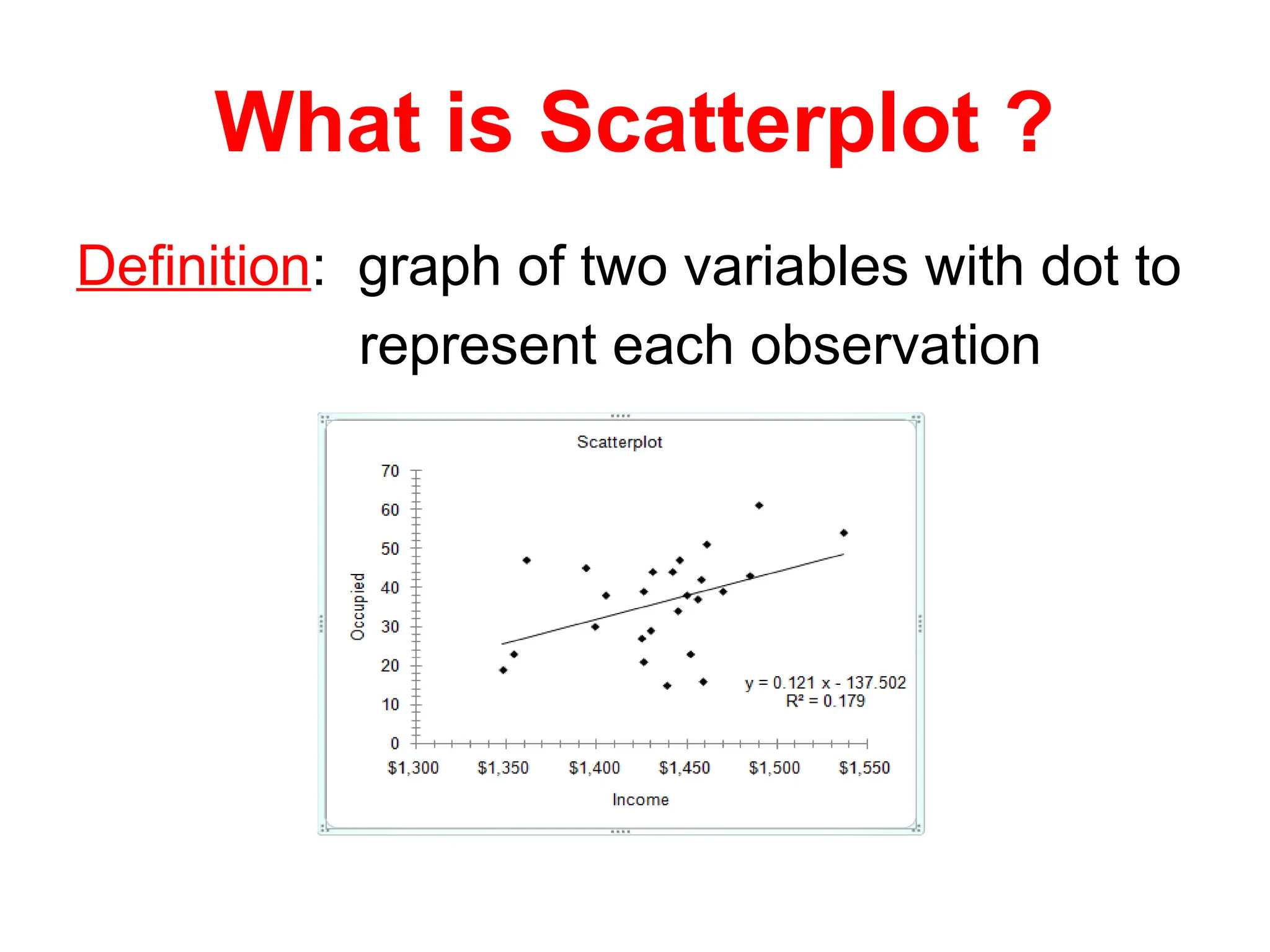
49. What is Scatterplot ?
Definition: graph of two variables with dot to
represent each observation

50. Correlation
Definition: Measures the strength of the
linear relationship between variables
• r is the symbol for correlation
• r takes on values between -1 and 1
• 0 means no linear relationship
• -1 and 1 mean perfect linear relationship

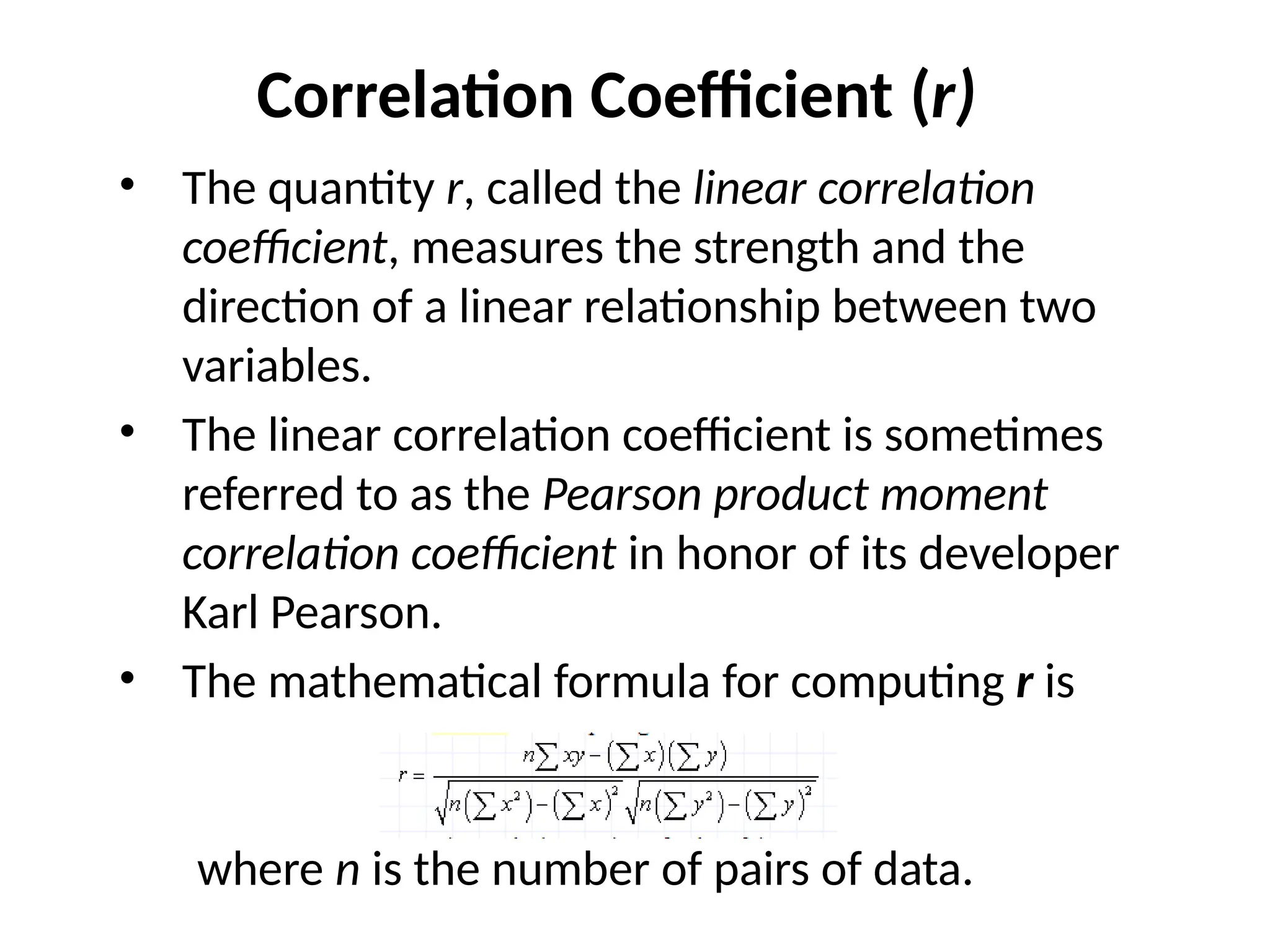
51. Correlation Coefficient (r)
• The quantity r, called the linear correlation
coefficient, measures the strength and the
direction of a linear relationship between two
variables.
• The linear correlation coefficient is sometimes
referred to as the Pearson product moment
correlation coefficient in honor of its developer
Karl Pearson.
• The mathematical formula for computing r is
where n is the number of pairs of data.

52. Positive Correlation
• The value of r is such that -1 < r < +1. The +
and – signs are used for positive linear
correlations and negative linear correlations,
respectively.
• Positive correlation: If x and y have a strong
positive linear correlation, r is close to +1.
An r value of exactly +1 indicates a perfect
positive fit.
• Positive values indicate a relationship
between x and y variables such that as values
for x increases, values for y also increase.

53. Negative Correlation
• Negative correlation: If x and y have a
strong negative linear correlation, r is close
to -1.
• An r value of exactly -1 indicates a perfect
negative fit.
• Negative values indicate a relationship
between x and y such that as values
for x increase, values for y decrease.

54. No correlation
No correlation: If there is no linear correlation
or a weak linear correlation, r is close to 0.
A value near zero means that there is a random,
nonlinear relationship between the two
variables
Note that r is a dimensionless quantity; that is,
it does not depend on the units employed.

55. A perfect correlation of ± 1 occurs only when the data
points all lie exactly on a straight line.
If r = +1, the slope of this line is positive.
If r = -1, the slope of this line is negative.
A correlation greater than 0.8 is generally described
as strong, whereas a correlation less than 0.5 is
generally described as weak.
These values can vary based upon the "type" of data
being examined.
Correlation Coefficient summary

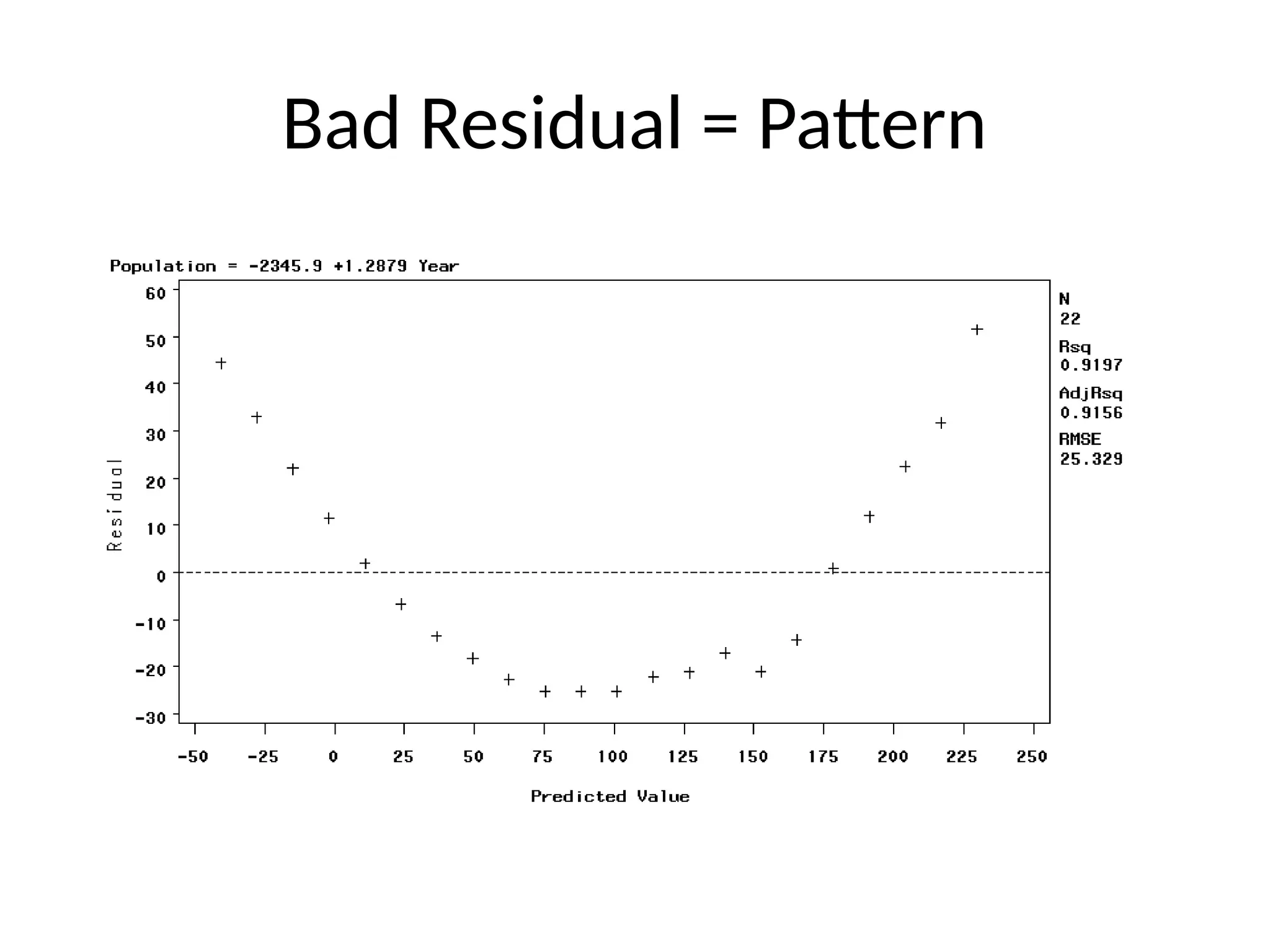
56. RESIDUAL PLOT
A graph of the residual values compared to the x
values.
We do not want to see a pattern of residuals
increasing or decreasing or fitting any
noticeable curve.

57. Good Residual = Random

58. Bad Residual = Pattern

59. Homoscedasticity
• If all random variables in the sequence or
vector have the same finite variance.