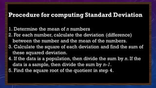
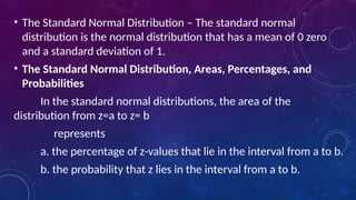
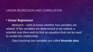
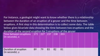
MEASURES OF CENTRAL TENDENCY: EACH MEASURE PROVIDES
A SINGLE VALUE WHICH SUMMARIZES THE SET OF DATA
1. Arithmetic mean or mean – the mean of n
numbers is the sum of the numbers divided by n.
Six friends in a biology class of 20 students
received
test grades of 92, 84, 65, 76, 88, and 90
find the mean of these test scores.
2. Median – the median of a ranked list of n numbers is:
• the middle number if n is odd,
• the mean of the two middle numbers if n is even.
find the median of 4, 8, 1, 14, 9, 21, 12
so, the ranked is 1, 4, 8, 9, 12, 14, 21 and the median is ______?
find the median of 46, 23, 92, 89, 77, 108
3. mode - the mode of a list of numbers is the number occurs most
frequently.
find the mode of
a. 18, 15, 21, 16, 15, 14, 15, 21
b. 2, 5, 8, 9, 11, 4, 7, 23
c. 12, 24, 12, 71, 48, 93, 71
Weighted mean – the value called the weighted mean is often used when some data
values are more important than the others.
the table shows Drillon’s fall semester course grades. use the weighted mean formula to
find his gpa for the fall semester.
Course Course
Grade
Course
Unit
English B=3 4 12
History A=4 3 12
Chemistry D=1 3 3
Algebra C=2 4 8
TRY THIS
SAMPLE PROBLEM
A student has the quiz
scores: 2, 4, 7, 12, 15.
find the standard
deviation for this
population of quiz
scores.
MEASURES OF RELATIVE POSITION
1. Z-Score – The z-score for a given data value x is the number of standard deviations that x
is above or below the mean of the data. The following formulas show how to calculate the
z-score for the value x in a population and in a sample.
Raul has taken two tests in his chemistry class. He scored 72 on the first test, for which the
mean of all scores was 65 and the standard deviation was 8. He received a 60 on a second
test, for which the mean of all scores was 45 and the standard deviation was 12. In
comparison to the other students, did Raul do better on the first test or the second test?
Raul scored 0.875 standard deviation above the mean on the first test and 1.25 standard
deviation above the mean on the second test. The z-scores indicate that, in comparison to
his classmates, Raul scored better on the second test than he did on the first test.
NORMAL CURVE
68.26%
95.44%
2. pth Percentile- A value x is called the pth percentile of a data set
provides of the data values are less than x.
In a recent year, the median annual salary for a physical therapist was $74,480. If the 90th
percentile for the annual salary of a PT was $105,900, find the percent of physical
therapists whose annual salary was
a. More than $74,480. ans. 50% of the PT earned more than $74,480 per year
b. Less than $105,900. ans. 90%of all PT made less than $105,900.
c. Between $74,480 and $105,900. ans. 90%-50% = 40% of the PT earned $74,480 and
105,900.
Percentile for a Given Data Value
Given a set of data and a data value x,
On a reading examination given to 900 students, Elaine’s
score of 602 was higher than the scores of 576 of the
students of the students who took the examination. What is
the percentile for Elaine’s score?
Ans. Elaine’s score of 602 places her at the 64th
percentile.
3. Quartiles – The three that partition a ranked data set into four (approximately)
equal groups are called the quartiles of the data. For instance, for the data set below,
the values
are the quartiles of the data.
2, 5, 5, 8, 11, 12, 19, 22, 23, 29, 31, 45, 83, 91, 104, 159, 181, 312,
354,
The Median Procedure for Finding Quartiles
1. Rank the data.
2. Find the median of the data. This is the second quartile, Q2.
3. The firs quartile, Q1, is the median of the data values less than Q2. The third
quartile,
Q3, is the median of the data values greater than Q2.
The following table lists the calories per 100
milliliters of 25 popular sodas. Find the quartiles
for the data.
43 37 42 40 53 62 36 32 50 49
26 53 73 48 45 39 45 48 40 56
41 36 58 42 39
•Box-and-Whisker Plots – A box-and-whisker
plot is often used to provide a visual
summary of a set of data. A box-and-
whisker plot shows the median, the first
and third quartiles, and the minimum and
maximum values of a data set.
Construction of a Box-and-Whisker Plot
1. Draw a horizontal scale that extends from the minimum data value
to the maximum data value.
2. Above the scale, draw a rectangle (box) with its left side at Q1 and its
right side at Q3.
3. Draw a vertical line segment across the rectangle at the median, Q2.
4. Draw a horizontal line segment, called a whisker, that extends from
Q1 to the minimum and another whisker that extends from Q3 to the
maximum.
• Stem-and-Leaf Diagrams – The relative position of each data value in a small set of data can be graphically displayed by
using a stem-and leaf diagram. For instance, consider the following history test score.
65, 72, 96, 86, 43, 61, 75, 86, 98, 74, 84, 78, 85, 75, 86, 73
Legend: 8/6 represents 86
Steps in Construction of a Stem-and-Leaf Diagram
1. Determine the stems and list them in a column from smallest to largest or largest to smallest.
2. List the remaining digit of each stem as a leaf to the right of the stem.
3. Include a legend that explains the meaning of the stems and the leaves. Include the title of the diagram.
Stems Leaves
4 3
5
6 1 5
7 2 3 4 5 5 8
8 4 5 6 6 6
9 6 8
NORMAL DISTRIBUTIONS
Frequency Distributions and Histograms – Large sets of data are often displayed using grouped frequency distribution or
a histogram. For instance, consider the following distribution.
Download Time (in seconds) Number of subscribers Percent of subscribers
0-5 6 0.6
5-10 17 1.7
10-15 43 4.3
15-20 92 9.2
20-25 151 15.1
25-30 192 19.2
30-35 190 19.0
35-40 149 14.9
40-45 90 9.0
45-50 45 4.5
50-55 15 1.5
55-60 10 1.0
• Use the relative frequency distribution to determine the
a. percent of subscribers who required at least 25s to download the file.
b. probability that a subscriber chosen at random will require at least 5s but
less than 20s to download the file.
Solution:
a. The percent of data in all the classes with a lower boundary of 25s or more is the sum
of the percent. Thus the percent of subscribers who required at least 25s to download
the file is 69.1%.
b. The percent of data in all the classes with a boundary of 5s and an upper boundary of
20s is the sum of the percent. Thus the percent of subscribers who required at least 5s
but less than 20s to download the file is 15.2%. The probability that a subscriber
chosen at random will require at least 5s but less than 20s to download the file is 0.152.
• Properties of a Normal Distribution
Every normal distribution has the following properties:
1. The graph is symmetric about a vertical line through the mean of
the distribution.
2. The mean, median, and mode are equal.
3. The y-value of each point on the curve is the percent (expressed
as a decimal) of the data at the corresponding x-value.
4. Areas under the curve that are symmetric about the mean are
equal.
5. The total area under the curve is 1.
Empirical Rule for a Normal Distribution
In a normal distribution, approximately
1. 68% of the data lie within 1 standard deviation of the mean.
2. 95% of the data lie within 2 standard deviation of the mean
3. 99.7% of the data lie within 3 standard deviation of the
mean
A survey of 1000 U.S. gas stations that the price charged for a gallon of
regular gas could be closely approximated by a normal distribution with a
mean of $3.10 and a standard deviation
of $0.18. How many of the station charge
a. between $2.74 and $3.46 for a gallon of regular gas?
b. less than $3.28 for a gallon of regular gas?
c. more than $3.46 for a gallon of regular gas?
Solution
a. 950
b. 840
c. 25
• The Standard Normal Distribution – The standard normal
distribution is the normal distribution that has a mean of 0 zero
and a standard deviation of 1.
• The Standard Normal Distribution, Areas, Percentages, and
Probabilities
In the standard normal distributions, the area of the
distribution from z=a to z= b
represents
a. the percentage of z-values that lie in the interval from a to b.
b. the probability that z lies in the interval from a to b.
A soda machine dispenses soda into 12-ounce cups. Tests show
that the actual amount of soda
dispensed is normally distributed, with a mean of 11.5 ounce and
a standard deviation of 0.2 oz.
1. What percent of cups will receive less than 11.25 oz of
soda?
2. What percent of cups will receive between 11.2 oz and
11.55 oz of soda?
3. If a cup is filled at random, what is the probability that
the machine will overflow the cup?
LINEAR REGRESSION AND CORRELATION
• Linear Regression
Research – wish to know whether two variables are
related. If the variables are determined to be related, a
scientist may then wish to find an equation that can be used
to model the relationship.
Data involving two variables are called bivariate data.
For instance, a geologist might want to know whether there is a relationship
between the duration of an eruption of a geyser and the time between
eruptions. A first step in this determination is to collect some data. The table
below gives bivariate data showing the time between two eruptions and the
duration of the second eruption for 5 eruptions of the geyser
Time between eruptions
(in seconds), x
272 227 237 238 203
Duration of eruption
(in seconds), y
89 79 83 82 81
LINEAR REGRESSION AND CORRELATION
The Least-Square Regression Line
The least-squares regression line for a set
of bivariate data is the line that minimizes the
sum of the squares of the vertical deviations
from each data point to the line.
LINEAR REGRESSION AND CORRELATION
The Least-Square Regression Line
Formula
 
 
 
x
a
y
b
x
x
n
y
x
xy
n
a
b
ax
y












and
where
,
ˆ
2
2
Time between
eruptions (in
seconds), x
Duration of
eruption
(in seconds),
y XY X2
272 89 24,208 73,984 87.48
227 79 17,933 51,529 81.73
237 83 19,671 56,169
83.00
238 82 19,516 56,644 83.13
203 81 16,443 41,209 78.66
1,177 414 97,771 279,535
• Interpolation – The process of using an
equation to determine a
point between given data
points.
• Extrapolation – The process of using an
equation to determine a
point to the right or left of
a given data points.
• Linear Correlation Coefficient – To determine the strength of a
linear relationship between two variables
If the linear correlation coefficient r is positive, the relationship
between the variables has a positive correlation.
In this case, if one variable increases, the other variable also tends to
increase.
If r is negative, the relationship between the variables has a negative
correlation. In this case, if one variable increases, the other variable
tends to decrease.
The linear correlation coefficient indicates the strength of a linear
relationship between two variables; however, it does not indicate the
presence of a cause-and-effect relationship. For instance, the data in the
table below show the hours per week that a student spent playing pool
and the student’s weekly algebra test scores for those same weeks.
Use the linear correlation coefficient formula to verify
r = 0.98
Hours per week spent playing pool 4 5 7 8 10
Weekly algebra test score 52 60 72 79 83
X Y x2 y2 xy
4 52 16 2704 208
5 60 25 3600 300
7 72 49 5184 504
8 79 64 6241 632
10 83 100 6889 830
34 346 254 24618 2474
The linear correlation coefficient for the ordered pairs in the
table is r = 0.98. Thus there is a strong or very high positive linear
relationship between the student’s algebra test score and the
time the student spent playing pool. This does not mean that the
higher algebra test scores were caused by the increased time
spent playing pool. The fact that the student’s test scores
increased with the increase in the time spent playing pool could
be due to many factors, or it could just be a coincidence.
Guilford’s suggested interpretation for values
of r.
r value Interpretation
Less than .20 Slight; almost negligible relationship
.20 - .40 Low correlation; definite but small relationship
.40 - .70 Moderate correlation; substantial relationship
.70 - .90 High correlation; marked relationship
.90 - 1.00 Very high correlation; very dependable
relationship
Descriptive Stat numerical_-112700052.pptx

Descriptive Stat numerical_-112700052.pptx

  • 1.
    MEASURES OF CENTRALTENDENCY: EACH MEASURE PROVIDES A SINGLE VALUE WHICH SUMMARIZES THE SET OF DATA 1. Arithmetic mean or mean – the mean of n numbers is the sum of the numbers divided by n. Six friends in a biology class of 20 students received test grades of 92, 84, 65, 76, 88, and 90 find the mean of these test scores.
  • 2.
    2. Median –the median of a ranked list of n numbers is: • the middle number if n is odd, • the mean of the two middle numbers if n is even. find the median of 4, 8, 1, 14, 9, 21, 12 so, the ranked is 1, 4, 8, 9, 12, 14, 21 and the median is ______? find the median of 46, 23, 92, 89, 77, 108 3. mode - the mode of a list of numbers is the number occurs most frequently. find the mode of a. 18, 15, 21, 16, 15, 14, 15, 21 b. 2, 5, 8, 9, 11, 4, 7, 23 c. 12, 24, 12, 71, 48, 93, 71
  • 3.
    Weighted mean –the value called the weighted mean is often used when some data values are more important than the others. the table shows Drillon’s fall semester course grades. use the weighted mean formula to find his gpa for the fall semester. Course Course Grade Course Unit English B=3 4 12 History A=4 3 12 Chemistry D=1 3 3 Algebra C=2 4 8
  • 4.
  • 7.
    SAMPLE PROBLEM A studenthas the quiz scores: 2, 4, 7, 12, 15. find the standard deviation for this population of quiz scores.
  • 16.
    MEASURES OF RELATIVEPOSITION 1. Z-Score – The z-score for a given data value x is the number of standard deviations that x is above or below the mean of the data. The following formulas show how to calculate the z-score for the value x in a population and in a sample. Raul has taken two tests in his chemistry class. He scored 72 on the first test, for which the mean of all scores was 65 and the standard deviation was 8. He received a 60 on a second test, for which the mean of all scores was 45 and the standard deviation was 12. In comparison to the other students, did Raul do better on the first test or the second test? Raul scored 0.875 standard deviation above the mean on the first test and 1.25 standard deviation above the mean on the second test. The z-scores indicate that, in comparison to his classmates, Raul scored better on the second test than he did on the first test.
  • 17.
  • 18.
    2. pth Percentile-A value x is called the pth percentile of a data set provides of the data values are less than x. In a recent year, the median annual salary for a physical therapist was $74,480. If the 90th percentile for the annual salary of a PT was $105,900, find the percent of physical therapists whose annual salary was a. More than $74,480. ans. 50% of the PT earned more than $74,480 per year b. Less than $105,900. ans. 90%of all PT made less than $105,900. c. Between $74,480 and $105,900. ans. 90%-50% = 40% of the PT earned $74,480 and 105,900. Percentile for a Given Data Value Given a set of data and a data value x,
  • 19.
    On a readingexamination given to 900 students, Elaine’s score of 602 was higher than the scores of 576 of the students of the students who took the examination. What is the percentile for Elaine’s score? Ans. Elaine’s score of 602 places her at the 64th percentile.
  • 20.
    3. Quartiles –The three that partition a ranked data set into four (approximately) equal groups are called the quartiles of the data. For instance, for the data set below, the values are the quartiles of the data. 2, 5, 5, 8, 11, 12, 19, 22, 23, 29, 31, 45, 83, 91, 104, 159, 181, 312, 354, The Median Procedure for Finding Quartiles 1. Rank the data. 2. Find the median of the data. This is the second quartile, Q2. 3. The firs quartile, Q1, is the median of the data values less than Q2. The third quartile, Q3, is the median of the data values greater than Q2.
  • 21.
    The following tablelists the calories per 100 milliliters of 25 popular sodas. Find the quartiles for the data. 43 37 42 40 53 62 36 32 50 49 26 53 73 48 45 39 45 48 40 56 41 36 58 42 39
  • 22.
    •Box-and-Whisker Plots –A box-and-whisker plot is often used to provide a visual summary of a set of data. A box-and- whisker plot shows the median, the first and third quartiles, and the minimum and maximum values of a data set.
  • 23.
    Construction of aBox-and-Whisker Plot 1. Draw a horizontal scale that extends from the minimum data value to the maximum data value. 2. Above the scale, draw a rectangle (box) with its left side at Q1 and its right side at Q3. 3. Draw a vertical line segment across the rectangle at the median, Q2. 4. Draw a horizontal line segment, called a whisker, that extends from Q1 to the minimum and another whisker that extends from Q3 to the maximum.
  • 24.
    • Stem-and-Leaf Diagrams– The relative position of each data value in a small set of data can be graphically displayed by using a stem-and leaf diagram. For instance, consider the following history test score. 65, 72, 96, 86, 43, 61, 75, 86, 98, 74, 84, 78, 85, 75, 86, 73 Legend: 8/6 represents 86 Steps in Construction of a Stem-and-Leaf Diagram 1. Determine the stems and list them in a column from smallest to largest or largest to smallest. 2. List the remaining digit of each stem as a leaf to the right of the stem. 3. Include a legend that explains the meaning of the stems and the leaves. Include the title of the diagram. Stems Leaves 4 3 5 6 1 5 7 2 3 4 5 5 8 8 4 5 6 6 6 9 6 8
  • 25.
    NORMAL DISTRIBUTIONS Frequency Distributionsand Histograms – Large sets of data are often displayed using grouped frequency distribution or a histogram. For instance, consider the following distribution. Download Time (in seconds) Number of subscribers Percent of subscribers 0-5 6 0.6 5-10 17 1.7 10-15 43 4.3 15-20 92 9.2 20-25 151 15.1 25-30 192 19.2 30-35 190 19.0 35-40 149 14.9 40-45 90 9.0 45-50 45 4.5 50-55 15 1.5 55-60 10 1.0
  • 26.
    • Use therelative frequency distribution to determine the a. percent of subscribers who required at least 25s to download the file. b. probability that a subscriber chosen at random will require at least 5s but less than 20s to download the file. Solution: a. The percent of data in all the classes with a lower boundary of 25s or more is the sum of the percent. Thus the percent of subscribers who required at least 25s to download the file is 69.1%. b. The percent of data in all the classes with a boundary of 5s and an upper boundary of 20s is the sum of the percent. Thus the percent of subscribers who required at least 5s but less than 20s to download the file is 15.2%. The probability that a subscriber chosen at random will require at least 5s but less than 20s to download the file is 0.152.
  • 27.
    • Properties ofa Normal Distribution Every normal distribution has the following properties: 1. The graph is symmetric about a vertical line through the mean of the distribution. 2. The mean, median, and mode are equal. 3. The y-value of each point on the curve is the percent (expressed as a decimal) of the data at the corresponding x-value. 4. Areas under the curve that are symmetric about the mean are equal. 5. The total area under the curve is 1.
  • 29.
    Empirical Rule fora Normal Distribution In a normal distribution, approximately 1. 68% of the data lie within 1 standard deviation of the mean. 2. 95% of the data lie within 2 standard deviation of the mean 3. 99.7% of the data lie within 3 standard deviation of the mean
  • 30.
    A survey of1000 U.S. gas stations that the price charged for a gallon of regular gas could be closely approximated by a normal distribution with a mean of $3.10 and a standard deviation of $0.18. How many of the station charge a. between $2.74 and $3.46 for a gallon of regular gas? b. less than $3.28 for a gallon of regular gas? c. more than $3.46 for a gallon of regular gas? Solution a. 950 b. 840 c. 25
  • 31.
    • The StandardNormal Distribution – The standard normal distribution is the normal distribution that has a mean of 0 zero and a standard deviation of 1. • The Standard Normal Distribution, Areas, Percentages, and Probabilities In the standard normal distributions, the area of the distribution from z=a to z= b represents a. the percentage of z-values that lie in the interval from a to b. b. the probability that z lies in the interval from a to b.
  • 32.
    A soda machinedispenses soda into 12-ounce cups. Tests show that the actual amount of soda dispensed is normally distributed, with a mean of 11.5 ounce and a standard deviation of 0.2 oz. 1. What percent of cups will receive less than 11.25 oz of soda? 2. What percent of cups will receive between 11.2 oz and 11.55 oz of soda? 3. If a cup is filled at random, what is the probability that the machine will overflow the cup?
  • 33.
    LINEAR REGRESSION ANDCORRELATION • Linear Regression Research – wish to know whether two variables are related. If the variables are determined to be related, a scientist may then wish to find an equation that can be used to model the relationship. Data involving two variables are called bivariate data.
  • 34.
    For instance, ageologist might want to know whether there is a relationship between the duration of an eruption of a geyser and the time between eruptions. A first step in this determination is to collect some data. The table below gives bivariate data showing the time between two eruptions and the duration of the second eruption for 5 eruptions of the geyser Time between eruptions (in seconds), x 272 227 237 238 203 Duration of eruption (in seconds), y 89 79 83 82 81
  • 35.
    LINEAR REGRESSION ANDCORRELATION The Least-Square Regression Line The least-squares regression line for a set of bivariate data is the line that minimizes the sum of the squares of the vertical deviations from each data point to the line.
  • 36.
    LINEAR REGRESSION ANDCORRELATION The Least-Square Regression Line Formula       x a y b x x n y x xy n a b ax y             and where , ˆ 2 2
  • 37.
    Time between eruptions (in seconds),x Duration of eruption (in seconds), y XY X2 272 89 24,208 73,984 87.48 227 79 17,933 51,529 81.73 237 83 19,671 56,169 83.00 238 82 19,516 56,644 83.13 203 81 16,443 41,209 78.66 1,177 414 97,771 279,535
  • 38.
    • Interpolation –The process of using an equation to determine a point between given data points. • Extrapolation – The process of using an equation to determine a point to the right or left of a given data points.
  • 39.
    • Linear CorrelationCoefficient – To determine the strength of a linear relationship between two variables If the linear correlation coefficient r is positive, the relationship between the variables has a positive correlation. In this case, if one variable increases, the other variable also tends to increase. If r is negative, the relationship between the variables has a negative correlation. In this case, if one variable increases, the other variable tends to decrease.
  • 40.
    The linear correlationcoefficient indicates the strength of a linear relationship between two variables; however, it does not indicate the presence of a cause-and-effect relationship. For instance, the data in the table below show the hours per week that a student spent playing pool and the student’s weekly algebra test scores for those same weeks. Use the linear correlation coefficient formula to verify r = 0.98 Hours per week spent playing pool 4 5 7 8 10 Weekly algebra test score 52 60 72 79 83
  • 41.
    X Y x2y2 xy 4 52 16 2704 208 5 60 25 3600 300 7 72 49 5184 504 8 79 64 6241 632 10 83 100 6889 830 34 346 254 24618 2474
  • 42.
    The linear correlationcoefficient for the ordered pairs in the table is r = 0.98. Thus there is a strong or very high positive linear relationship between the student’s algebra test score and the time the student spent playing pool. This does not mean that the higher algebra test scores were caused by the increased time spent playing pool. The fact that the student’s test scores increased with the increase in the time spent playing pool could be due to many factors, or it could just be a coincidence.
  • 43.
    Guilford’s suggested interpretationfor values of r. r value Interpretation Less than .20 Slight; almost negligible relationship .20 - .40 Low correlation; definite but small relationship .40 - .70 Moderate correlation; substantial relationship .70 - .90 High correlation; marked relationship .90 - 1.00 Very high correlation; very dependable relationship