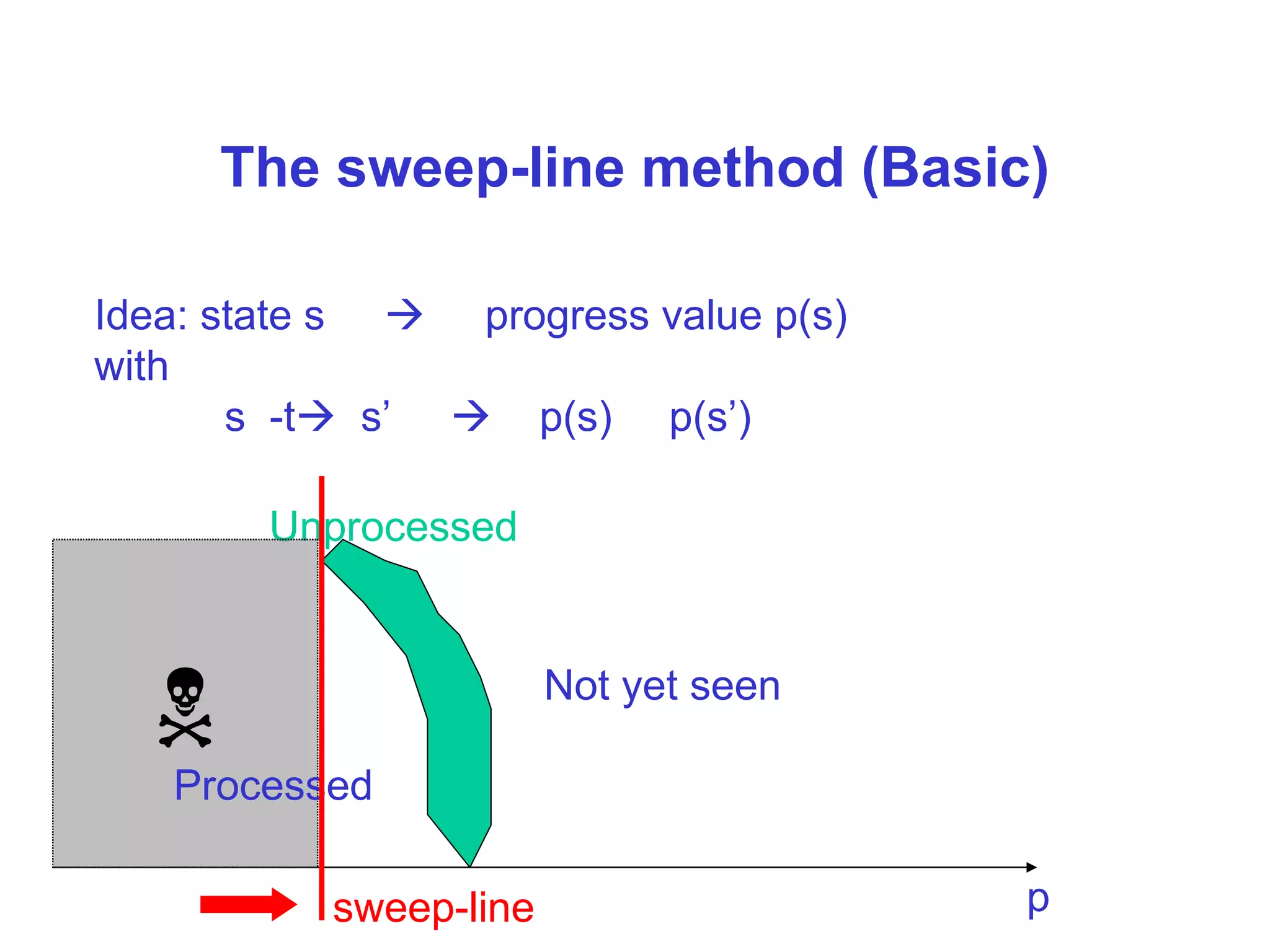
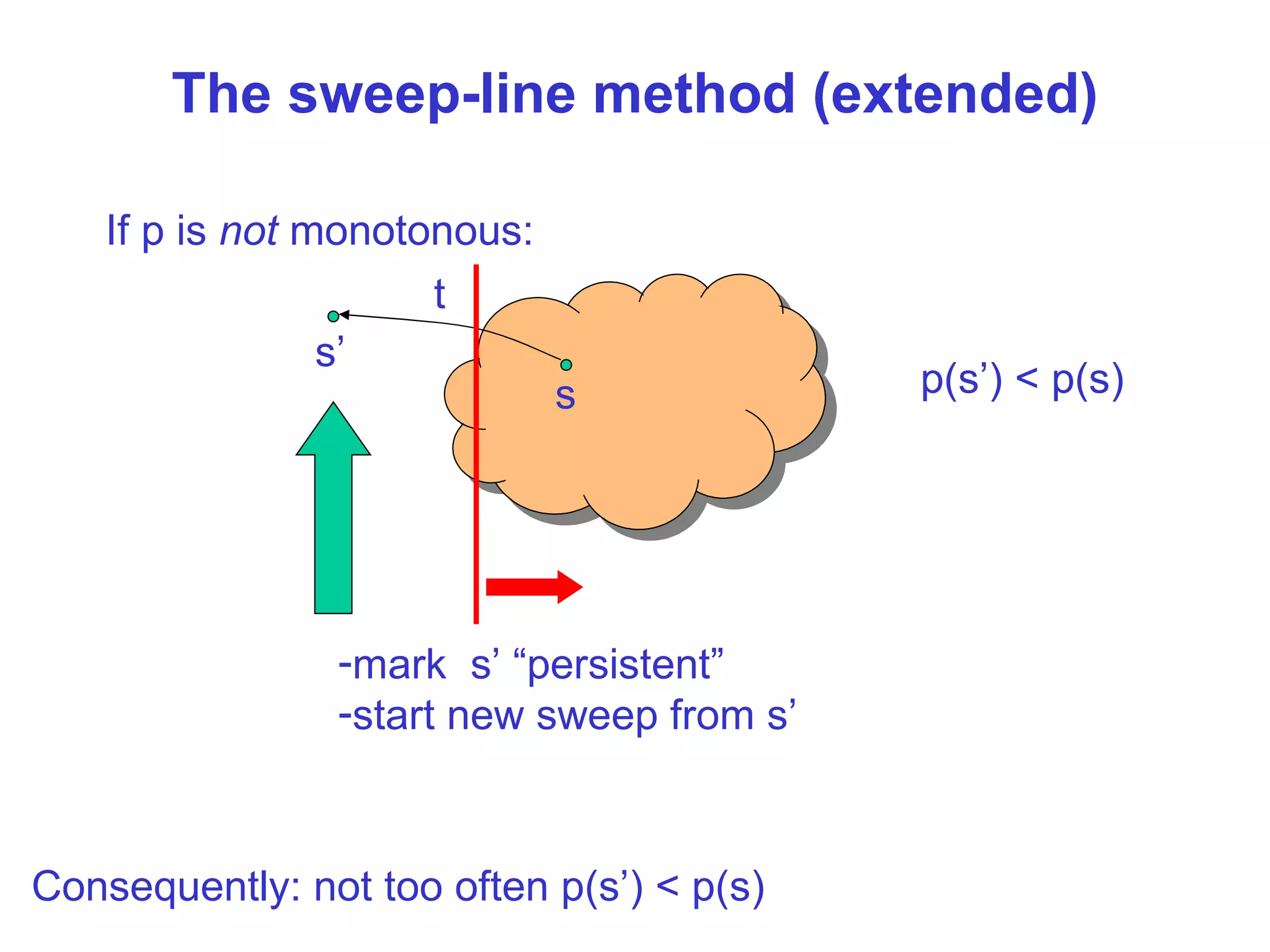
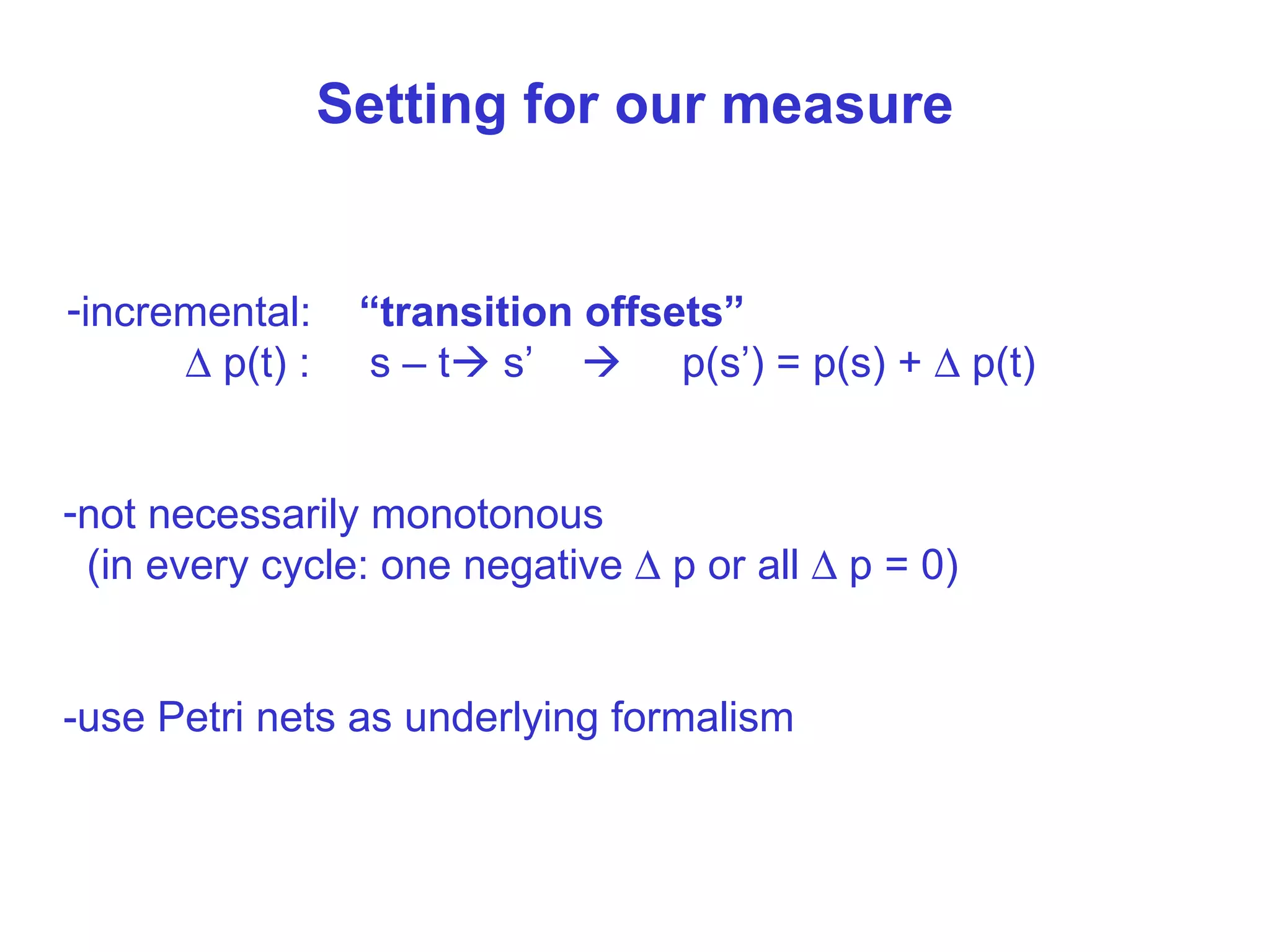
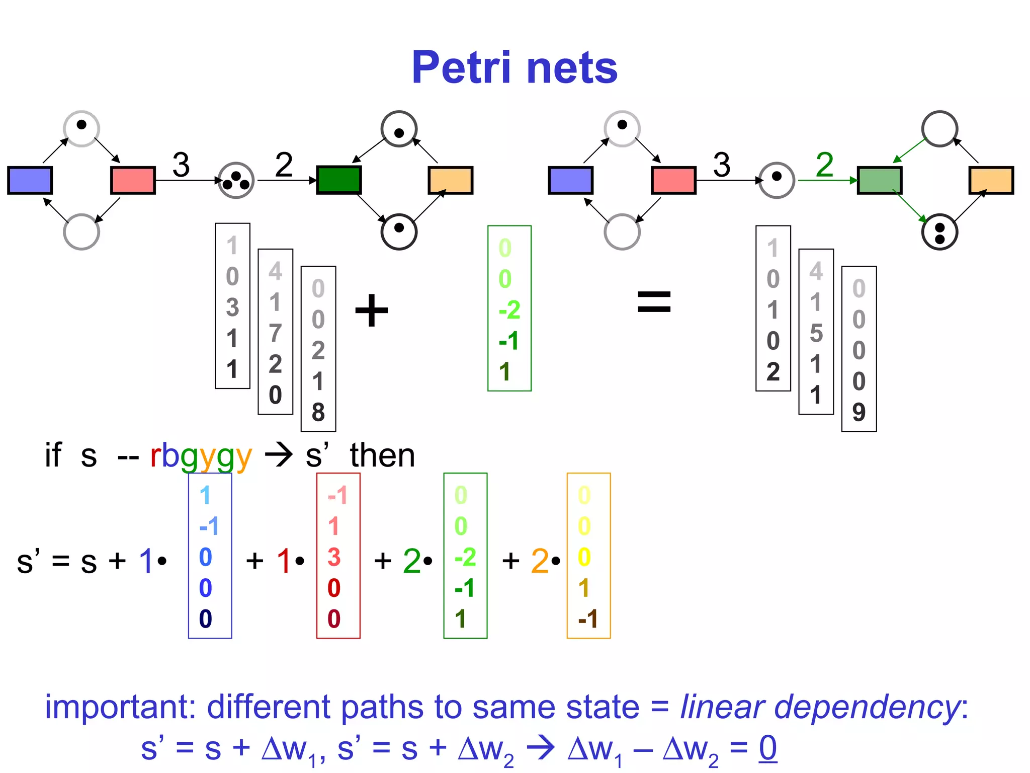
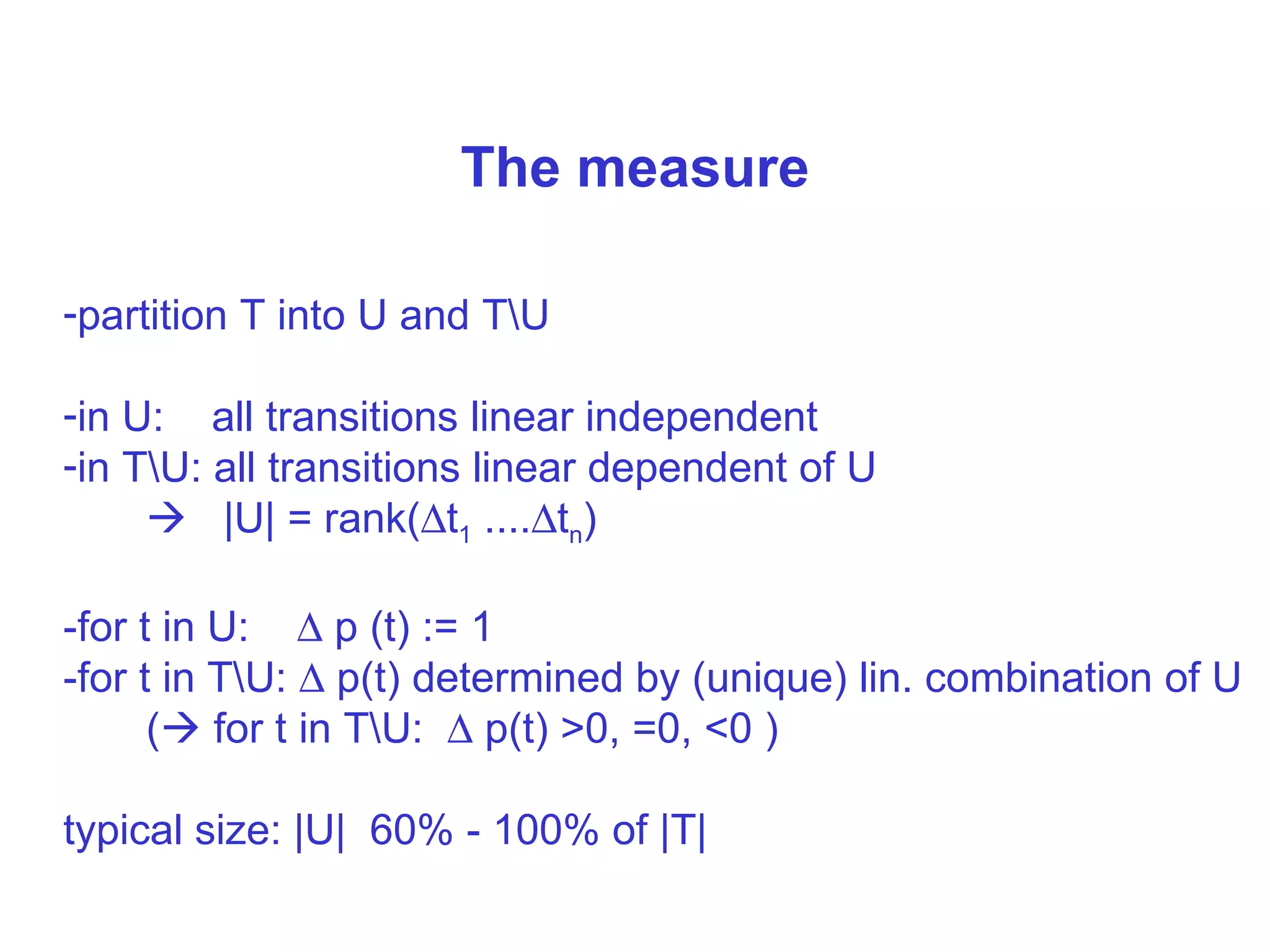
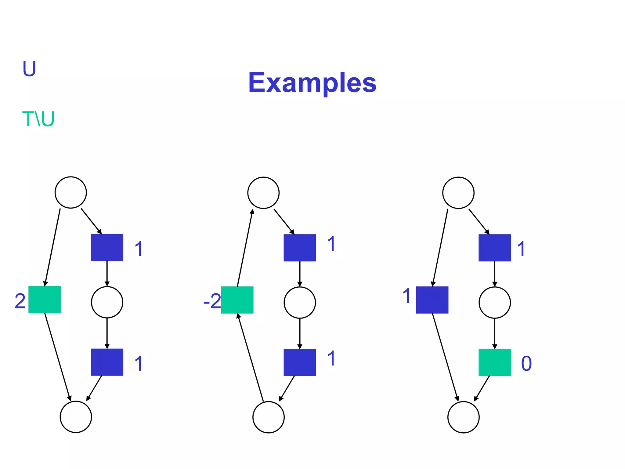
The document discusses calculating a progress measure for the sweep-line method of model checking. The sweep-line method works by assigning each state a progress value such that progress increases along transitions. However, progress is not always monotonic. The document proposes calculating incremental transition offsets to define progress such that it is not necessarily monotonic but increases overall. It describes partitioning transitions into independent and dependent sets and assigning offsets of 1 and determined combinations respectively to define the progress measure. This captures progress while addressing non-monotonicity in a way that is typically efficient.

1. Automated calculation of a progress measure for the sweep-line method Karsten Schmidt Humboldt-Universit ät zu Berlin

2. Sometime it’s good to forget... A) store only important states - branching - cover all cycles B) throw away if they cease to be useful (*) - the sweep-line method [Mailund] (*) by help of a progress measure

3. Road map The sweep-line method (basic/extended) Calculation of a progress measure Discussion - Combination with other reduction techniques

4. The sweep-line method (Basic) Idea: state s  progress value p(s) with s -t  s’  p(s)  p(s’) Not yet seen  Processed p Unprocessed sweep-line

5. The sweep-line method (extended) If p is not monotonous: s s’ p(s’) < p(s) Consequently: not too often p(s’) < p(s) t mark s’ “persistent” start new sweep from s’

6. Setting f or our measure incremental: “transition offsets”  p(t) : s – t  s’  p(s’) = p(s) +  p(t) not necessarily monotonous (in every cycle: one negative  p or all  p = 0) -use Petri nets as underlying formalism

7. Petri nets 1 0 3 1 1 1 0 1 0 2 if s -- r b g y g y  s’ then important: different paths to same state = linear dependency : s’ = s +  w 1 , s’ = s +  w 2   w 1 –  w 2 = 0 3 2 3 2 0 0 -2 -1 1 + = s’ = s + 1 • + 1 • + 2 • + 2 • 1 -1 0 0 0 -1 1 3 0 0 0 0 0 1 -1 0 0 -2 -1 1 4 1 7 2 0 0 0 2 1 8 4 1 5 1 1 0 0 0 0 9

8. The measure partition T into U and T\U in U: all transitions linear independent in T\U: all transitions linear dependent of U  |U| = rank(  t 1 ....  t n ) -f or t in U:  p (t) := 1 -f or t in T\U:  p(t) determined by (unique) lin. combination of U (  f or t in T\U:  p(t) >0, =0, <0 ) typical siz e: |U| 60% - 100% of |T|

9. Examples U T\U 1 1 1 1 1 1 2 -2 0

10. Geometric interpretation p 2 p 1 p 3 s U progress p(s) 1

11. Possible optimizations F or t in U: other values than 1 Optimization problem open: do heuristics help (simulated annealing, hill climbing...)? Choice of U e.g. small “regress edge connectedness” (checking all options = combinatorial explosion)

12. Combination with Partial Order Reduction simple versions (ample set determined by current state) work deadlocks, reachability,... advances versions (add., graph structure investigated) do not LTL, CTL

13. Combination with Symmetry Problem: transform state s to canonical representative c(s) so far not guaranteed: p(s) = p(c(s)) ! Fortunately: Petri net symmetry induces equivalence on transitions s.t. more involved measure that assigns equal  p to equivalent transitions s 0 s t 1 t 2 ... t n c(s) t 1 ’ t 2 ’... t n ’ t i equivalent t i ’

14. Availability www.informatik.hu-berlin.de/~kschmidt/lola.html also: integrated into The Model Checking Kit (University of Stuttgart)