ASTM E 1049-85 Standard Practice for Cycle Counting in Fatigue Analysis

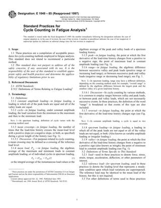
1. Designation: E 1049 – 85 (Reapproved 1997)
AMERICAN SOCIETY FOR TESTING AND MATERIALS
100 Barr Harbor Dr., West Conshohocken, PA 19428
Reprinted from the Annual Book of ASTM Standards. Copyright ASTM
Standard Practices for
Cycle Counting in Fatigue Analysis1
This standard is issued under the fixed designation E 1049; the number immediately following the designation indicates the year of
original adoption or, in the case of revision, the year of last revision. A number in parentheses indicates the year of last reapproval. A
superscript epsilon (e) indicates an editorial change since the last revision or reapproval.
1. Scope
1.1 These practices are a compilation of acceptable proce-dures
for cycle-counting methods employed in fatigue analysis.
This standard does not intend to recommend a particular
method.
1.2 This standard does not purport to address all of the
safety concerns, if any, associated with its use. It is the
responsibility of the user of this standard to establish appro-priate
safety and health practices and determine the applica-bility
of regulatory limitations prior to use.
2. Referenced Documents
2.1 ASTM Standards:
E 912 Definitions of Terms Relating to Fatigue Loading2
3. Terminology
3.1 Definitions:
3.1.1 constant amplitude loading—in fatigue loading, a
loading in which all of the peak loads are equal and all of the
valley loads are equal.
3.1.2 cycle—in fatigue loading, under constant amplitude
loading, the load variation from the minimum to the maximum
and then to the minimum load.
NOTE 1—In spectrum loading, definition of cycle varies with the
counting method used.
3.1.3 mean crossings—in fatigue loading, the number of
times that the load-time history crosses the mean-load level
with a positive slope (or a negative slope, or both, as specified)
during a given length of the history (see Fig. 1).
3.1.3.1 Discussion—For purposes related to cycle counting,
a mean crossing may be defined as a crossing of the reference
load level.
3.1.4 mean load, Pm —in fatigue loading, the algebraic
average of the maximum and minimum loads in constant
amplitude loading, or of individual cycles in spectrum loading,
Pm 5 ~Pmax 1 Pmin!/2 (1)
or the integral average of the instantaneous load values or the
algebraic average of the peak and valley loads of a spectrum
loading history.
3.1.5 peak—in fatigue loading, the point at which the first
derivative of the load-time history changes from a positive to
a negative sign; the point of maximum load in constant
amplitude loading (see Fig. 1).
3.1.6 range—in fatigue loading, the algebraic difference
between successive valley and peak loads (positive range or
increasing load range), or between successive peak and valley
loads (negative range or decreasing load range); see Fig. 1.
NOTE 2—In spectrum loading, range may have a different definition,
depending on the counting method used; for example, “overall range” is
defined by the algebraic difference between the largest peak and the
smallest valley of a given load-time history.
3.1.6.1 Discussion—In cycle counting by various methods,
it is common to employ ranges between valley and peak loads,
or between peak and valley loads, which are not necessarily
successive events. In these practices, the definition of the word
“range” is broadened so that events of this type are also
included.
3.1.7 reversal—in fatigue loading, the point at which the
first derivative of the load-time history changes sign (see Fig.
1).
NOTE 3—In constant amplitude loading, a cycle is equal to two
reversals.
3.1.8 spectrum loading—in fatigue loading, a loading in
which all of the peak loads are not equal or all of the valley
loads are not equal, or both. (Also known as variable amplitude
loading or irregular loading.)
3.1.9 valley—in fatigue loading, the point at which the first
derivative of the load-time history changes from a negative to
a positive sign (also known as trough); the point of minimum
load in constant amplitude loading (see Fig. 1).
3.2 Definitions of Terms Specific to This Standard:
3.2.1 load—used in these practices to denote force, stress,
strain, torque, acceleration, deflection, or other parameters of
interest.
3.2.2 reference load—for spectrum loading, used in these
practices to denote the loading level that represents a steady-state
condition upon which load variations are superimposed.
The reference load may be identical to the mean load of the
history, but this is not required.
3.3 For other definitions of terms used in these practices
1 These practices are under the jurisdiction of ASTM Committee E-8 on Fatigue
and Fracture and are the direct responsibility of Subcommittee E08.04 on Structural
Applications.
Current edition approved Feb. 22, 1985. Published June 1985.
2 Discontinued, see 1986 Annual Book of ASTM Standards, Vol 03.01.
1

2. E 1049
FIG. 1 Basic Fatigue Loading Parameters
refer to Definitions E 912.
4. Significance and Use
4.1 Cycle counting is used to summarize (often lengthy)
irregular load-versus-time histories by providing the number of
times cycles of various sizes occur. The definition of a cycle
varies with the method of cycle counting. These practices cover
the procedures used to obtain cycle counts by various methods,
including level-crossing counting, peak counting, simple-range
counting, range-pair counting, and rainflow counting. Cycle
counts can be made for time histories of force, stress, strain,
torque, acceleration, deflection, or other loading parameters of
interest.
5. Procedures for Cycle Counting
5.1 Level-Crossing Counting:
5.1.1 Results of a level-crossing count are shown in Fig.
2(a). One count is recorded each time the positive sloped
portion of the load exceeds a preset level above the reference
load, and each time the negative sloped portion of the load
exceeds a preset level below the reference load. Reference load
crossings are counted on the positive sloped portion of the
loading history. It makes no difference whether positive or
negative slope crossings are counted. The distinction is made
only to reduce the total number of events by a factor of two.
5.1.2 In practice, restrictions on the level-crossing counts
are often specified to eliminate small amplitude variations
which can give rise to a large number of counts. This may be
accomplished by filtering small load excursions prior to cycle
counting. A second method is to make no counts at the
reference load and to specify that only one count be made
between successive crossings of a secondary lower level
associated with each level above the reference load, or a
secondary higher level associated with each level below the
reference load. Fig. 2(b) illustrates this second method. A
variation of the second method is to use the same secondary
level for all counting levels above the reference load, and
another for all levels below the reference load. In this case the
levels are generally not evenly spaced.
5.1.3 The most damaging cycle count for fatigue analysis is
derived from the level-crossing count by first constructing the
largest possible cycle, followed by the second largest, etc.,
until all level crossings are used. Reversal points are assumed
to occur halfway between levels. This process is illustrated by
Fig. 2(c). Note that once this most damaging cycle count is
obtained, the cycles could be applied in any desired order, and
this order could have a secondary effect on the amount of
damage. Other methods of deriving a cycle count from the
level-crossings count could be used.
5.2 Peak Counting:
5.2.1 Peak counting identifies the occurrence of a relative
maximum or minimum load value. Peaks above the reference
load level are counted, and valleys below the reference load
level are counted, as shown in Fig. 3(a). Results for peaks and
valleys are usually reported separately. A variation of this
method is to count all peaks and valleys without regard to the
reference load.
5.2.2 To eliminate small amplitude loadings, mean-crossing
peak counting is often used. Instead of counting all peaks and
valleys, only the largest peak or valley between two successive
mean crossings is counted as shown in Fig. 3(b).
5.2.3 The most damaging cycle count for fatigue analysis is
derived from the peak count by first constructing the largest
possible cycle, using the highest peak and lowest valley,
followed by the second largest cycle, etc., until all peak counts
are used. This process is illustrated by Fig. 3(c). Note that once
this most damaging cycle count is obtained, the cycles could be
applied in any desired order, and this order could have a
secondary effect on the amount of damage. Alternate methods
of deriving a cycle count, such as randomly selecting pairs of
peaks and valleys, are sometimes used.
5.3 Simple-Range Counting:
5.3.1 For this method, a range is defined as the difference
between two successive reversals, the range being positive
when a valley is followed by a peak and negative when a peak
is followed by a valley. The method is illustrated in Fig. 4.
Positive ranges, negative ranges, or both, may be counted with
this method. If only positive or only negative ranges are
counted, then each is counted as one cycle. If both positive and
negative ranges are counted, then each is counted as one-half
cycle. Ranges smaller than a chosen value are usually elimi-nated
before counting.
5.3.2 When the mean value of each range is also counted,
the method is called simple range-mean counting. For the
example of Fig. 4, the result of a simple range-mean count is
2

3. given in X1.1 in the form of a range-mean matrix.
5.4 Rainflow Counting and Related Methods:
5.4.1 A number of different terms have been employed in
the literature to designate cycle-counting methods which are
similar to the rainflow method. These include range-pair
counting (1, 2),3 the Hayes method (3), the original rainflow
method (4-6), range-pair-range counting (7), ordered overall
range counting (8), racetrack counting (9), and hysteresis loop
counting (10). If the load history begins and ends with its
maximum peak, or with its minimum valley, all of these give
identical counts. In other cases, the counts are similar, but not
generally identical. Three methods in this class are defined
here: range-pair counting, rainflow counting, and a simplified
method for repeating histories.
E 1049
5.4.2 The various methods similar to the rainflow method
may be used to obtain cycles and the mean value of each cycle;
they are referred to as two-parameter methods. When the mean
value is ignored, they are one-parameter methods, as are
simple-range counting, peak counting, etc.
5.4.3 Range-Pair Counting—The range-paired method
counts a range as a cycle if it can be paired with a subsequent
loading in the opposite direction. Rules for this method are as
follows:
5.4.3.1 Let X denote range under consideration; and Y,
previous range adjacent to X.
(1) Read next peak or valley. If out of data, go to Step 5.
(2) If there are less than three points, go to Step 1. Form
ranges X and Y using the three most recent peaks and valleys
that have not been discarded.
(3) Compare the absolute values of ranges X and Y.
(a) If X < Y, go to Step 1.
3 The boldface numbers in parentheses refer to the list of references appended to
these practices.
(a)—Level Crossing Counting
(b)—Restricted Level Crossing Counting
FIG. 2 Level-Crossing Counting Example
3

4. E 1049
(a)—Peak Counting
(b)—Mean Crossing Peak Counting
(c)—Cycles Derived from Peak Count of (a)
FIG. 3 Peak Counting Example
(b) If X $ Y, go to Step 4.
(4) Count range Y as one cycle and discard the peak and
valley of Y; go to Step 2.
(5) The remaining cycles, if any, are counted by starting at
the end of the sequence and counting backwards. If a single
range remains, it may be counted as a half or full cycle.
5.4.3.2 The load history in Fig. 4 is replotted as Fig. 5(a)
and is used to illustrate the process. Details of the cycle
counting are as follows:
(1) Y 5 |A-B|; X 5 |B-C|; and X > Y. Count |A-B| as one
cycle and discard points A and B. (See Fig. 5(b). Note that a
cycle is formed by pairing range A-B and a portion of range
B-C.)
(2) Y 5 |C-D|; X 5 |D-E|; and X < Y.
(3) Y 5 |D-E|; X 5 |E-F|; and X < Y.
(4) Y 5 |E-F|; X 5 |F-G|; and X > Y. Count |E-F| as one
cycle and discard points E and F. (See Fig. 5(c).)
(5) Y 5 |C-D|; X 5 |D-G|; and X > Y. Count |C-D| as one
cycle and discard points C and D. (See Fig. 5(d).)
(6) Y 5 |G-H|; X 5 |H-I|; and X < Y. Go to the end and count
backwards.
(7) Y 5 |H-I|; X 5 |G-H|; and X > Y. Count |H-I| as one cycle
and discard points H and I. (See Fig. 5(e).)
(8) End of counting. See the table in Fig. 5 for a summary of
the cycles counted in this example, and see Appendix X1.2 for
this cycle count in the form of a range-mean matrix.
5.4.4 Rainflow Counting:
5.4.4.1 Rules for this method are as follows: let X denote
range under consideration; Y, previous range adjacent to X; and
S, starting point in the history.
(1) Read next peak or valley. If out of data, go to Step 6.
(2) If there are less than three points, go to Step 1. Form
4

5. E 1049
FIG. 4 Simple Range Counting Example—Both Positive and Negative Ranges Counted
ranges X and Y using the three most recent peaks and valleys
that have not been discarded.
(3) Compare the absolute values of ranges X and Y.
(a) If X < Y, go to Step 1.
(b) If X $ Y, go to Step 4.
(4) If range Y contains the starting point S, go to Step 5;
otherwise, count range Y as one cycle; discard the peak and
valley of Y; and go to Step 2.
(5) Count range Y as one-half cycle; discard the first point
(peak or valley) in range Y; move the starting point to the
second point in range Y; and go to Step 2.
(6) Count each range that has not been previously counted as
one-half cycle.
5.4.4.2 The load history of Fig. 4 is replotted as Fig. 6(a)
and is used to illustrate the process. Details of the cycle
counting are as follows:
(1) S 5 A; Y 5 |A-B|; X 5 |B-C|; X > Y. Y contains S, that is,
point A. Count |A-B| as one-half cycle and discard point A;
S 5 B. (See Fig. 6(b).)
(2) Y 5 |B-C|; X 5 |C-D|; X > Y. Y contains S, that is, point
B. Count| B-C| as one-half cycle and discard point B; S 5 C.
(See Fig. 6(c).)
(3) Y 5 |C-D|; X 5 |D-E|; X < Y.
(4) Y 5 |D-E|; X 5 |E-F|; X < Y.
(5) Y 5 |E-F|; X 5 |F-G|; X > Y. Count |E-F| as one cycle
and discard points E and F. (See Fig. 6(d). Note that a cycle is
formed by pairing range E-F and a portion of range F-G.)
(6) Y 5 |C-D|; X 5 |D-G|; X > Y; Y contains S, that is, point
C. Count |C-D| as one-half cycle and discard point C. S 5 D.
(See Fig. 6(e).)
(7) Y 5 |D-G|; X 5 |G-H|; X < Y.
(8) Y 5 |G-H|; X 5 |H-I|; X < Y. End of data.
(9) Count |D-G| as one-half cycle, |G-H| as one-half cycle,
and| H-I| as one-half cycle. (See Fig. 6(f).)
(10) End of counting. See the table in Fig. 6 for a summary
of the cycles counted in this example, and see Appendix X1.3
for this cycle count in the form of a range-mean matrix.
5.4.5 Simplified Rainflow Counting for Repeating Histories:
5.4.5.1 It may be desirable to assume that a typical segment
of a load history is repeatedly applied. Here, once either the
maximum peak or minimum valley is reached for the first time,
the range-pair count is identical for each subsequent repetition
of the history. The rainflow count is also identical for each
subsequent repetition of the history, and for these subsequent
repetitions, the rainflow count is the same as the range-pair
count. Such a repeating history count contains no half cycles,
only full cycles, and each cycle can be associated with a closed
stress-strain hysteresis loop (4, 10-12). Rules for obtaining
such a repeating history cycle count, called “simplified rain-flow
counting for repeating histories” are as follows:
5.4.5.2 Let X denote range under consideration; and Y,
previous range adjacent to X.
(1) Arrange the history to start with either the maximum
peak or the minimum valley. (More complex procedures are
available that eliminate this requirement; see (Ref 12).
(2) Read the next peak or valley. If out of data, STOP.
5

6. E 1049
(a) (b)
(c) (d)
FIG. 5 Range-Pair Counting Example
(3) If there are less than three points, go to Step 2. Form
ranges X and Y using the three most recent peaks and valleys
that have not been discarded.
(4) Compare the absolute values of ranges X and Y.
(a) If X < Y, go to Step 2.
(b) If X $ Y, go to Step 5.
(5) Count range Y as one cycle; discard the peak and valley
of Y; and go to Step 3.
5.4.5.3 The loading history of Fig. 4 is plotted as a repeating
load history in Fig. 7(a) and is used to illustrate the process.
Rearranging the history to start with the maximum peak gives
Fig. 7(b), Reversal Points A, B, and C being moved to the end
of the history. Details of the cycle counting are as follows:
(1) Y 5 |D-E|; X 5 |E-F|; X < Y.
(2) Y 5 |E-F|; X 5 |F-G|; X > Y. Count | E-F| as one cycle
and discard points E and F. (See Fig. 7(c).) Note that a cycle
is formed by pairing range E-F and a portion of range F-G.
(3) Y 5 |D-G|; X 5 |G-H|; X < Y.
(4) Y 5 |G-H|; X 5 |H-A|; X < Y.
(5) Y 5 |H-A|; X 5 |A-B|; X < Y.
(6) Y 5 |A-B|; X 5 |B-C|; X > Y. Count |A-B| as one cycle
and discard points A and B. (See Fig. 7(d).)
(7) Y 5 |G-H|; X 5 |H-C|; X < Y.
(8) Y 5 |H-C|; X 5 |C-D|; X > Y. Count |H-C| as one cycle
and discard points H and C. (See Fig. 7(e).)
(9) Y 5 |D-G|; X 5 |G-D|; X 5 Y. Count| D-G| as one cycle
and discard points D and G. (See Fig. 7(f).)
(10) End of counting. See the table in Fig. 7 for a summary
of the cycles counted in this example, and see Appendix X1.4
for this cycle count in the form of a range-mean matrix.
6

7. E 1049
(c) (d)
(e) (f)
FIG. 6 Rainflow Counting Example
7

8. (a) (b)
(c) (d)
(e) (f)
FIG. 7 Example of Simplified Rainflow Counting for a Repeating History
APPENDIX
(Nonmandatory Information)
X1. RANGE-MEAN MATRIXES FOR CYCLE COUNTING EXAMPLES
X1.1 The Tables X1.1-X1.4 which follow correspond to the
cycle-counting examples of Figs. 4-7. In each case, the table is
a matrix giving the number of cycles counted at the indicated
combinations of range and mean. Note that these examples are
the ones illustrating (1) simple-range counting, (2) range-pair
counting, (3) rainflow counting, and (4) simplified rainflow
counting for repeating histories, which are the methods that can
be used as two-parameter methods.
E 1049
8

9. E 1049
TABLE X1.1 Simple Range-Mean Counting (Fig. 4)
REFERENCES
(1) Anonymous, “The Strain Range Counter,” VTO/M/416, Vickers-
Armstrongs Ltd. (now British Aircraft Corporation Ltd.), Technical
Office, Weybridge, Surrey, England, April 1955.
(2) Burns, A., “Fatigue Loadings in Flight: Loads in the Tailpipe and Fin
of a Varsity,” Technical Report C.P. 256, Aeronautical Research
Council, London, 1956.
(3) Hayes, J. E., “Fatigue Analysis and Fail-Safe Design,” Analysis and
Design of Flight Vehicle Structures, E. F. Bruhn, ed., Tristate Offset
Range
Units
Mean Units
−2.0 −1.5 −1.0 −0.5 0 + 0.5 + 1.0 + 1.5 + 2.0
10 ... ... ... ... ... ... ... ... ...
9 ... ... ... ... ... ... ... ... ...
8 ... ... ... ... 0.5 ... 0.5 ... ...
7 ... ... ... 0.5 ... ... ... ... ...
6 ... ... ... ... ... ... 0.5 ... 0.5
5 ... ... ... ... ... ... ... ... ...
4 ... ... 0.5 ... ... ... 0.5 ... ...
3 ... ... ... 0.5 ... ... ... ... ...
2 ... ... ... ... ... ... ... ... ...
1 ... ... ... ... ... ... ... ... ...
TABLE X1.2 Range-Pair Counting (Fig. 5)
Range
(units)
Mean (units)
−2.0 −1.5 −1.0 −0.5 0 + 0.5 + 1.0 + 1.5 + 2.0
10 ... ... ... ... ... ... ... ... ...
9 ... ... ... ... ... ... ... ... ...
8 ... ... ... ... ... ... 1 ... ...
7 ... ... ... ... ... ... ... ... ...
6 ... ... ... ... ... ... 1 ... ...
5 ... ... ... ... ... ... ... ... ...
4 ... ... ... ... ... ... 1 ... ...
3 ... ... ... 1 ... ... ... ... ...
2 ... ... ... ... ... ... ... ... ...
1 ... ... ... ... ... ... ... ... ...
TABLE X1.3 Rainflow Counting (Fig. 6)
Range
(units)
Mean (units)
−2.0 −1.5 −1.0 −0.5 0 + 0.5 + 1.0 + 1.5 + 2.0
10 ... ... ... ... ... ... ... ... ...
9 ... ... ... ... ... 0.5 ... ... ...
8 ... ... ... ... 0.5 ... 0.5 ... ...
7 ... ... ... ... ... ... ... ... ...
6 ... ... ... ... ... ... 0.5 ... ...
5 ... ... ... ... ... ... ... ... ...
4 ... ... 0.5 ... ... ... 1.0 ... ...
3 ... ... ... 0.5 ... ... ... ... ...
2 ... ... ... ... ... ... ... ... ...
1 ... ... ... ... ... ... ... ... ...
TABLE X1.4 Simplified Rainflow Counting for Repeating
Histories (Fig. 7)
Range
Units
Mean Units
−2.0 −1.5 −1.0 −0.5 0 + 0.5 + 1.0 + 1.5 + 2.0
10 ... ... ... ... ... ... ... ... ...
9 ... ... ... ... ... 1 ... ... ...
8 ... ... ... ... ... ... ... ... ...
7 ... ... ... ... ... 1 ... ... ...
6 ... ... ... ... ... ... ... ... ...
5 ... ... ... ... ... ... ... ... ...
4 ... ... ... ... ... ... 1 ... ...
3 ... ... ... 1 ... ... ... ... ...
2 ... ... ... ... ... ... ... ... ...
1 ... ... ... ... ... ... ... ... ...
9

10. Co., Cincinnati, OH, 1965, pp. C13-1 - C13-42.
(4) Matsuishi, M., and Endo, T., “Fatigue of Metals Subjected to Varying
Stress,” Paper presented to Japan Society of Mechanical Engineers,
Fukuoka, Japan, March 1968. See also Endo, T., et al., “Damage
Evaluation of Metals for Random or Varying Loading,” Proceedings of
the 1974 Symposium on Mechanical Behavior of Materials, Vol 1, The
Society of Materials Science, Japan, 1974, pp. 371–380.
(5) Anzai, H., and Endo, T., “On-Site Indication of Fatigue Damage Under
Complex Loading,” International Journal of Fatigue, Vol 1, No. 1,
1979, pp. 49–57.
(6) Endo, T., and Anzai, H., “Redefined Rainflow Algorithm: P/V Differ-ence
Method,” Japan Society of Materials Science, Japan, Vol 30, No.
328, 1981, pp. 89–93.
(7) van Dijk, G. M., “Statistical Load Data Processing,” Paper presented
at Sixth ICAF Symposium, Miami, FL, May 1971. See also NLR MP
71007U, National Aerospace Laboratory, Amsterdam, 1971.
(8) Fuchs, H. O., et al., “Shortcuts in Cumulative Damage Analysis,”
E 1049
Fatigue Under Complex Loading: Analyses and Experiments, Vol
AE-6, R. M. Wetzel, ed., The Society of Automotive Engineers, 1977,
pp. 145–162.
(9) Nelson, D. V., and Fuchs, H. O., “Predictions of Cumulative Fatigue
Damage Using Condensed Load Histories,” Fatigue Under Complex
Loading: Analyses and Experiments, Vol AE-6, R. M. Wetzel, ed., The
Society of Automotive Engineers, 1977, pp. 163–187.
(10) Richards, F. D., LaPointe, N. R., and Wetzel, R. M., “A Cycle
Counting Algorithm for Fatigue Damage Analysis,” Automotive
Engineering Congress, Paper No. 740278, Society of Automotive
Engineers, Detroit, MI, February 1974.
(11) Dowling, N. E.,“ Fatigue Failure Predictions for Complicated Stress-
Strain Histories,” Journal of Materials, ASTM, Vol 7, No. 1, March
1972, pp. 71–87.
(12) Downing, S. D., and Socie, D. F., “Simplified Rainflow Counting
Algorithms,” International Journal of Fatigue, Vol 4, No. 1, January
1982, pp. 31–40.
The American Society for Testing and Materials takes no position respecting the validity of any patent rights asserted in connection
with any item mentioned in this standard. Users of this standard are expressly advised that determination of the validity of any such
patent rights, and the risk of infringement of such rights, are entirely their own responsibility.
This standard is subject to revision at any time by the responsible technical committee and must be reviewed every five years and
if not revised, either reapproved or withdrawn. Your comments are invited either for revision of this standard or for additional standards
and should be addressed to ASTM Headquarters. Your comments will receive careful consideration at a meeting of the responsible
technical committee, which you may attend. If you feel that your comments have not received a fair hearing you should make your
views known to the ASTM Committee on Standards, 100 Barr Harbor Drive, West Conshohocken, PA 19428.
10