This document provides an overview of Aspen Polymers, a software package for modeling polymerization processes. It discusses Aspen Polymers tools for characterizing polymer components and their properties, modeling reaction kinetics, and building steady-state process flowsheets. The document also provides references for related documentation on using Aspen Polymers.


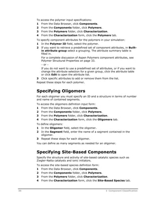


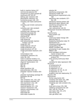
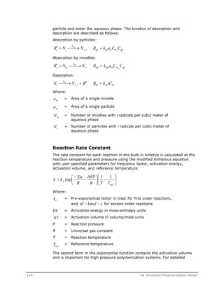
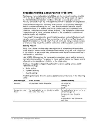
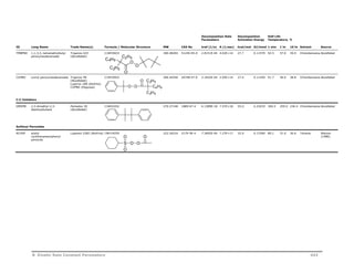
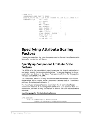
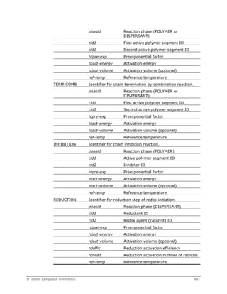
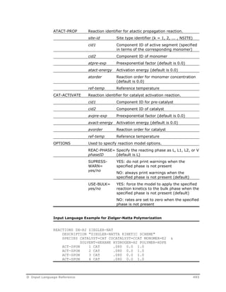
![Further, the assumption that polymer molecules are conserved once they are
formed can be invalid in the presence of certain side reactions, including
random (thermal) scission, which destroys polymer molecules, and chain
transfer to polymer, which causes inactive polymer molecules to become
active again, leading to long-chain branch formation and significantly
increasing the weight-average molecular weight and PDI. The molecular
weight distribution charts display the MWW and PDI calculated by the method
of moments and the method of instantaneous properties. If the predicted
values for the PDI are not in reasonable agreement with each other, it is most
likely due to these types of side reactions.
In the simplest case, linear polymerization in a single CSTR reactor, the ratios
of termination and chain transfer reaction rates to propagation reaction rates
are stored. The instantaneous chain length distribution is expressed as a
function of these ratios and chain length.
For the case of two CSTRs in series, at steady-state, the outlet polymer
distribution function is the weighted average of the distribution function in
each CSTR taken separately. The case of a plug flow reactor can be
approximated using multiple CSTRs, and similarly for a batch reactor.
By looking at the treatment of such reactor configurations, it can be deduced
that the final polymer distribution is a result of the entire system of reactors.
For this reason, the MWD implementation in Aspen Polymers needs to
consider the proper data structure to track distribution parameters at every
point in the flowsheet. Users should be able to request MWD from any point in
the flowsheet, and from this point the Aspen Plus flowsheet connectivity
information can be used to track polymerization history.
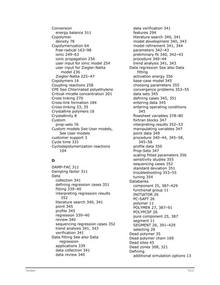
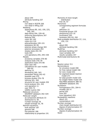
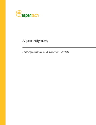
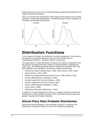
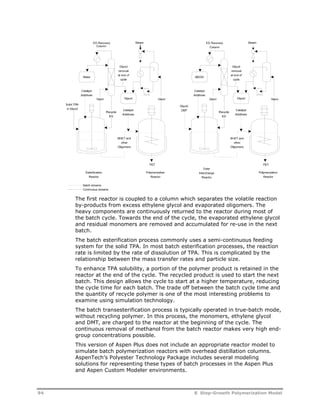
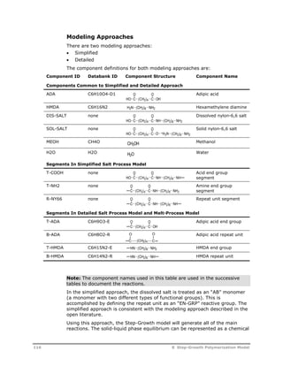
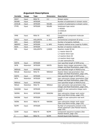
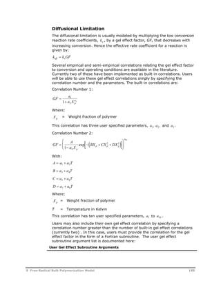
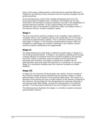
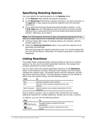
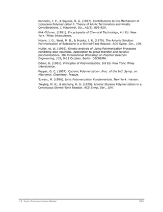
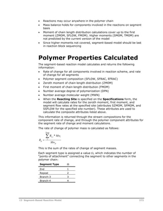
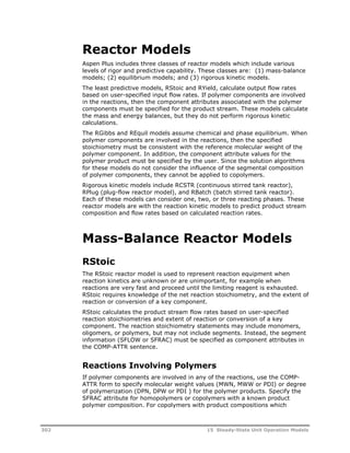
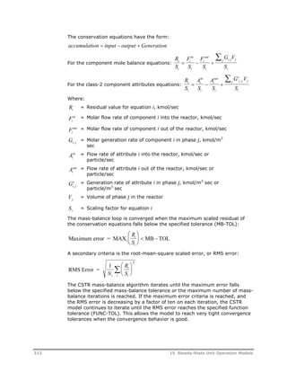
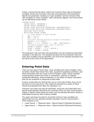
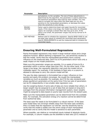
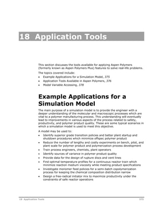
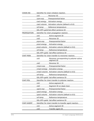
The calculation of chain length distribution for a batch reactor from reaction
rate parameters for linear addition polymerization was described by Hamielec
(Hamielec, 1992).
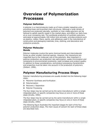
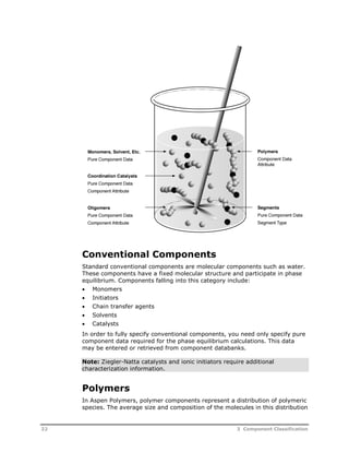
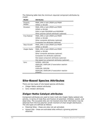
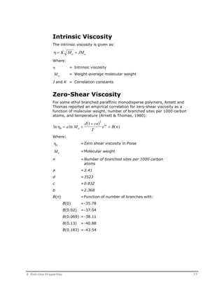
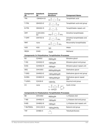
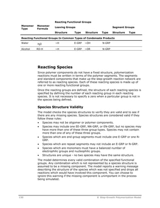
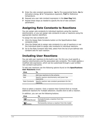
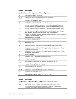
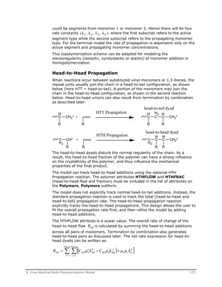
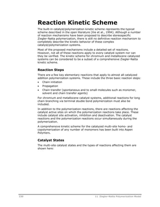
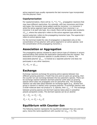
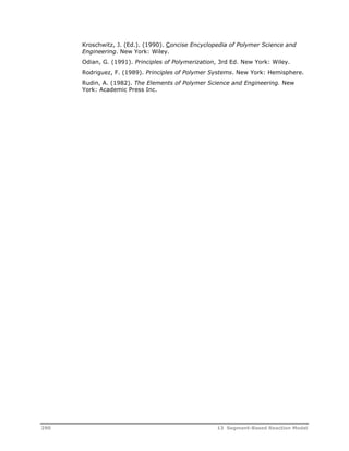
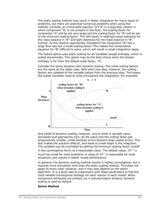
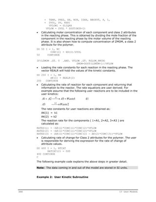
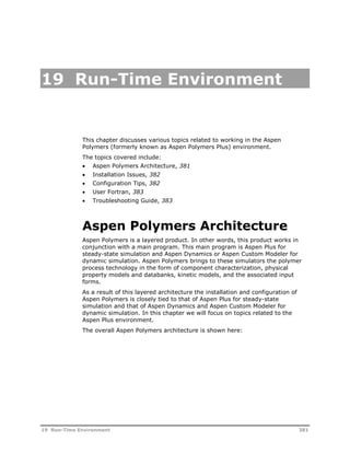
Consider the equations for the generation and consumption of free radicals. A
similar approach may be used for other active centers (Ziegler-Natta,
metallocene, etc.):
Radical Generation and Consumption Rates
R K [ M ][ R o
]
K [ T ][ R
o
]
I fm
fT
K [ M ] K [ M ] K [ T ] K
K [ R
o
]
p fm fT tc td
l
o
R
o
K M R
[ ][ 1]
p
r
K [ M ] K [ M ] K [ T ] K
K [ R
o
]
p fm fT tc td
r
o
R
Where:
R K f I I d 2 [ ] = Initiation rate
Instantaneous Distribution Parameters
Introducing two dimensionless parameters and .
5 Structural Property Distributions 61](https://image.slidesharecdn.com/aspenpolymersunitopsv82-usr-141128134016-conversion-gate02/85/Aspen-polymersunitopsv8-2-usr-73-320.jpg)
![
o
R
R
R
K R K M K T
[ ] [ ] [ ]
fm fT
p
K M
td f
p
td
[ ]
R
R
tc
p
o
K R
tc
K M
p
[ ]
[ ]
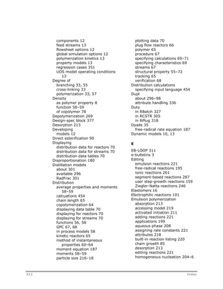
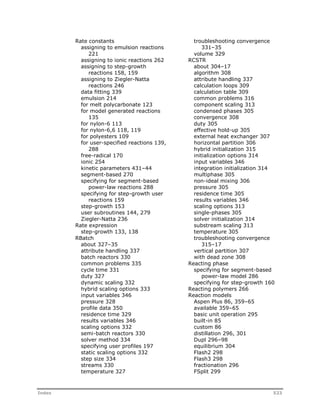
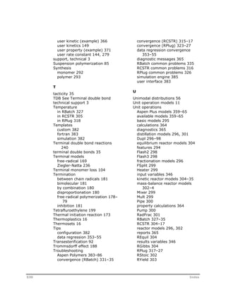
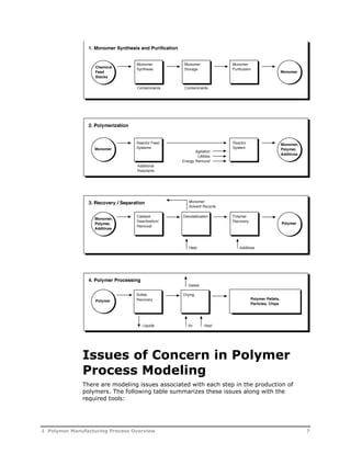
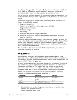
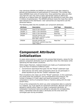
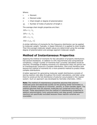
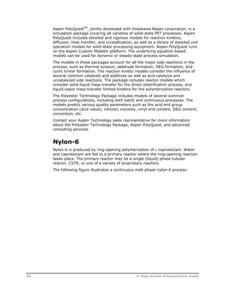
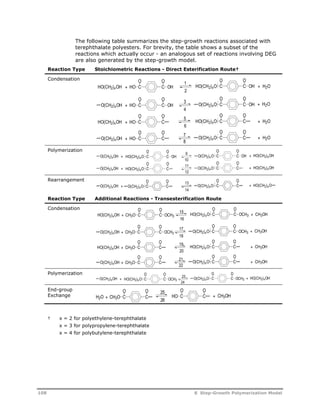
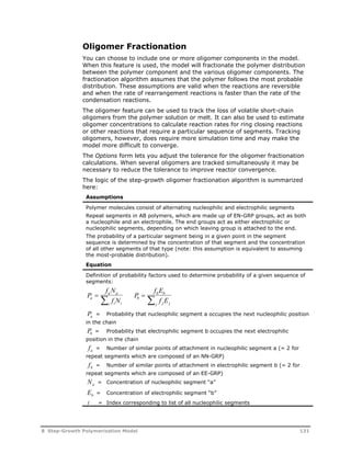
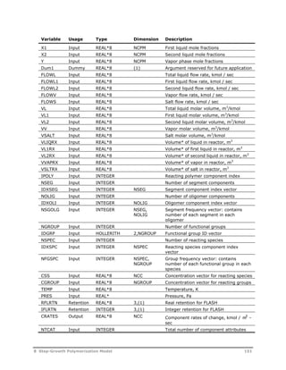
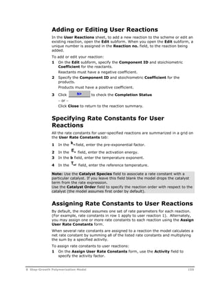
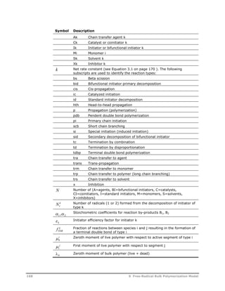
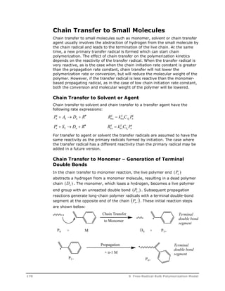
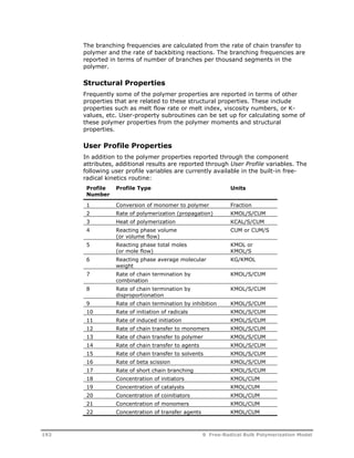
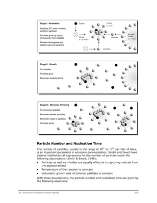
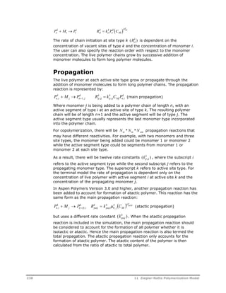
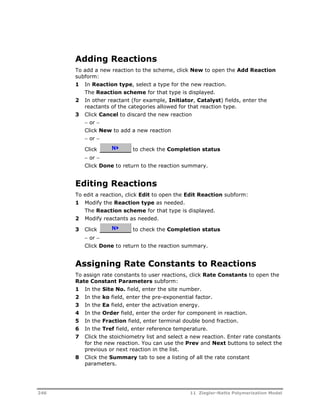
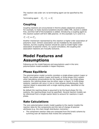
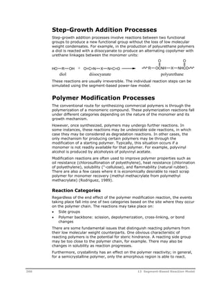
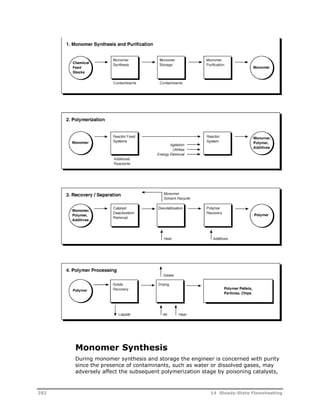
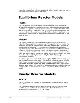
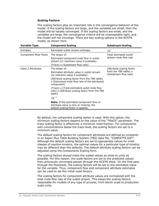
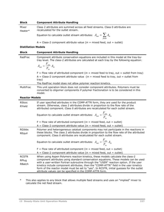
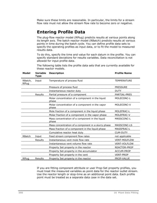
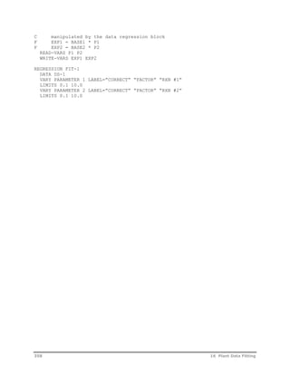
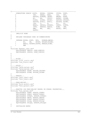
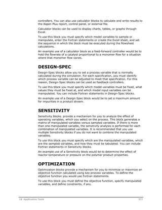
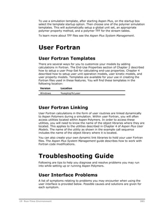
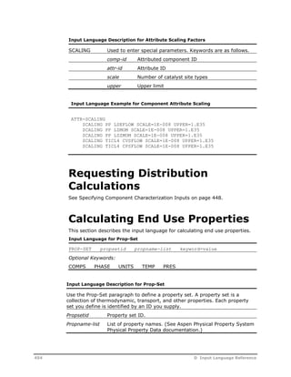
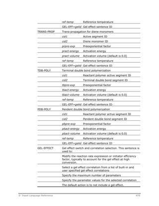
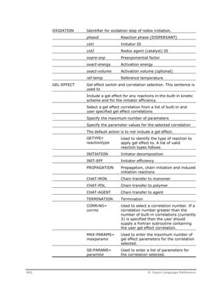
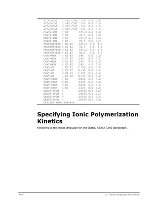
Where:
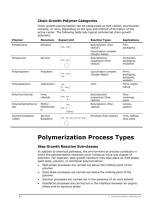
R K R M p p
[ o ][ ] = Propagation rate
R K R td td
[ o ]2 = Rate of termination by disproportionation
R K [ R o ]2 = Rate of termination by combination
tc tc
R K R M K R T f fm
[ o
][ ] [ o ][ ] = Total rate of chain transfer to
fT
small molecules (not
polymers)
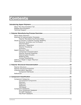
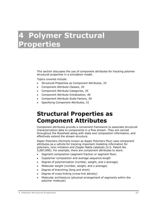
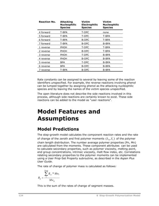
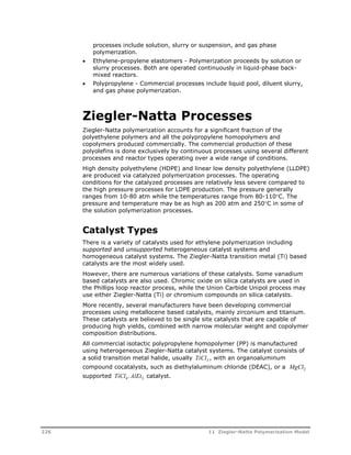
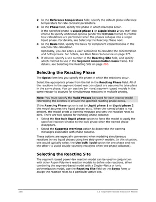
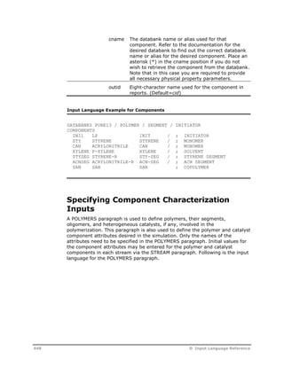
If we assume that the stationary-state hypothesis holds, then the initiation
rate is equal to the sum of the termination rates, RI Rtd Rtc .
The equations for the rate of generation and consumption of radicals can be
written as follows:
Ro R
l
1
o
1
Ro R o
r
r
1
1 Therefore:
Ro r
R
o r
Where:
1
1
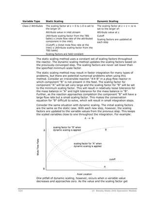
The rate of production of polymer molecules of chain length r , RFp (r) is
given by:
1 1
r
1
R ( r ) r
K M K T K R o R o
K R o
s
R
FP
r s
V
d V P
dt
fm fT td
r tc
2 s
1
o
Substituting [ ] Rf o
gives:
2
R r K R M r FP p
( ) o
1
r
62 5 Structural Property Distributions](https://image.slidesharecdn.com/aspenpolymersunitopsv82-usr-141128134016-conversion-gate02/85/Aspen-polymersunitopsv8-2-usr-74-320.jpg)


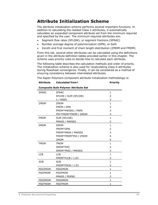
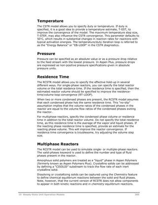
![Reaction
Type Reaction Stoichiometry
Acetaldehyde
Formation
Cyclic Trimer
Formation
O O
C C
O O
U5
O(CH2)2OH C C
O
OH + HCCH3
O
HCCH3
O O
O O
U6
O(CH2)2OH + OCH CH2 C C
C C +
O(CH2)2O
U7
U8
G T
HOT G T G T GH + H2O
T
G T
G
U9
U10
G T
HG T G T G T GH + HO(CH2)2OH
T
G T
G
U11
U12
G T
T
G T
G
G T G T G T GH O(CH2)2OH +
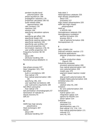
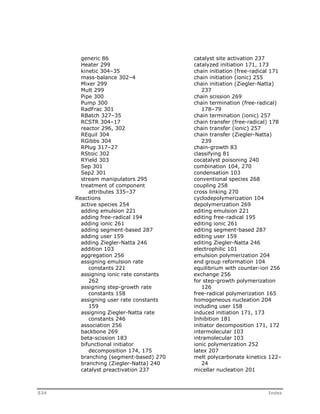
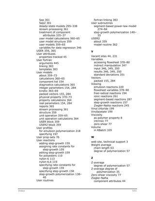
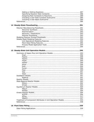
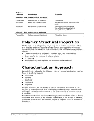
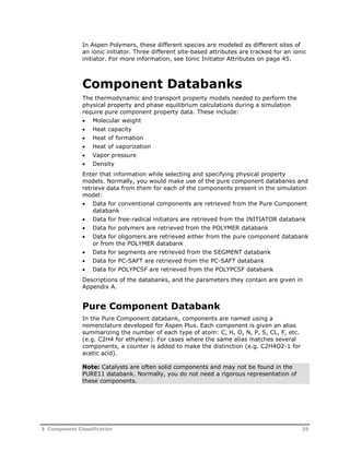
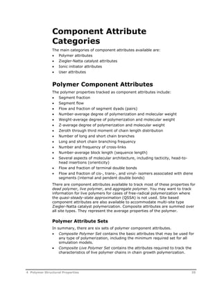
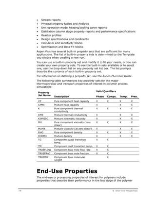
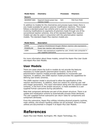
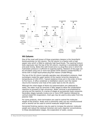
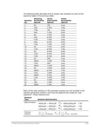
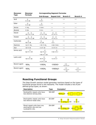
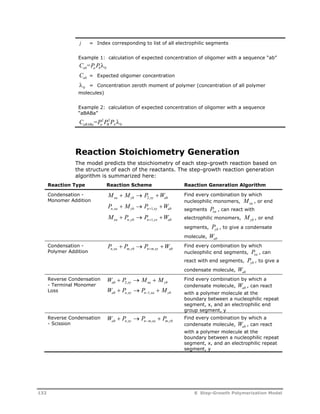
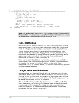
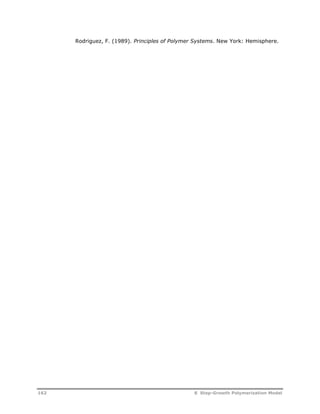
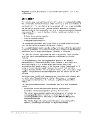
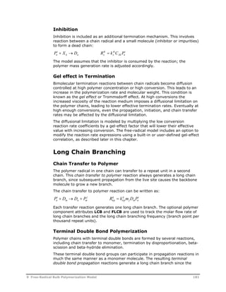
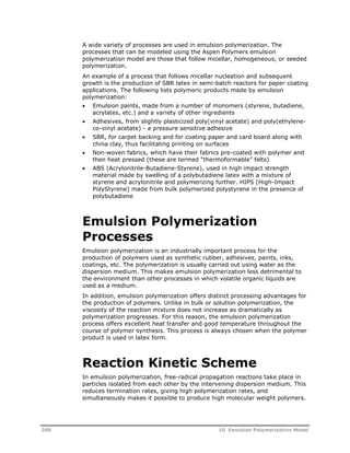
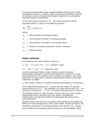
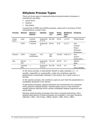
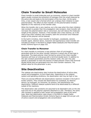
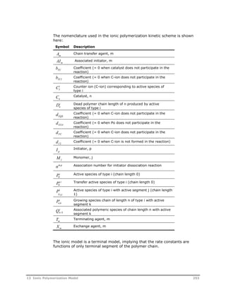
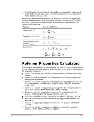
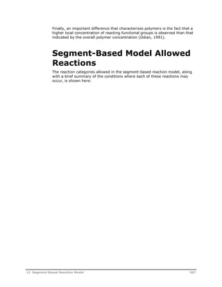
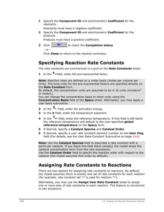
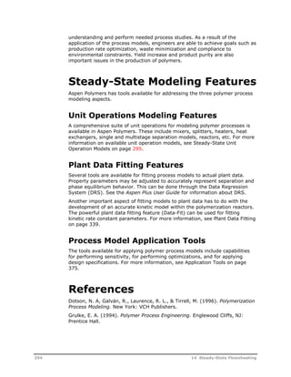
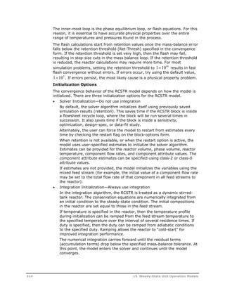
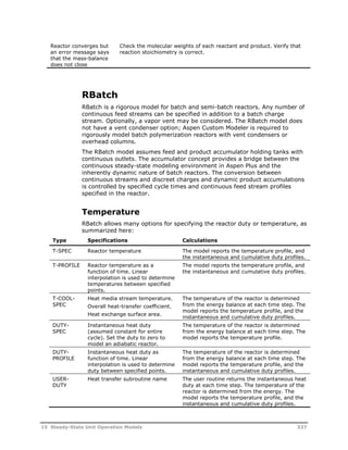
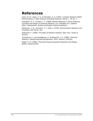
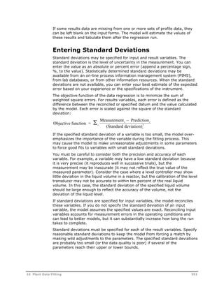
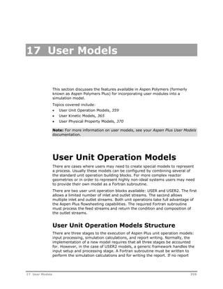
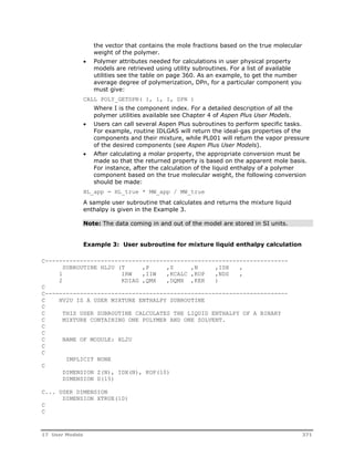
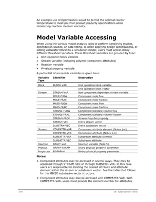
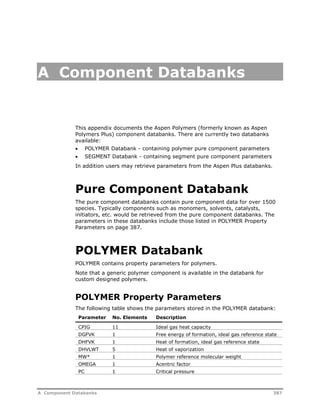
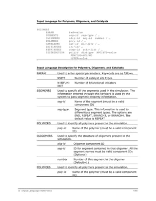
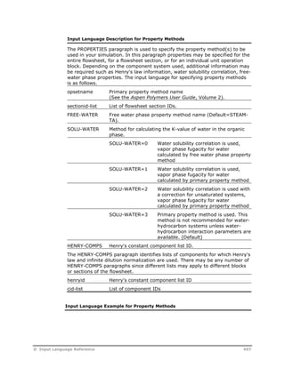
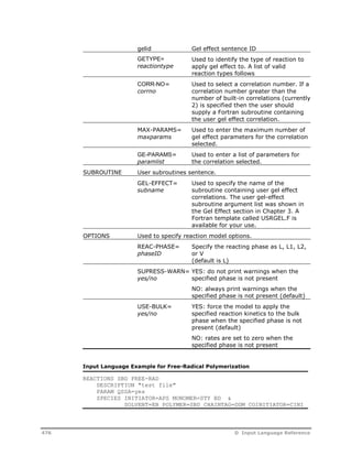
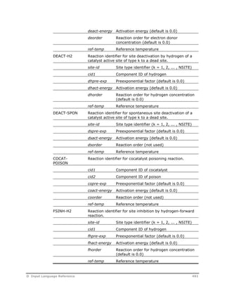
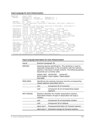
The recommended power-law exponents for the reactants in the side
reactions are:
Reaction
No. Power-Law Exponents; Modeling Notes
U1 EG = 2 (Multiply group-based pre-exponential factor by 4.0)
U2 EG = 1, T-EG = 1 (Multiply group-based pre-exponential factor by
2.0)
U3 T-EG = 2 (Multiply group-based pre-exponential factor by 1.0)
U4 Reaction is first order with respect to polyester repeat units, assume
concentration of repeat units is approximately equal to the
concentration of B-TPA, set power-law exponents B-TPA = 1.0 B-EG =
1x10⁻⁸
U5 T-EG = 1
U6 T-EG = 1, T-VINYL = 1
U7 Reaction is first order with respect to linear molecule with the
following segment sequence:
T-TPA: B-EG : B-TPA : B-EG : B-TPA : T-EG
option 1: assume this concentration = TPA concentration and use
power-law constant TPA = 1*
option 2: use the following equation, based on the most-probable
distribution, to estimate the concentration of this linear oligomer. This
equation can be implemented as a user-rate constant correlation
P
[ ] [ ] [ ] [ ] [ ] [ ] *[ ] *[
T EG
NUCL
B TPA
ELEC
2 2
B EG
NUCL
T TPA
ELEC
NUCL T EG T DEG B EG
2 2
2
2 0
ELEC T TPA B TPA
[ ] *[ ]
U8 H2O = 1, C3 = 1 (Multiply group-based pre-exponential factor by 6.0)
110 8 Step-Growth Polymerization Model](https://image.slidesharecdn.com/aspenpolymersunitopsv82-usr-141128134016-conversion-gate02/85/Aspen-polymersunitopsv8-2-usr-122-320.jpg)
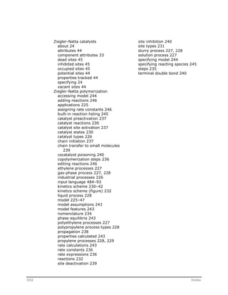
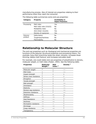
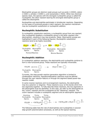
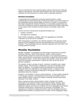
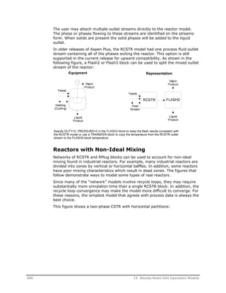
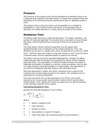
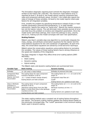
![Reaction
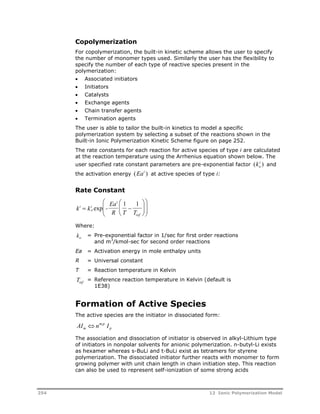
No. Power-Law Exponents; Modeling Notes
U9 Reaction is first order with respect to linear molecule with the
following segment sequence:
T-EG : B-TPA : B-EG : B-TPA : B-EG : B-TPA : T-EG
option 1: assume this concentration = TPA concentration and use
power-law constant TPA = 1*
option 2: use the following equation, based on the most-probable
distribution, to estimate the concentration of this linear oligomer. This
equation can be implemented as a user-rate constant correlation
P
[ ] [ ] [ ] [ ] [ ] *[ ] *[ ]
T EG
NUCL
2 3 2
B TPA
ELEC
B EG
NUCL
NUCL T EG T DEG B EG B DEG
2 2
2
2 0
ELEC T TPA B TPA
[ ] *[ ]
U10 EG = 1, C3 = 1 (Multiply group-based pre-exponential factor by 12.0)
U11 Reaction is first order with respect to linear molecule with the
following segment sequence:
~B-EG : B-TPA : B-EG : B-TPA : B-EG : B-TPA : T-EG
option 1: assume this concentration = T-EG concentration and use
power-law constant T-EG = 1*
option 2: use the following equation, based on the most-probable
distribution, to estimate the concentration of this linear oligomer. This
equation can be implemented as a user-rate constant correlation
P
[ ] [ ] [ ] [ ] [ ] *[ ] *[ ]
T EG
NUCL
B TPA
ELEC
3 3
B EG
NUCL
NUCL T EG T DEG B EG B DEG
2 2
2
2 0
ELEC T TPA B TPA
[ ] *[ ]
U12 T-EG = 1, C3 = 1 (Multiply group-based pre-exponential factor by
6.0)
* To avoid numerical problems, set power-law exponents to 1108 for reactants
which do not appear in the rate expression
0 = Concentration zeroth moment, mol/L (approximately=0.5*([T-TPA]+[T-EG]+[
T-DEG]+[T-VINYL])
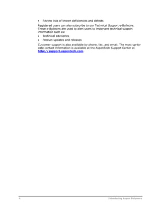
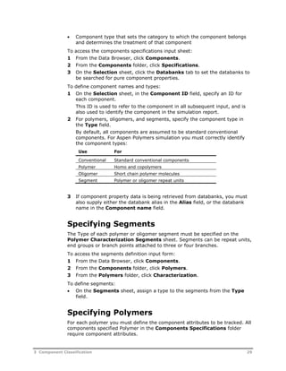
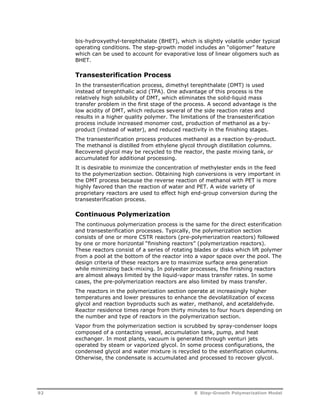
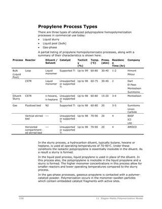
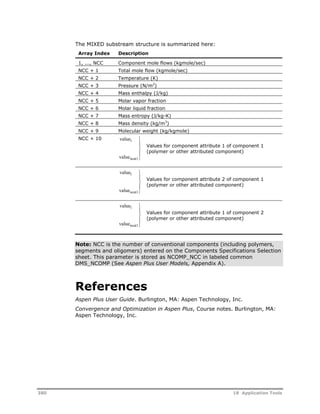
Nylon-6 Reaction Kinetics
Nylon-6 melt-phase polymerization reactions are initialized by the hydrolytic
scission of caprolactam rings. The reaction between water and caprolactam
generates aminocaproic acid. The reaction kinetics in the primary reactor are
sensitive to the initial water concentration.
The carboxylic and amine end groups of the aminocaproic acid molecules
participate in condensation reactions, releasing water and forming polymer
molecules. The resulting acid and amine end groups in the polymer react with
each other and with aminocaproic acid, releasing more water.
The amine end of aminocaproic acid and amine ends in polymer react with
caprolactam through ring addition. This reaction is the primary growth
mechanism in the nylon-6 process.
8 Step-Growth Polymerization Model 111](https://image.slidesharecdn.com/aspenpolymersunitopsv82-usr-141128134016-conversion-gate02/85/Aspen-polymersunitopsv8-2-usr-123-320.jpg)


![Reaction
No. Power-Law Exponents; Modeling Notes
U2 reverse Reaction is first order with respect to linear dimer P2 with the following segment
sequence:
T-NH2 :T-COOH
option 1: assume P2 concentration = ACA concentration and use power-law constant
ACA = 1*
option 2: use the following equation, based on the most-probable distribution, to
estimate concentration of P2 The denominator in this equation can be implemented
as a user rate constant, with first-order power-law constants for T-NH2 and T-COOH.
P
[ T
NH
2
]
[
]
2 T NH R NY
T COOH R NY 0
T COOH
[ ] [ ]
2 6 6
[ ] [
]
U3 forward ACA = 1, CL = 1
U3 reverse See U2 reverse reaction
U4 forward T-NH2 = 1, CL = 1
U4 reverse T-NH2 = 1 (this approximation assumes most T-NH2 end groups are attached to
repeat units)*
U5 forward ACA = 1, CD = 1
U5 reverse Reaction is first order with respect to linear trimer P3 with the following segment
sequence:
T-NH2 : R-NY6 : T-COOH
option 1: assume P3 concentration = ACA concentration and use power-law constant
ACA = 1*
option 2: use the following equation, based on the most-probable distribution, to
estimate concentration of P3 The denominator in this equation can be implemented
as a user rate constant, with first-order power-law constants for T-NH2, R-NY6, and
T-COOH.
[ T
NH
2
]
[ 6
]
P
[
]
2 T NH R NY
T COOH R NY 0
R NY
T COOH R NY
T COOH
[ 2 ] [ 6
]
[ ] [ ]
6 6
[ ] [
]
U6 forward T-NH2 = 1, CD = 1
U6 reverse T-NH2 = 1 (this approximation assumes most T-NH2 end groups are attached to
repeat units)*
*
To avoid numerical problems, set power-law exponents to 1108 for reactants which do not
appear in the rate expression
0 = Concentration zeroth moment, mol/L (approximately = 0.5 * ([T-COOH] + [T-NH2])
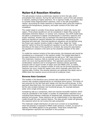
The side reactions are thought to be catalyzed by acid end groups in
aminocaproic acid and the polymer. A first-order power-law coefficient can be
used to account for the influence of the acid groups in these components.
Alternately, a user rate-constant subroutine can be developed to account for
the influence of the acid end groups.
Note that the forward and reverse terms of the reversible side reactions must
be defined as two separate user reactions in the model.
114 8 Step-Growth Polymerization Model](https://image.slidesharecdn.com/aspenpolymersunitopsv82-usr-141128134016-conversion-gate02/85/Aspen-polymersunitopsv8-2-usr-126-320.jpg)


![Reaction
No. Power-Law Exponents; Modeling Notes
U1 forward HMDA = 1, ADA = 1 Multiply group-based pre-exponential factor by 4.0
U1 reverse H2O = 1, DIS-SALT = 1
U2 forward DIS-SALT = 2
U2 reverse Reaction is first order with respect to water and polymer molecule P4 with the
following segment sequence:
T-HMDA : B-ADA : B-HMDA : T-ADA
option 1: assume P4 concentration = DIS-SALT concentration and use DIS-SALT =
1, H2O = 1*
option 2: set power-law exponent for H2O = 1 and use the following equation, based
on the most-probable distribution, to estimate concentration of P4 (this equation can
be implemented as a user rate constant).
0
P T ADA
4
B HMDA
2[
]
T HMDA B HMDA
[ ] 2[
]
T HMDA
[
]
T HMDA B HMDA
[ ] 2[ ]
[
]
T ADA B ADA
[ ] 2[
]
B ADA
2[
]
T ADA B ADA
[ ] 2[ ]
U3 forward DIS-SALT = 1, ADA = 1, multiply group rate constant by 2.0
U3 reverse Reaction is first order with respect to water and polymer molecule P 3,aa with the
following segment sequence:
T-ADA : B-HMDA : T-ADA
option 1: assume P 3,aa concentration = ADA concentration and use power-law
constants ADA = 1, H2O = 1*
option 2: set power-law exponent for H2O = 1 and use the following equation, based
on the most-probable distribution, to estimate concentration of P 3,aa (this equation
can be implemented as a user rate constant).
[ T
ADA
]
2
2
[ ]
P
3 aa T ADA B ADA
T HMDA B HMDA
B HMDA
, 2
2 0
[ ] [ ]
[ ] [ ]
U4 forward DIS-SALT = 1, HMDA = 1; multiply group rate constant by 2.0
U4 reverse Reaction is first order with respect to water and polymer molecule P 3,BB with the
following segment sequence:
T-HMDA : B-ADA : T-HMDA
option 1: assume P 3,BB concentration=HMDA concentration and use power-law
constants HMDA=1, H2O=1*
option 2: set power-law exponent for H2O = 1 and use the following equation, based
on the most-probable distribution, to estimate concentration of P 3,BB (this equation
can be implemented as a user rate constant).
[ T
HMDA
]
2
2
[ ]
P
3 aa T HMDA B HMDA
T ADA B ADA
B ADA
, 2
2 0
[ ] [ ]
[ ] [ ]
U5 forward DIS-SALT = 1, T-ADA = 1
U5 reverse H2O = 1, T-ADA = 1, set power law constants for B-ADA, B-HMDA to 1E-10 to avoid
numerical problems
U6 forward DIS-SALT = 1, T-HMDA = 1
120 8 Step-Growth Polymerization Model](https://image.slidesharecdn.com/aspenpolymersunitopsv82-usr-141128134016-conversion-gate02/85/Aspen-polymersunitopsv8-2-usr-132-320.jpg)
![Reaction
No. Power-Law Exponents; Modeling Notes
U6 reverse H2O = 1, T-ADA = 1, set power law constants for B-ADA, B-HMDA to 1E-10 to avoid
numerical problems
*
To avoid numerical problems, set power-law exponents to 1108 for reactants
which do not appear in the rate expression
0 = Concentration zeroth moment, mol/L (approximately = 0.5 * ([T-ADA] + [T-HMDA])
8 Step-Growth Polymerization Model 121](https://image.slidesharecdn.com/aspenpolymersunitopsv82-usr-141128134016-conversion-gate02/85/Aspen-polymersunitopsv8-2-usr-133-320.jpg)


![Symbol Description
[Nucl] Concentration of the attacking nucleophilic species, mol/L*
[Elec] Concentration of the attacking electrophilic species, mol/L*
fn
Number of electrophilic leaving groups in the attacking nucleophilic species.
This factor is 2 for diol and diamine monomers.
fe In reactions involving two victim species, fe is the number of electrophilic
groups in the electrophilic species. This factor is 2 for repeat units which
contain EE-GRP groups.
In reactions involving one victim species, fe is the number of nucleophilic
leaving groups in the electrophilic species. This factor is 2 for diacid, diester,
and carbonate monomers.
P In reactions involving two victim species, P is the probability of the victim
nucleophilic species being adjacent to the victim electrophilic species. This
probability factor is calculated by the model assuming the most probable
distribution:
P
f N
f N
vns vns
i i i
where:
fvns = Number of similar points of attachment in victim nucleophilic segment
(= 2 for NN-GRP repeat segments, 1 for all others)
Nvns = Concentration of victim nucleophilic segment
i = Index corresponding to list of all nucleophilic segments
i Index corresponding to the rate constant set number. The summation is
performed over the specified list of rate constant set numbers.
Symbol Description
Ci
Catalyst concentration for rate constant set i. If the catalyst species is
specified, this is the concentration of the species. If the catalyst group is
specified, this the group concentration. If both species and group are specified,
this is the concentration of the species times the number of the specified group
in the specified species. If the catalyst is not specified, this factor is set to one.
ko
Pre-exponential factor in user-specified inverse-time units*
Ea Activation energy in user-specified mole-enthalpy units (default =0)
b Temperature exponent (default = 0)
R Universal gas constant in units consistent with the specified activation energy
T Temperature, K
Tref
Optional reference temperature. Units may be specified, and they are
converted to K inside the model.
flag User flag for rate constant set i. This flag points to an element of the user rate
constant array.
U User rate constant vector calculated by the optional user rate constant
subroutine. The user flag indicates the element number in this array which is
used in a given rate expression. When the user flag is not specified, or when
the user rate constant routine is not present, this parameter is set to 1.0.
* The concentration basis may be changed to other units using the Concentration
basis field on the Options sheet or using the optional concentration basis
subroutine.
134 8 Step-Growth Polymerization Model](https://image.slidesharecdn.com/aspenpolymersunitopsv82-usr-141128134016-conversion-gate02/85/Aspen-polymersunitopsv8-2-usr-146-320.jpg)


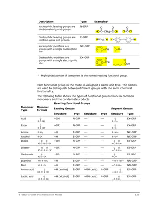
![User Reactions
The model cannot predict all types of reactions based on the specified
structures. Reactions which are not predicted by the model can be included as
user-specified reactions. These can include thermal scission reactions,
monomer or segment reformation, end-group modification, etc.
The user-specified reactions apply a modified power-law rate expression, as
shown here:
Equation
b
Ea
1 1
i
k Catalyst k e T
i
Tref specified i
net i i o i U flag
T
ref
R T T
ref
, [ ]
Ea
i
Tref unspecified i
k [ Catalyst ] k e RT b
iU flag
net ,
i i o i T Assign User Rate Constants is used: rate activity C a
mj k
m m j j i net ,
i
rate a
Assign User Rate Constants is not used: C mj k (m i) m j j
net ,
i
Nomenclature
Symbol Description
m User reaction number
i Rate constant set number
j Component number
Product operator
Cj
Concentration* of component j, mol/L
i
Catalyst order term for catalyst i (default = 1)
mj Power-law exponent for component j in reaction m
ko
Pre-exponential factor in user-specified inverse-time and concentration units*
net ,i k Net rate constant for set i
Ea Activation energy in user-specified mole-enthalpy units (default =0)
b Temperature exponent (default = 0)
R Universal gas constant in units consistent with the specified activation energy
T Temperature, K
Tref
Optional reference temperature. Units may be specified, they are converted to K in the
model.
flag User flag for rate constant set i. This flag points to an element of the user rate constant
array.
U User rate constant vector calculated by the optional user rate constant subroutine. The
user flag indicates the element number in this array which is used in a given rate
expression. When the user flag is not specified, or when the user rate constant routine
is not present, this parameter is set to 1.0.
138 8 Step-Growth Polymerization Model](https://image.slidesharecdn.com/aspenpolymersunitopsv82-usr-141128134016-conversion-gate02/85/Aspen-polymersunitopsv8-2-usr-150-320.jpg)


![Variable Usage Type Dimension Description
RCUSER Output REAL*8 NURC User rate constant vector (See User
Rate-Constant Subroutine, page 144)
CATWT Input REAL*8 Catalyst weight, kg (in RPLUG,
weight/length)
Example 3 illustrates how to use this subroutine to implement complex rate
expressions in the Step-Growth model.
Example 3: Implementing a Non-Ideal Rate Expression
Suppose a side reaction QZ is first order with respect to component Q and
first order with respect to a catalyst C. The effectiveness of the catalyst is
reduced by inhibitor I according to the following equation:
C
actual
1 ( )
C
eff a bT I
Where:
[C ] eff = Effective catalyst concentration, mol/L
[C ] actual = Actual catalyst concentration, mol/L
[I] = Inhibitor concentration, mol/L
T = Temperature, K
a,b = Equation parameters
The net rate expression can thus be written as:
C
a bT I
1 1
*
R T Tref
actual k e
rate Q
o
E
( )
[ ]
1
Where:
ko = Pre-exponential factor, (L/mol)/sec
E* = Activation energy
R = Gas law constant
Tref = Reference temperature for ko
[Q] = Concentration of component Q, mol/L
The standard rate expression for side reactions is:
E
R T T
1 1
*
rate k e ref C i
U j o
i
i
* ( )
Where:
= Product operator
Ci = Concentration of component i
8 Step-Growth Polymerization Model 147](https://image.slidesharecdn.com/aspenpolymersunitopsv82-usr-141128134016-conversion-gate02/85/Aspen-polymersunitopsv8-2-usr-159-320.jpg)
![i = Power-law exponent for component i
U = User rate constant
j = User rate-constant flag
Suppose the rate constant for the uninhibited reaction is 3 103 (L/mol)/min
at 150C, with an activation energy of 20 kcal/mol, and the inhibition rate
constants are A=0.20 L/mol, B=0.001 L/mol-K. The stoichiometric coefficients
and power-law exponents are specified directly in the Stoic and PowLaw-Exp
keywords. The Arrehnius rate parameters and reference temperature are also
specified directly in the model.
The parameters for the user rate constant equation can be specified using the
optional REALRC list. Including the parameters in the REALRC list allows the
model user to adjust these parameters using the standard variable accessing
tools, such as Sensitivity, Design-Specification, and Data-Regression.
The resulting model input is summarized below:
USER-VECS NREALRC=2 NUSERRC=1
REALRC VALUE-LIST=0.2D0 0.001D0
STOIC 1 Q -1.0 / Z 1.0
POWLAW-EXP 1 Q 1.0 / C 1.0
RATE-CON 1 3D-3<1/MIN> 20.000<kcal/mol>
TREF=150.0<C> URATECON=1
The power-law term from this equation is:
E
* 1 1
rate k e R T Tref
CQ o
Where:
[Q] = Concentration of component Q, mol/L
[C] = Catalyst concentration, mol/L
k= Pre-exponential factor
o Thus, the required user rate constant is:
1
U j
a bT I
( )
( ( )[ ]
1
1
Where:
[I] = Inhibitor concentration, mol/L
T = Temperature, K
a, b = Equation parameters
An excerpt from the user rate constant subroutine for this equation is shown
below:
C - Component Name -
INTEGER ID_IN(2)
DATA ID_IN /'INHI','BITO'/
148 8 Step-Growth Polymerization Model](https://image.slidesharecdn.com/aspenpolymersunitopsv82-usr-141128134016-conversion-gate02/85/Aspen-polymersunitopsv8-2-usr-160-320.jpg)
![C ======================================================================
C EXECUTABLE CODE
C ======================================================================
C - find location of inhibitor in the list of components -
DO 10 I = 1, NCOMP_NCC
IF ( IDSCC(1,I).EQ.ID_IN(1).AND.IDSCC(2,I).EQ.ID_IN(2) ) I_IN=I
10 CONTINUE
C - get the concentration of the inhibitor -
C_IN = 0.0D0
IF ( I_IN .GT.0 ) C_IN = CSS( I_IN )
C ----------------------------------------------------------------------
C Parameters: each REALR element defaults to zero if not specified
C ----------------------------------------------------------------------
A = 0.0D0
IF ( NREALR .GT. 0 ) A = REALR( 1 )
B = 0.0D0
IF ( NREALR .GT. 1 ) B = REALR( 2 )
C ----------------------------------------------------------------------
C User rate constant #1 U(1) = 1 / ( 1 + (A+BT)[I] )
C ----------------------------------------------------------------------
IF ( NURC.LT.1 ) GO TO 999
RCUSER(1) = 1.0D0 / ( 1.0D0 + ( A + B*TEMP ) * C_IN )
END IF
999 RETURN
User Kinetics Subroutine
The user kinetics subroutine is used to supplement the built-in kinetic
calculations. Use this subroutine when the side reaction kinetics are too
complicated to represent through the user rate constant routine, or when
previously written Fortran routines are to be interfaced to the Step-Growth
model.
The argument list for this subroutine is provided here. The argument list and
declarations are set up in a Fortran template called USRKIS.F, which is
delivered with Aspen Polymers.
User Subroutine Arguments
SUBROUTINE USRKIS(
1 SOUT, NSUBS, IDXSUB, ITYPE, XMW,
2 IDSCC, NPO, NBOPST, NIDS, IDS,
3 NINTB, INTB, NREALB, REALB,
4 NINTK, INTK, NREALK, REALK, NIWRK,
5 IWRK, NWRK, WRK, NCPMX, IDXM,
6 X, X1, X2, Y, DUMXS,
7 FLOWL, FLOWL1, FLOWL2, FLOWV, DUMFS,
8 VLQ, VLQ1, VLQ2, VVP, VOLSLT,
9 VLIQRX, VL1RX, VL2RX, VVAPRX, VSLTRX,
* IPOLY, NSEG, IDXSEG, NOLIG, IDXOLI,
1 NSGOLG, NGROUP, IDGRP, NSPEC, IDXSPC,
2 NFGSPC, CSS, CGROUP, TEMP, PRES,
3 RFLRTN, IFLRTN, CRATES, NTCAT, RATCAT,
4 NRC, PREEXP, ACTNRG, TEXP, TREF,
5 IUFLAG, NURC, RCUSER )
8 Step-Growth Polymerization Model 149](https://image.slidesharecdn.com/aspenpolymersunitopsv82-usr-141128134016-conversion-gate02/85/Aspen-polymersunitopsv8-2-usr-161-320.jpg)


![Symbol Description
f Initiator efficiency
[I] Initiator concentration in the aqueous phase (kmol/m3)
ka
Absorption constant for particles (s-1)
jcr Critical chain length
p
Volume fraction of polymer in polymer particle
kd
Initiator dissociation constant (s-1)
kde
Rate constant for the desorption of radicals from the
particles (m3/s)
kam
Rate constant for the absorption of radicals by micelles
(m/s)
kap
Rate constant for the absorption of radical by the particles
(m/s)
kp
Rate constant for propagation in particle phase (m3/kmol-s)
kpw
Rate constant for propagation in the aqueous phase
(m3/kmol-s)
kij Rate constant for activated initiation (m3/kmol-s)
act
kox
ij Rate constant for oxidation (m3/kmol-s)
kre
ij Rate constant for reduction (m3/kmol-s)
ktw
Rate constant for the termination in the aqueous phase
(m3/kmol-s)
pm Partition coefficient for the i-th component between polymer
Ki
particles and monomer droplets
Mp
Concentration of monomer in the polymer phase (kmol/m3)
Mwm
Molecular weight of monomer (kg/kmol)
Mw
Monomer concentration in aqueous phase (kmol/m3)
n Average number of radicals per particle
Np
Number of particles per unit volume of aqueous phase
(no./m3)
Na
Avogadro number
Nagg
Aggregation number
Nn
Number of particles containing n radicals per unit volume
(no./m3-s)
Rhomo
Rate of particle generation by homogeneous nucleation
(no./m3-s)
Rw
Radical concentration in the aqueous phase (kmol/m3)
RI
Rate of initiator dissociation (kmol/m3-s)
tnuc
Nucleation time(s)
v Volume of a single unswollen particle (m3)
10 Emulsion Polymerization Model 209](https://image.slidesharecdn.com/aspenpolymersunitopsv82-usr-141128134016-conversion-gate02/85/Aspen-polymersunitopsv8-2-usr-221-320.jpg)
![Symbol Description
vm
Volume of a single micelle (m3)
vh
Volume of a single particle formed by homogeneous
nucleation (m3)
v Volumetric growth rate of a single particle (m3/s)
vVolume of a swollen particle (m3)
s
vs Volumetric growth rate of a swollen particle (m3/s)
Rate of radical absorption by Np particles (Kmol/s)
Total rate of radical generation (Kmol/s- m3)
i
0
Zeroth moment of the particle size distribution (no./m3 of
aqueous phase)
1
First moment of the particle size distribution (m3/m3 of
aqueous phase)
2
Second moment of the particle size distribution (m6/m3 of
aqueous phase)
3
Third moment of the particle size distribution (m9/m3 of
aqueous phase)
Particles containing n radicals are produced by three kinetic events:
Absorption of a radical from the aqueous phase by a particle containing
(n-1) radical. The total rate of this event is given as:
N 1
p
nN
Radical desorption from a particle containing (n+1) radicals. The total rate
of this event is given as:
Nn+1 kde (n+1)
Termination in a particle containing (n+2) radicals. The total rate of this
reaction is given as:
[( 2)( 1)] 2 N k n n n tp
v
Particle Phase
Particles containing n free-radicals are depleted in the particle phase in three
analogous ways. By equating the rate of formation to the rate of depletion of
particles containing n free-radicals the recurrence formula is obtained:
/ ( 1)
N N N N k n N k n n
/ 1 ( 2)( 1) 1 1 2
n a p n de n tp N
210 10 Emulsion Polymerization Model
v
v
a
n a p de tp
a
N N N k n k n n
N
(3.12)
This recurrence formula was first developed by Smith and Ewart, in a slightly
modified form (Smith & Ewart, 1948). Equation 3.12 can be solved for the](https://image.slidesharecdn.com/aspenpolymersunitopsv82-usr-141128134016-conversion-gate02/85/Aspen-polymersunitopsv8-2-usr-222-320.jpg)


![In conventional emulsion polymerization where unimodal distributions are
normally encountered, the moments of the particle size distribution give
sufficient information about the nature of the particle size distribution. The
particle size distribution can be described in terms of different independent
variables such as diameter or volume of the particle. Since volumetric growth
rate of the particle in emulsion polymerization remains almost constant in
Stage I and Stage II of the process, the population balance equation is
formulated in terms of the volume of the particles.
General Population Balance Equation
The general population balance equation for the emulsion polymerization is
given as follows:
v , v F v
,
t
F t
t
k A N R R am m a w m h
v
v v v v
homo (3.15)
In Equation 3.15 the right-hand side represents the nucleation of particles
from miceller and homogeneous nucleation. Refer to the table on page 208
for an explanation of the variables used. The volumetric growth rate is v for
a single unswollen particle (Equation 3.5):
v
k M n
N
MW
d
p p
a
m
p
(3.16)
The general population balance equation can be converted to the equivalent
moment equations. The j-th moment of the particle size distribution is given
as:
( , )
0
jF j d
j
(3.17)
Applying moment definition in Equation 3.17 to the general population
balance equation in Equation 3.15, the first four moments of the particle size
distribution are given as:
d
dt
0 k A N [ R ] R am m a w
homo (3.18)
d
dt
v v k A N [ R ] v R (3.19)
0 m am m a w h
homo
1
d
dt
2v v2 k A N [ R ] v2 R m am m a w h
homo (3.20)
2
1
d
dt
3v v3 k A N [ R ] v3 R m am m a w h
homo (3.21)
3
2
Where:
kam = Kinetic constant for the absorption of the oligomeric
radicals into the micelles
Am = Area of the micelles
10 Emulsion Polymerization Model 217](https://image.slidesharecdn.com/aspenpolymersunitopsv82-usr-141128134016-conversion-gate02/85/Aspen-polymersunitopsv8-2-usr-229-320.jpg)


![Equation
b
Ea
1 1
i
k Catalyst k e T
i
Tref specified i
i
, [ ]
net i i o i U flag
T
ref
R T T
ref
Ea
i
Tunspecified * [ ] ref ,
i
k Catalyst i
e RT b
iU flag
net i i k o i T Assign User Rate Constants is used:
ratem
activitym C mj
k ,
aj
j i net i
ratem C k mj
,
aj
Assign User Rate Constants is not used: net m j
Nomenclature
Symbol Description
m User reaction number
i Rate constant set number
j Component number
Product operator
Cj
Concentration* of component j, mol/L
i
Catalyst order term for catalyst i (default = 1)
mj Power-law exponent for component j in reaction m
ko
Pre-exponential factor in user-specified inverse-time and concentration units**
net ,i k Net rate constant for set i assigned to reaction m
knet,m Net rate constant for reaction m
Ea Activation energy in user-specified mole-enthalpy units (default =0)
b Temperature exponent (default = 0)
R Universal gas constant in units consistent with the specified activation energy
T Temperature, K
Tref
Optional reference temperature. Units may be specified, they are converted to K in the
model. Defaults to global reference temperature (Global Tref) specified on the Specs sheet.
flag User flag for rate constant set i. This flag points to an element of the user rate constant
array.
U User rate constant vector calculated by the optional user rate constant subroutine. The user
flag indicates the element number in this array which is used in a given rate expression.
When the user flag is not specified, or when the user rate constant routine is not present,
this parameter is set to 1.0.
* The concentration basis may be changed to other units using the Concentration basis field on the
Specs sheet or using the optional concentration basis subroutine.
** The reference temperature may be specified globally on the Specs sheet or locally for each rate
constant set on the Rate-Constants sheet. If global and local reference temperatures are both
unspecified then this form of the equation is applied.
13 Segment-Based Reaction Model 271](https://image.slidesharecdn.com/aspenpolymersunitopsv82-usr-141128134016-conversion-gate02/85/Aspen-polymersunitopsv8-2-usr-283-320.jpg)


![[C ] eff = Effective catalyst concentration, mol/L
[C ] actual = Actual catalyst concentration, mol/L
[I] = Inhibitor concentration, mol/L
T = Temperature, K
a,b = Equation parameters
The net rate expression can thus be written as:
C
a bT I
1 1
*
R T Tref
actual k e
rate Q
o
E
( )
[ ]
1
Where:
ko = Pre-exponential factor, (L/mol)/sec
E* = Activation energy
R = Gas law constant
Tref = Reference temperature for ko
[Q] = Concentration of component Q, mol/L
The standard rate expression for side reactions is:
E
R T T
1 1
*
rate k e ref C i
U j o
i
i
* ( )
Where:
= Product operator
Ci = Concentration of component i
i = Power-law exponent for component i
U = User rate constant
j = User rate-constant flag
Suppose the rate constant for the uninhibited reaction is 3 103 (L/mol)/min
at 150C, with an activation energy of 20 kcal/mol, and the inhibition rate
constants are A=0.20 L/mol, B=0.001 L/mol-K. The stoichiometric coefficients
and power-law exponents are specified directly in the Stoic and PowLaw-Exp
keywords. The Arrehnius rate parameters and reference temperature are also
specified directly in the model.
The parameters for the user rate constant equation can be specified using the
optional REALRC list. Including the parameters in the REALRC list allows the
model user to adjust these parameters using the standard variable accessing
tools, such as Sensitivity, Design-Specification, and Data-Regression.
The resulting model input is summarized below:
USER-VECS NREALRC=2 NUSERRC=1
282 13 Segment-Based Reaction Model](https://image.slidesharecdn.com/aspenpolymersunitopsv82-usr-141128134016-conversion-gate02/85/Aspen-polymersunitopsv8-2-usr-294-320.jpg)
![REALRC VALUE-LIST=0.2D0 0.001D0
STOIC 1 Q -1.0 / Z 1.0
POWLAW-EXP 1 Q 1.0 / C 1.0
RATE-CON 1 3D-3<1/MIN> 20.000<kcal/mol>
TREF=150.0<C> URATECON=1
The power-law term from this equation is:
E
* 1 1
rate k e R T Tref
CQ o
Where:
[Q] = Concentration of component Q, mol/L
[C] = Catalyst concentration, mol/L
k= Pre-exponential factor
o Thus, the required user rate constant is:
1
U j
a bT I
( )
( ( )[ ]
1
1
Where:
[I] = Inhibitor concentration, mol/L
T = Temperature, K
a, b = Equation parameters
An excerpt from the user rate constant subroutine for this equation is shown
below:
C - Component Name -
INTEGER ID_IN(2)
DATA ID_IN /'INHI','BITO'/
C ======================================================================
C EXECUTABLE CODE
C ======================================================================
C - find location of inhibitor in the list of components -
DO 10 I = 1, NCOMP_NCC
IF ( IDSCC(1,I).EQ.ID_IN(1).AND.IDSCC(2,I).EQ.ID_IN(2) ) I_IN=I
10 CONTINUE
C - get the concentration of the inhibitor -
C_IN = 0.0D0
IF ( I_IN .GT.0 ) C_IN = CSS( I_IN )
C ----------------------------------------------------------------------
C Parameters: each REALR element defaults to zero if not specified
C ----------------------------------------------------------------------
A = 0.0D0
IF ( NREALR .GT. 0 ) A = REALR( 1 )
B = 0.0D0
IF ( NREALR .GT. 1 ) B = REALR( 2 )
C ----------------------------------------------------------------------
C User rate constant #1 U(1) = 1 / ( 1 + (A+BT)[I] )
C ----------------------------------------------------------------------
IF ( NURC.LT.1 ) GO TO 999
RCUSER(1) = 1.0D0 / ( 1.0D0 + ( A + B*TEMP ) * C_IN )
13 Segment-Based Reaction Model 283](https://image.slidesharecdn.com/aspenpolymersunitopsv82-usr-141128134016-conversion-gate02/85/Aspen-polymersunitopsv8-2-usr-295-320.jpg)


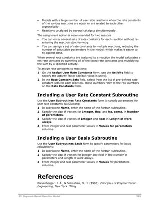


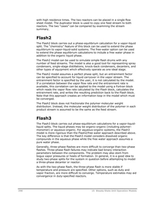


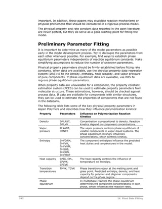


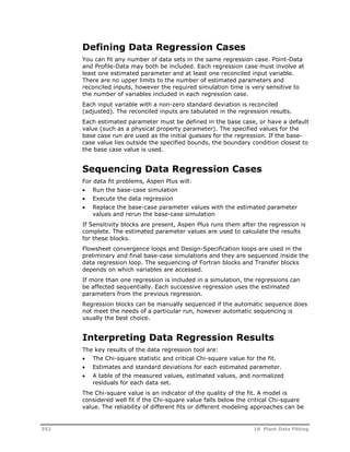


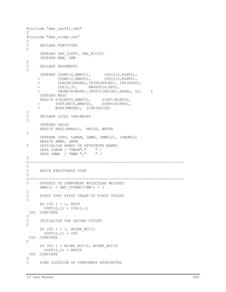


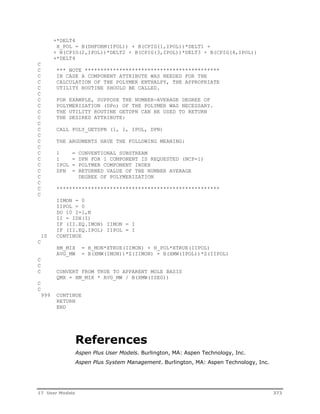


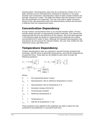

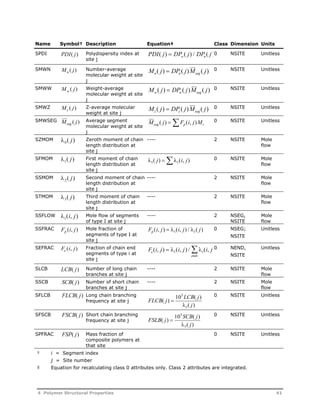
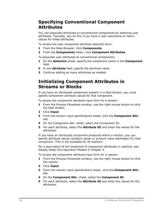
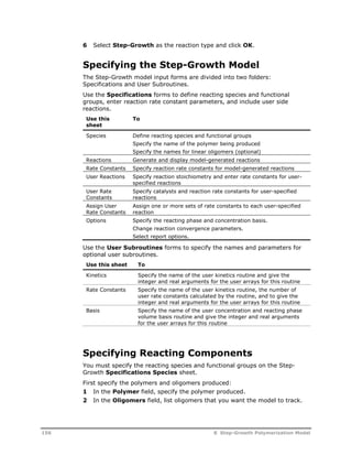
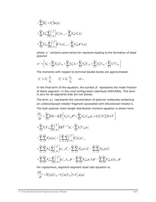
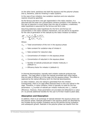
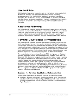
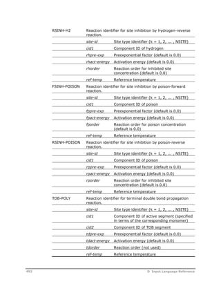
![Decomposition Rate
Parameters
Decomposition
Activation Energy
Half Life
Temperature, C
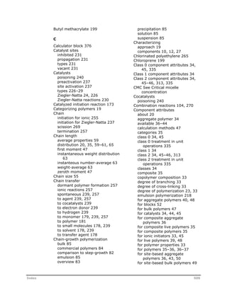
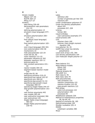
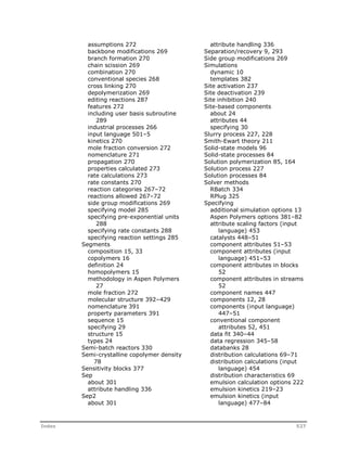
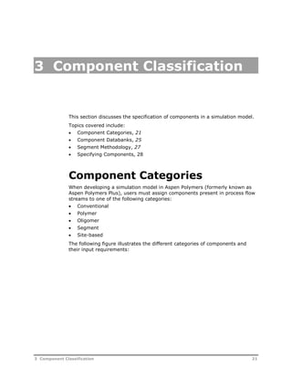
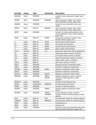
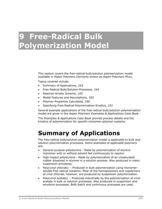
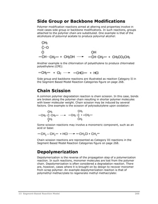
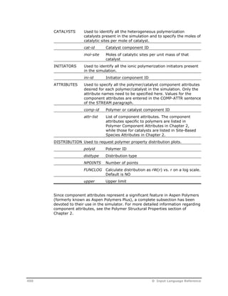
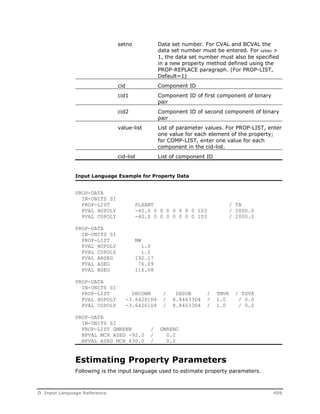
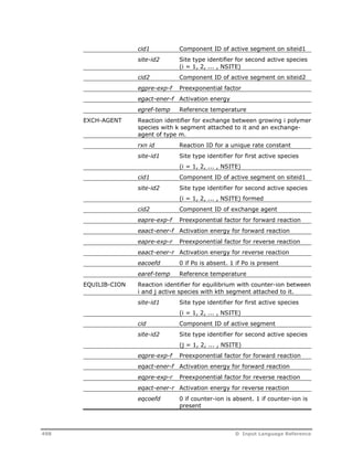
ID Long Name Trade Name(s) Formula / Molecular Structure MW CAS No kref (1/s) A (1/sec) kcal/mol GJ/kmol 1 min 1 hr 10 hr Solvent Source
Water Soluble Azo-Nitriles
ABAH 2,2’-azo-bis(2-
amidinopropane)
dihydrochloride
Vazo 56 (DuPont)
V-50 (Wako Chem)
C8H20N6Cl2 271.19264 2997-92-4 3.3436E-05 6.44E+14 29.4 0.12300 110.5 73.7 55.9 Water DuPont
VAZO68 4,4’-azo-bis
(4-cyanovaleric acid)
HCl NH HCl
HN
N N
H2N NH2
Vazo 68 (DuPont) C12H22N2O4 258.31776 2638-94-0 7.3642E-06 5.12E+12 27.2 0.11380 132.7 88.7 68.0 Water DuPont
VA61 2,2’-azo-bis[2-(2-
imidazolin-2-yl)propane]
N N
COOH
HOOC
VA-061 (Wako Chem) C12H22N6 250.34712 20858-12-2 1.3404E-03 1.00E+15 27.2 0.11400 78.4 45.0 28.9 Acidic water Wako
VA86 2,2’-Azobis[2-methyl-N-(2-
hydroxyethyl)propionamide]
N N
N
NH
N
HN
VA-086 C12H24N4O4 288.34712 61551-69-7 6.7869E-06 7.95E+14 30.6 0.12800 123.9 86.0 67.7 Water Wako
VAZO44 2,2’-azo-bis(N,N’-
dimethylene
isobutyramidine)
dihydrochloride
Vazo 44 (DuPont)
VA-44 (WakoChem)
O O
N N
HOH2CH2C NH HN CH2CH2OH
C12H24Cl2N6 323.26840 27776-21-2 1.3564E-04 8.10E+12 25.6 0.10700 103.3 63.0 44.0 Water DuPont
VA46B 2,2’-azo-bis[2-(2-
imidazolin-2-yl)propane
disulfate dihydrate
N N
N
NH
N
HN
2HCl
VA-046B (Wako Chem) C12H30N6O10S2 482.53664 20858-12-2 1.4388E-03 1.18E+17 30.4 0.12700 75.9 46.0 31.4 Water Wako
VA41 2,2’-azo-bis[2-(5-methyl-
2-imidazolin-2-yl)propane]
dihydrochloride
N N
N
NH
N H2SO4
HN
H2O
VA-041 (WakoChem) C14H26Cl2N6 349.30628 n/a 2.7035E-04 2.53E+15 28.9 0.12100 91.3 57.4 41.0 Water Wako
VA58 2,2’-azobis[2-(3,4,5,6-
tetrahydropyrimidin-2-
yl)propane] dihydrochloride
N N
N
NH
N
NH
HCl HCl
VA-058 (WakoChem) C14H28Cl2N6 351.32216 102834-39-0 2.5342E-05 1.44E+15 30.1 0.12600 111.8 75.5 58.0 Water Wako
VA57 2,2’-azobis[N-(2-
carboxyethyl)-2-
methylpropionamidine]
tetrahydrate
N N
NH
N N 2HCl
HN
VA-057 (WakoChem) C14H34N6O8 414.45960 n/a 2.8824E-05 5.56E+14 29.4 0.12300 112.0 74.9 57.0 Water Wako
HN
HN NH
HOOC COOH 4 H2O
N N
NH
434 B Kinetic Rate Constant Parameters](https://image.slidesharecdn.com/aspenpolymersunitopsv82-usr-141128134016-conversion-gate02/85/Aspen-polymersunitopsv8-2-usr-446-320.jpg)
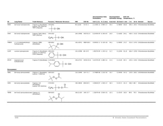
![Decomposition Rate
Parameters
Decomposition
Activation Energy
Half Life
Temperature, C
ID Long Name Trade Name(s) Formula / Molecular Structure MW CAS No kref (1/s) A (1/sec) kcal/mol GJ/kmol 1 min 1 hr 10 hr Solvent Source
VA85 2,2’-Azobis{2-methyl-N-[2-
(1-hydroxybuthyl)]
propionamide}
VA-085 (Wako Chem) C16H32N4O4 344.45464 n/a 7.8450E-07 6.41E+13 30.4 0.12700 148.2 105.4 85.0 Water Wako
VA60 2,2’-azo-bis{2-[1-(2-
hydroxyethyl)-2-imidazolin-
2-yl]propane}
dihydrochloride
O O
N N
NH HN
CH2CH3
H3CH2C
HOH2C CH2OH
VA-060 (Wako Chem) C16H32Cl2N6O2 411.37472 11858-13-0 1.9254E-05 9.56E+15 31.5 0.13200 111.7 76.9 60.0 Water Wako
Solvent Soluble Azo-Nitriles
N
N N
N N
N
2HCl
CH2CH2OH CH2CH2OH
V30 1-cyano-1-methyl-ethylazofomamide
V-30 (Wako Chem) C5H8N4O 140.14488 10288-28-5 4.4161E-08 1.86E+15 34.5 0.14430 164.9 123.9 104.0 Toluene Wako
AIBN 2,2'-azo-bis-isobutyronitrile Vazo 64 (DuPont)
Perkadox AIBN
(AkzoNobel)
CN
N N CONH2
C8H12N4 164.21024 78-67-1 1.0464E-05 2.74E+15 31.1 0.13023 118.3 82.0 64.4 Chlorobenzene AkzoNobel
AMBN 2,2'-azo-bis(2-
methylbutyronitrile)
Vazo 67 (DuPont)
Perkadox AMBN
(AkzoNobel)
V-59 (Wako Chem)
NC N N CN
C10H16N4 192.26400 13472-08-7 8.4357E-06 1.38E+15 30.8 0.12893 121.2 84.0 66.0 Chlorobenzene AkzoNobel
V601 dimethyl 2,2'-azobis (2-
methylpropionate)
C2H5
CN
N N
CN
C2H5
V-601 (Wako Chem) C10H18N2O4 230.26400 2589-57-3 8.5556E-06 6.99E+14 30.4 0.12700 122.1 84.3 66.0 Toluene Wako
ACCN 1,1-azo-di-(hexa
hydrobenzenenonitrile)
Vazo 88 (DuPont)
Perkadox ACCN
(AkzoNobel)
V-40 (Wako Chem)
O O
H3CO N N
OCH3
C14H20N4 244.33976 2094-98-6 5.4449E-07 1.07E+16 34.0 0.14219 140.2 103.0 84.9 Chlorobenzene AkzoNobel
AMVN 2,2'-azo-bis(2,4-dimethyl
valeronitrile)
Vazo 52 (DuPont)
V-65 (Wako Chem)
NC
N N
CN
C14H24N4 248.37152 4419-11-8 1.0349E-04 1.78E+14 27.8 0.11630 102.1 65.0 47.2 Toluene DuPont
VF096 2,2'-azo-bis[N-(2-
propenyl)-2-
methylpropionamide]
VF-096 (Wako Chem) C14H24N4O2 280.37032 129136-92-1 1.5480E-07 4.67E+14 32.7 0.13700 157.8 116.1 96.0 Toluene Wako
O O
N N
NH HN
B Kinetic Rate Constant Parameters 435](https://image.slidesharecdn.com/aspenpolymersunitopsv82-usr-141128134016-conversion-gate02/85/Aspen-polymersunitopsv8-2-usr-447-320.jpg)


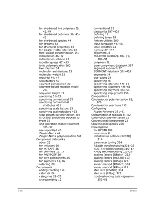
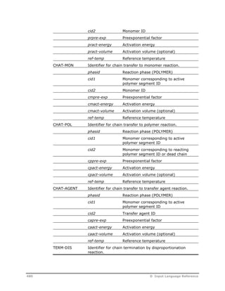
![D Input Language Reference
This section describes the input language for:
Specifying Components, 447
Specifying Component Attributes, 451
Specifying Attribute Scaling Factors, 453
Requesting Distribution Calculations, 454
Calculating End Use Properties, 454
Specifying Physical Property Inputs, 456
Specifying Step-Growth Polymerization Kinetics, 460
Specifying Free-Radical Polymerization Kinetics, 467
Specifying Emulsion Polymerization Kinetics, 477
Specifying Ziegler-Natta Polymerization Kinetics, 484
Specifying Ionic Polymerization Kinetics, 494
Specifying Segment-Based Polymer Modification Reactions, 501
Specifying Components
This section describes the input language for specifying components.
Naming Components
Following is the input language used to name components.
Input Language for Components
COMPONENTS cid [cname] [outid] / ...
Input Language Description for Components
COMPONENTS cid Component ID. Used to refer to the component in
all subsequent input and is also used to identify the
component in the simulation report. Aspen Plus
input language conventions and naming guidelines
apply to this keyword.
D Input Language Reference 447](https://image.slidesharecdn.com/aspenpolymersunitopsv82-usr-141128134016-conversion-gate02/85/Aspen-polymersunitopsv8-2-usr-459-320.jpg)


![userpropid User property set ID. This property must be different from
built-in properties. (See Aspen Physical Property System
Physical Property Data documentation.)
SUBROUTINE Name of user-supplied subroutine for calculating the
property. For details on writing the user-supplied subroutine,
see Aspen Plus User Models reference manual.
FLASH FLASH=NO Does not flash the stream before the
user-supplied subroutine is called
(Default)
FLASH=
NOCOMPOSITE
Does not flash the stream for total
stream properties (When PHASE=T in the
Prop-Set paragraph), but flashes for any
other phase specification
FLASH=YES Always flashes stream before the user-supplied
subroutine is called
UNIT-TYPE Units keyword for the property. If not entered, unit
conversion is not performed on property values returned from
the user-supplied subroutine.
UNIT-LABEL Unit label for the property printed in the report. A unit label is
used only when unit conversion is performed by the user-supplied
subroutine (that is, when UNIT-TYPE is not given).
COMP-DEP COMP-DEP=YES Property is component property
COMP-DEP=NO Property is a mixture property (Default)
Specifying Physical Property
Inputs
This section describes the input language for specifying physical property
inputs. More information on physical property methods and models is given in
Volume 2 of this User Guide.
Specifying Property Methods
Following is the input language used to specify property methods.
Input Language for Property Methods
PROPERTIES opsetname keyword=value /
opsetname [sectionid-list] keyword=value /...
Optional keywords:
FREE-WATER SOLU-WATER HENRY-COMPS
HENRY-COMPS henryid cid-list
456 D Input Language Reference](https://image.slidesharecdn.com/aspenpolymersunitopsv82-usr-141128134016-conversion-gate02/85/Aspen-polymersunitopsv8-2-usr-468-320.jpg)
![HENRY-COMPS HC INI1
PROPERTIES POLYNRTL HENRY-COMPS=HC
Specifying Property Data
Following is the input language used to specify property data.
Input Language for Property Data
PROP-DATA
PROP-LIST paramname [setno] / . . .
PVAL cid value-list / value-list / . . .
PROP-LIST paramname [setno] / . . .
BPVAL cid1 cid2 value-list / value-list / . . .
COMP-LIST cid-list
CVAL paramname setno 1 value-list
COMP-LIST cid2-list
BCVAL paramname setno 1 cid1 value-list /
1 cid1 value-list / . . .
Physical property models require data in order to calculate property values.
Once you have selected the property method(s) to be used in your simulation,
you must determine the parameter requirements for the models contained in
the property method(s), and ensure that they are available in the databanks.
If the model parameters are not available from the databanks, you may
estimate them using the Property Constant Estimation System, or enter them
using the PROP-DATA or TAB-POLY paragraphs. The input language for the
PROP-DATA paragraphs is as follows. Note that only the general structure is
given, for information on the format for the input parameters required by
polymer specific models see the relevant chapter in Volume 2 of this User
Guide.
Input Language Description for Property Data
PROP-LIST Used to enter parameter names and data set numbers.
PVAL Used to enter the PROP-LIST parameter values.
BPVAL Used to enter the PROP-LIST binary parameter values.
COMP-LIST Used to enter component IDs.
CVAL Used to enter the COMP-LIST parameter values.
BCVAL Used to enter the COMP-LIST binary parameter values.
paramname Parameter name
458 D Input Language Reference](https://image.slidesharecdn.com/aspenpolymersunitopsv82-usr-141128134016-conversion-gate02/85/Aspen-polymersunitopsv8-2-usr-470-320.jpg)
![Input Language for Property Parameter Estimation
ESTIMATE [option]
STRUCTURES
method SEG-id groupno nooccur / groupno nooccur /...
Input Language Description for Property Parameter Estimation
The main keywords for specifying property parameter estimation inputs are
the ESTIMATE and the STRUCTURES paragraphs. A brief description of the
input language for these paragraphs follows. For more detailed information
please refer to the Aspen Physical Property System Physical Property Data
documentation.
option Option=ALL Estimate all missing parameters (default)
method Polymer property estimation method name
SEG-id Segment ID defined in the component list
groupno Functional group number (group IDs listed in Appendix B of
Volume 2 of this User Guide)
nooccur Number of occurrences of the group
Input Language Example for Property Parameter Estimation
ESTIMATE ALL
STRUCTURES
VANKREV ABSEG 115 1 ;-(C6H4)-
VANKREV BSEG 151 2 / 100 2 ; -COO-CH2-CH2-COO-VANKREV
ABSEG 115 1 / 151 2 / 100 2 ;-(C6H4)-COO-CH2-CH2-COO-Specifying
Step-Growth
Polymerization Kinetics
Following is the input language for the STEP-GROWTH REACTIONS paragraph.
Input Language for Step-Growth Polymerization
REACTIONS rxnid STEP-GROWTH
DESCRIPTION '...'
REPORT REPORT=yes/no RXN-SUMMARY=yes/no RXN-DETAILS=yes/noI
STOIC reactionno compid coeff / ...
RATE-CON setno pre-exp act-energy [T-exp] [T-ref] [USER-RC=number]
[CATALYST=compid] [CAT-ORDER=value]
POWLAW-EXP reactionno compid exponent /
[ASSIGN reactionno [ACTIVITY=value] RC-SETS=setno-list]
SPECIES POLYMER=polymerid OLIGOMER=oligomer-list
REAC-GRP groupid type /...
SPEC-GROUP compid groupid number / groupid number / ...
460 D Input Language Reference](https://image.slidesharecdn.com/aspenpolymersunitopsv82-usr-141128134016-conversion-gate02/85/Aspen-polymersunitopsv8-2-usr-472-320.jpg)
![RXN-SET rxn-setno
[A-NUCL-SPEC=compid] [A-ELEC-GRP=groupid] &
[V-ELEC-SPEC=compid] [V-NUCL-GRP=groupid] &
[V-NUCL-SPEC=compid] [V-ELEC-GRP=groupid] &
RC-SETS=rc-setno-list
SG-RATE-CON rc-setno
[CAT-SPEC=compid] [CAT-GRP=groupid] &
sgpre-exp [sgact-energy] [sgt-exp] [sgt-ref] [USER-RC=number]
SUBROUTINE KINETICS=kinname RATECON=rcname MASSTRANS=mtname
USER-VECS NINTK=nintk NREALK=nrealk NINTRC=nintrc &
NREALRC=nrealc NINTMT=nintmt NREALMT=nrealmt &
NIWORK=niwork NWORK=nwork NURC=nurc
INTK value-list
REALK value-list
INTRC value-list
REALRC value-list
INTMT value-list
REALMT value-list
INCL-COMPS compid-list
REAC-TYPE FOR-CON=yes/no REV-CON=yes/no REARRANGE=yes/no
EXCHANGE=yes/no
CONVERGENCE SOLVE-ZMOM=yes/no OLIG-TOL=tolerance
OPTIONS REAC-PHASE=phaseid CONC-BASIS=basis SUPPRESS-WARN=yes/no
USE-BULK=yes/no
The keywords for specifying rate constant parameters for the built-in
reactions, and for specifying user reactions are described here.
Input Language Description for Step-Growth Polymerization
rxnid Unique paragraph ID.
DESCRIPTION Up to 64 characters between double quotes.
REPORT Reaction report options- controls writing of reaction report
in .REP file.
REPORT=YES Print reaction report
REPORT=NO Do not print reaction report
RXN-SUMMARY=
YES
Print stoichiometry for each model-generated
and user-specified reaction.
(Default).
RXN-SUMMARY=
NO
Do not print this summary.
RXN-DETAILS=YES Print stoichiometry, rate constants, and
probability factors for each model-generated
and user-specified reaction.
RXN-DETAILS=NO Do not print this detailed summary.
STOIC Used to specify stoichiometry for user reactions.
Reactionno Reaction number
compid Component ID
D Input Language Reference 461](https://image.slidesharecdn.com/aspenpolymersunitopsv82-usr-141128134016-conversion-gate02/85/Aspen-polymersunitopsv8-2-usr-473-320.jpg)


![Input Language for Free-Radical Polymerization
REACTIONS reacid FREE-RAD
PARAM QSSA=yes/no QSSAZ=yes/no QSSAF=yes/no RAD-INTENS=value
SPECIES POLYMER=cid INITIATOR=cid-list MONOMER=cid-list INHIBITOR=cid-list &
SOLVENT=cid-list BI-INITIATOR=cid-list COINITIATOR=cid-list CHAINTAG=cid-list &
CATALYST=cid-list INIT-DEC cid idpre-exp idact-energy idact-volume ideffic &
idnrad ref-temp [GEL-EFFECT=gelid] [EFF-GEFF=gelid] [COEF1=value BYPROD1=cid] &
[COEF2=value BYPROD2=cid]
INIT-CAT cid1 cid2 icpre-exp icact-energy icact-volume iceffic
icnrad ref-temp [GEL-EFFECT=gelid] [EFF-GEFF=gelid] &
[COEF1=value BYPROD1=cid] [COEF2=value BYPROD2=cid]
INIT-SP cid1 cid2 ispre-exp isact-energy isact-volume ref-temp &
[GEL-EFFECT=gelid] [COEF1=value BYPROD1=cid] [COEF2=value BYPROD2=cid]
INIT-SP-EFF cid coeffa coeffb coeffc
BI-INIT-DEC cid bdpre-exp bdact-energy bdact-volume bdeffic
ref-temp [GEL-EFFECT=gelid] [EFF-GEFF=gelid] &
[COEF1=value BYPROD1=cid] [COEF2=value BYPROD2=cid]
SEC-INIT-DEC cid sdpre-exp sdact-energy sdact-volume sdeffic
ref-temp [GEL-EFFECT=gelid] [EFF-GEFF=gelid] &
[COEF1=value BYPROD1=cid] [COEF2=value BYPROD2=cid]
CHAIN-INI cid cipre-exp ciact-energy ciact-volume ref-temp [GEL-EFFECT=gelid]
PROPAGATION cid1 cid2 prpre-exp pract-energy pract-volume ref-temp [GEL-EFFECT=gelid]
CHAT-MON cid1 cid2 cmpre-exp cmact-energy cmact-volume ref-temp [GEL-EFFECT=gelid]
CHAT-POL cid1 cid2 cppre-exp cpact-energy cpact-volume ref-temp [GEL-EFFECT=gelid]
CHAT-AGENT cid1 cid2 capre-exp caact-energy caact-volume ref-temp [GEL-EFFECT=gelid]
CHAT-SOL cid1 cid2 cspre-exp csact-energy csact-volume ref-temp [GEL-EFFECT=gelid]
B-SCISSION cid bspre-exp bsact-energy bsact-volume ref-temp [GEL-EFFECT=gelid]
TERM-DIS cid1 cid2 tdpre-exp tdact-energy tdact-volume ref-temp [GEL-EFFECT=gelid]
TERM-COMB cid1 cid2 tcpre-exp tcact-energy tcact-volume ref-temp [GEL-EFFECT=gelid]
INHIBITION cid1 cid2 inpre-exp inact-energy inact-volume ref-temp [GEL-EFFECT=gelid]
SC-BRANCH cid1 cid2 scpre-exp scact-energy scact-volume ref-temp [GEL-EFFECT=gelid]
HTH-PROP cid1 cid2 hppre-exp hpact-energy hpact-volume ref-temp [GEL-EFFECT=gelid]
CIS-PROP cid1 cid2 pcpre-exp pcact-energy pcact-volume ref-temp [GEL-EFFECT=gelid]
TRANS-PROP cid1 cid2 ptpre-exp ptact-energy pcact-volume ref-temp [GEL-EFFECT=gelid]
TDB-POLY cid1 cid2 tdpre-exp tdact-energy tdact-volume ref-temp [GEL-EFFECT=gelid]
PDB-POLY cid1 cid2 pbpre-exp pbact-energy pbact-volume ref-temp [GEL-EFFECT=gelid]
GEL-EFFECT gelid CORR-NO=corrno &
MAX-PARAMS=maxparams GE-PARAMS=paramlist / ...
SUBROUTINE GEL-EFFECT=subname
OPTIONS REAC-PHASE=phaseid SUPRESS-WARN=yes/no USE-BULK=yes/no
Input Language Description for Free-Radical Polymerization
reacid Paragraph ID.
PARAM Used to specify polymerization mechanism, radiation
intensity, and request the Quasi-Steady-State
Approximation (QSSA).
RAD-INTENS=
value
Used to specify a value for the radiation
intensity to be used for the induced
initiation reaction (default is 1.0)
QSSA=
YES/NO
Used to request QSSA for all moments
(default is NO)
468 D Input Language Reference](https://image.slidesharecdn.com/aspenpolymersunitopsv82-usr-141128134016-conversion-gate02/85/Aspen-polymersunitopsv8-2-usr-480-320.jpg)


![Input Language for Emulsion Polymerization
REACTIONS reacid EMULSION
PARAM KBASIS=monomer/aqueous
SPLIT-PM spm-cid kll
SPECIES INITIATOR=cid MONOMER=cid INHIBITOR=cid &
DISPERSANT=cid . . .
INIT-DEC phasid cid idpre-exp idact-energy [idact-volume] ideffic &
idnrad ref-temp
INIT-CAT phased cid1 cid2 icpre-exp icact-energy [icact-volume] iceffic &
icnrad ref-temp
INIT-ACT phasid cid1 cid2 iapre-exp iaact-energy [iaact-volume] iaeffic &
ianrad ref-temp
PROPAGATION phasid cid1 cid2 prpre-exp pract-energy [pract-volume] ref-temp
CHAT-MON phasid cid1 cid2 cmpre-exp cmact-energy [cmact-volume] ref-temp
CHAT-POL phasid cid1 cid2 cppre-exp cpact-energy [cpact-volume] ref-temp
CHAT-AGENT phasid cid1 cid2 capre-exp caact-energy [caact-volume] ref-temp
TERM-DIS phasid cid1 cid2 tdpre-exp tdact-energy [tdact-volume] ref-temp
TERM-COMB phasid cid1 cid2 tcpre-exp tcact-energy [tcact-volume] ref-temp
INHIBITION phasid cid1 cid2 inpre-exp inact-energy [inact-volume] ref-temp
REDUCTION phasid cid1 cid2 rdpre-exp rdact-energy [rdact-volume] rdeffic &
rdnrad ref-temp
OXIDATION phasid cid1 cid2 oxpre-exp oxact-energy [oxact-volume] ref-temp
GEL-EFFECT GETYPE=reactiontype CORR-NO=corrno &
MAX-PARAMS=maxparams GE-PARAMS=paramlist / ...
SUBROUTINE GEL-EFFECT=subname
ABS-MIC ampre-exp amact-energy
ABS-PART appre-exp apact-energy
DES-PART dppre-exp dpact-energy
EMUL-PARAMS emulid cmc-conc area
Input Language Description for Emulsion Polymerization
reacid Paragraph ID.
PARAM Use to enter basis parameters.
KBASIS=
monomer/
aqueous
Basis for phase split ratios
SPLIT-PM Used to enter homosaturation solubility of species in the
polymer phase.
spm-cid Component ID of the species
partitioning into the polymer phase
kll Ratio of mass fraction of species in
polymer phase to mass fraction in
reference phase. KBASIS determines
whether the reference phase is the
monomer of aqueous phase
SPECIES Reacting species identification. This sentence is used to
associate components in the simulation with species in the
built-in free-radical kinetic scheme. The following species
keywords are currently valid
INITIATOR CATALYST MONOMER
CHAINTAG DISPERSANT INHIBITOR
POLYMER EMULSIFIER ACTIVATOR
REDOX-AGENT REDUCTANT
478 D Input Language Reference](https://image.slidesharecdn.com/aspenpolymersunitopsv82-usr-141128134016-conversion-gate02/85/Aspen-polymersunitopsv8-2-usr-490-320.jpg)


![OPTIONS Specify reaction model options.
REAC-PHASE=
phaseid
Specify the reacting phase as L, L1, L2, or V
(default is L)
SUPRESS-WARN=
yes/no
YES: do not print warnings when the
specified phase is not present
NO: always print warnings when the
specified phase is not present (default)
USE-BULK=
yes/no
YES: force the model to apply the specified
reaction kinetics to the bulk phase when the
specified phase is not present (default)
NO: rates are set to zero when the specified
phase is not present
Input Language Example for Ionic Polymerization
REACTIONS rxnid SEGMENT-BAS
DESCRIPTION '...'
PARAM TREF=value PHASE=V/L/L1/L2 SOLVE-ZMOM=YES/NO &
[SUPRESS-WARN=yes/no] [USE-BULK=yes/no] CBASIS=basis &
[REAC-SITE=siteno S-BASIS=basis]
SPECIES POLYMER=polymerid
STOIC reactionno compid coef / ...
RATE-CON reactionno pre-exp act-energy [t-exp] [TREF=ref-temp] &
[CATALYST=cid CAT-ORDER=value] [USER-RC=userid] / ...
POWLAW-EXP reactionno compid exponent /
[ASSIGN reactionno [ACTIVITY=value] RC-SETS=setno-list]
SUBROUTINE RATECON=rcname MASSTRANS=mtname
USER-VECS NINTRC=nintrc NREALRC=nrealc NINTMT=nintmt NREALMT=nrealmt &
NIWORKRC=niwork NWORKRC=nwork NIWORKMT=niwork NWORKMT=nwork &
NURC=nurc
INTRC value-list
REALRC value-list
INTMT value-list
REALMT value-list
Specifying Segment-Based
Polymer Modification Reactions
The input language for the SEGMENT-BAS REACTIONS paragraph is described
here.
Input Language for Segment-Based Polymer Modification Reactions
D Input Language Reference 501](https://image.slidesharecdn.com/aspenpolymersunitopsv82-usr-141128134016-conversion-gate02/85/Aspen-polymersunitopsv8-2-usr-513-320.jpg)
![REACTIONS rxnid SEGMENT-BAS
DESCRIPTION '...'
PARAM T-REFERENCE=value PHASE=V/L/L1/L2 CBASIS=basis &
SOLVE-ZMOM=YES/NO SPECIES POLYMER=polymerid
STOIC reactionno compid coef / ...
RATE-CON reactionno pre-exp act-energy [t-exp] / ...
POWLAW-EXP reactionno compid exponent /
The keywords for specifying rate constant parameters, reaction stoichiometry,
and reacting polymer are described here.
Input Language Description for Segment-Based Polymer Modification
Reactions
reacid Unique paragraph ID.
DESCRIPTION Up to 64 characters between double quotes.
PARAM Used to enter reaction specifications.
T-REF=
value
Reference temperature. If no reference
temperature is given, the term 1/Tref is
dropped from the rate expression:
rate C k e j j oi
Ea
i
1 1
ij R T T
ref
For more information, see the Segment-
Based Reaction Model section in Chapter 3.
PHASE=V/L/L1
/L2
Reacting phase
CBASIS Basis for power law rate expression. Choices
are:
MOLARITY
MOLALITY
MOLEFRAC
MASSFRAC
MASSCONC
SUPRESS-WARN=
yes/no
YES: do not print warnings when the
specified phase is not present
NO: always print warnings when the
specified phase is not present (default)
USE-BULK=
yes/no
YES: force the model to apply the specified
reaction kinetics to the bulk phase when the
specified phase is not present (default)
NO: rates are set to zero when the specified
phase is not present
SOLVE-ZMOM=
Option to explicitly solve for zeroth moment
based on segment types (default=no)
502 D Input Language Reference](https://image.slidesharecdn.com/aspenpolymersunitopsv82-usr-141128134016-conversion-gate02/85/Aspen-polymersunitopsv8-2-usr-514-320.jpg)