The document summarizes the results of an exercise on artificial neural networks and deep learning. It covers topics like supervised learning algorithms, recurrent neural networks, deep feature learning, and generative models. For a regression problem, it finds that a neural network with one hidden layer, 20 hidden units, and trained with the Levenberg-Marquardt algorithm achieves the best performance on a test set, with a mean squared error close to zero. Further improvements could involve additional hyperparameter tuning, cross-validation, or adding regularization to improve generalization.

1. Faculty of Engineering Science
MSc in Artificial Intelligence
Option: Engineering and Computer Science
Artificial Neural Networks
& Deep Learning
Exercise Session Report
PART I: Supervised Learning and Generalization
PART II: Recurrent Neural Networks
PART III: Deep Feature Learning
PART IV: Generative Models
Evangelia OIKONOMOU
r0737756@kuleuven.com
Oikonomou.elin@gmail.com
Leuven, August 2019

2. 1
TABLE OF CONTENTS
PART I: SUPERVISED LEARNING AND GENERALIZATION...................................................................................2
1 THE PERCEPTRON ......................................................................................................................................................2
1.1 Function approximation & Learning from noisy data.............................................................................2
1.2 Personal Regression Example........................................................................................................................3
2 BAYESIAN INFERENCE.................................................................................................................................................5
PART II: RECURRENT NEURAL NETWORKS......................................................................................................6
1 HOPFIELD NETWORK..................................................................................................................................................6
2 LONG SHORT-TERM MEMORY NETWORKS.....................................................................................................................7
2.1 Time Series Prediction ...................................................................................................................................7
2.2 Long short-term memory network ................................................................................................................7
PART III: DEEP FEATURE LEARNING..............................................................................................................10
1 PRINCIPAL COMPONENT ANALYSIS .............................................................................................................................10
2 STACKED AUTOENCODERS.........................................................................................................................................11
3 CONVOLUTIONAL NEURAL NETWORKS ........................................................................................................................12
PART IV: GENERATIVE MODELS ...................................................................................................................14
1 RESTRICTED BOLTZMANN MACHINES..........................................................................................................................14
2 DEEP BOLTZMANN MACHINES...................................................................................................................................15
3 GENERATIVE ADVERSARIAL NETWORKS .......................................................................................................................16
4 OPTIMAL TRANSPORT ..............................................................................................................................................17

3. 2
Artificial Neural Networks & Deep Learning
Evangelia OIKONOMOU
MSc. in Artificial Intelligence, August 2019
PART I: Supervised Learning and Generalization
1 The perceptron
1.1 Function approximation & Learning from noisy data
Using the given script, we train a neural network with 1 hidden layer and 50 units, using different training algorithms. We
start by comparing gradient descent with quasi Newton algorithm. Both algorithms produce poor function estimation
when trained for few epochs, like 1 and 15. The neural network is trained for 1000 epochs, the quasi Newton algorithm
returns a good function estimation, in contradiction to gradient descent, whose performance remains poor.
Quasi Newton vs Gradient Descent
When comparing gradient descent with Levenberg-Marquardt algorithm, the difference in performance is even larger, as
the latter produces a good function approximation after only 15 epochs of training and the error gets minimized even
further after more epochs. Gradient descent with adaptive learning rate has improved performance compared to gradient
descent algorithm however the error remains high. Fletcher-Reeves conjugate gradient algorithm and Polak-Ribiere
conjugate gradient algorithm show good performance in estimating the underlying function after 1000 epochs with an
error of 0.09-0.10%. Overall, the Levenberg-Marquardt algorithm is the option with the best performance in the noiseless
case.

4. 3
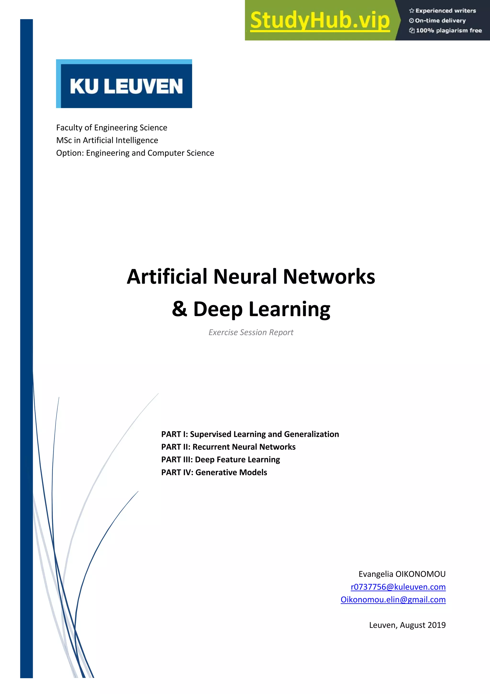
Levenberg-Marquardt vs GD GD with adaptive learning rate vs GD Fletcher-Reeves vs Polak-Ribiere
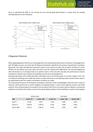
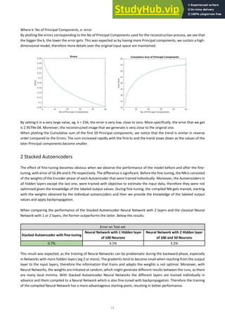
We proceed by adding noise to the data, training the models using different training algorithms like previously and by
calculating the mean squared error of the estimated outputs compared to the noiseless y values. In this case, the Fletcher-
Reeves, Polak-Ribiere and Levenberg-Marquardt algorithm after only 15 epochs approximate the underlying function
with the smallest training error, despite the noise in the data. Overall, the MSE are higher when there is noise in the data.
Without Noise With Noise 0.1*randn(1,length(y))
MSE Epoch 1 Epochs 15 Epochs 1000 Epoch 1 Epochs 15 Epochs 1000
GD 368.84% 185.40% 32.75% 572.02% 299.55% 21.27%
GD w Adaptive Learning 269.16% 176.25% 11.12% 601.91% 169.35% 11.67%
Fletcher-Reeves 206.56% 23.97% 0.09% 372.37% 19.77% 0.56%
Polak-Ribiere 237.89% 19.13% 0.10% 249.84% 41.75% 0.59%
quasi Newton 156.63% 11.30% 0.03% 314.56% 8.22% 0.70%
Levenberg-Marquardt 11.59% 0.01% 1.90E-09 12.85% 0.59% 0.71%
All the models get trained within a few seconds, with the longest being the training with 1000 epochs which lasts 3sec.
The basic gradient descent algorithm yields low performance, as the direction of the weights while training is not always
the direction of the local minima and the learning rate is an arbitrary fixed value. Those issues are tackled with Newton
method, where we consider the second order Taylor expansion in a point x* where gradient is zero. By analysing the
equations, we get w* = w - H-1
g, therefore the optimal weight vector w* is an update of the current weights w moving
towards a direction of gradient g, using a learning parameters H-1
, the inverse of the Hessian. Levenberg-Marquardt is
based on Newton method and it imposes the extra constraint of the step size ||Δx||2 = 1, therefore we consider the
Lagrangian. From the optimality conditions we obtain Δx = -[H + λΙ]-1
g. The term λΙ is a positive definite matrix that is
added to the Hessian in order to avoid ill-conditioning.
1.2 Personal Regression Example
In order to create the independent samples for the training and evaluation of Neural Networks, we merge all the data
(X1, X2, Tnew) into one matrix p with 3 rows and 13600 columns, in which the rows correspond to the two input variables
and the Target data. Afterwards, using the datasample command, we create 3 subsets out of p, with 3 rows and 1000
columns each. For training the model, we will use the first 2 rows as input variables and the last row as target data. In
order to visualize the training set, we create a 3D scatter plot with dimensions X1, X2 and Tnew.

5. 4
It is important to include during the training process the validation set, as it prevents overfitting of the model over the
training set during the training. The model gets optimized on the performance on the validation set rather than on the
training set. The test set is used in order to evaluate the performance of the model in unseen data, ensuring good
generalization.
In order to define a suitable model for our problem, we will train the Neural Network, using the training and validation
set, different training algorithms, No of hidden layers (1 and 2) and No of hidden units per layer (2,5,10 or 20). Finally,
we calculate the mean squared error of the estimated T and the actual T value of the test set.
Initially, we start the training with models of 1 hidden layer. We see that the best performance over the test set (MSE
close to zero) occurs from the Levenberg-Marquardt with 20 hidden units. By plotting the overall results, we see an
improvement on the performance as we increase the number of hidden units in most of the functions, with some
exceptions. When we train the neural networks with 2 hidden layers, we notice that the performance in most cases
improves when comparing models with the same number of hidden units per layer. The Levenberg-Marquardt algorithm
with 10 hidden units per layer produces the smallest error of the test set.
NN with 1
Hidden Layer
GD
GD w Adaptive
Learning rate
Fletcher-
Reeves
Polak-Ribiere Quasi Newton
Levenberg-
Marquardt
numN = 5 12.23% 9.46% 13.29% 4.67% 2.33% 3.01%
numN = 10 8.07% 5.80% 7.95% 13.68% 3.14% 3.09%
numN = 20 9.53% 4.30% 7.91% 1.42% 1.50% 2.87e-05
NN with 2
Hidden Layers
GD
GD w Adaptive
Learning rate
Fletcher-
Reeves
Polak-Ribiere Quasi Newton
Levenberg-
Marquardt
NumN = 2 16.13% 12.98% 15.87% 6.94% 5.54% 5.34%
NumN = 5 13.94% 7.00% 8.45% 5.16% 3.10% 1.66%
NumN = 10 5.18% 5.09% 14.81% 1.20% 1.00% 0.27%
Judging from the above results, we will choose the Levenberg-Marquardt algorithm with 1 hidden layer and 20 hidden
units. In order to improve the performance further, we could run further combinations of no of hidden units and hidden
layers for the specific algorithm and perform Parameter Tuning mechanics or 10-fold Cross Validation. Another method
to ensure good generalization of the model is to introduce a regularization term in the objective function, which
minimizes the squared weights in order to avoid overfitting. By monitoring regularization, there is a balance between a

6. 5
focus on optimizing the MSE on the training set and ensuring good generalization in unseen data, by avoiding
overdependencies on the training set.
Neural Network with 1 Hidden Layer Neural Network with 2 Hidden Layers
2 Bayesian Inference
When applying Bayesian Inference as training algorithm and comparing the performance of previous training algorithms
with 50 hidden neurons, we notice that the Bayesian framework outperforms the previous top-performer Levenberg-
Marquardt. The model with Bayesian framework results to very small errors after only 15 epochs, therefore it is more
efficient. On the without noise case, when we tried to train the network with 1000 epochs, the training stopped only
after 162 iterations as it converges faster to an optimal minima. In the case with noisy data, the performance is inferior
compared to noiseless case, however still outperforms all the rest training algorithms.
Overparameterization of the model with 100 or 200 hidden units is not recommended, as it results in higher errors. This
is an effect of overfitting in the model. We need to consider that there are only 189 input data, therefore there needs to
be a good balance with the number of parameters we add to our model.
The improved performance of the Bayesian Framework compared to other methodologies results from the 3 levels of
inference, which optimize the w vector (weights), the hyperparameters a and b of the objective function and model
selection. Since all those aspects are included in the framework itself, there is no need to split our dataset in training and
validation set, therefore the model can train on the whole dataset, without risk of overfitting or need for early stopping.
Without Noise With Noise
MSE numN = 50 numN = 100 numN = 50 numN = 100 NumN = 200
Epoch 1 13.46% 4.45% 7.44% 4.88% 5.62%
Epochs 15 5.00E-06 2.59E-05 0.53% 0.88% 0.96%
Epochs 1000 6.15E-11 7.26E-12 0.55% 0.92% 0.97%

7. 6
Artificial Neural Networks & Deep Learning
Evangelia OIKONOMOU, r0737756
MSc. in Artificial Intelligence, August 2019
PART II: Recurrent Neural Networks
1 Hopfield Network
We initiate a Hopfield Network with 3 attractors T and start with 25 vectors. We run the model starting with 15 iterations,
however we notice that not all vectors have been reached an attractor. The training is complete when the energy function
which is evolving over time to some lower energy point, stops when it reaches an equilibrium at the moment that all
vectors have reached one of the available attractors. After increasing the number of iterations to 25, all the vectors have
been reached either one of the three initial attractors or a fourth attractor that has been added by the model. These
unwanted attractors are called spurious states and they are linear combinations of the stored patterns.
We execute the rep2 and rep3 scripts and set starting points with high symmetry compared to the stored patterns. In
both cases we notice the phenomenon of spurious states. Moreover we notice the extreme phenomenon of initiating a
point which is symmetrical to the stored patterns and it immediately converts into an attractor itself.

8. 7
2 Long Short-Term Memory Networks
2.1 Time Series Prediction
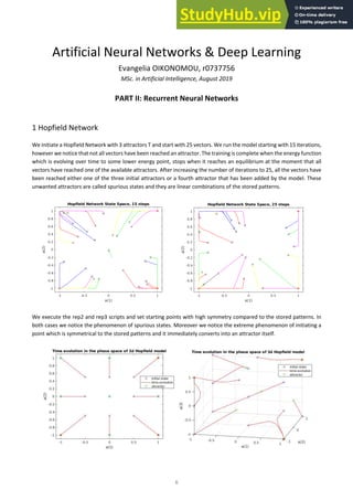
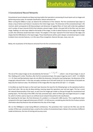
To make a prediction of the next 100 points of the Santa Fe dataset, we start by scaling the train set and the test set by
subtracting the mean of the whole dataset and devising by the standard deviation of the dataset. We use the
getTimeSeriesTrainData command to define the number of lags p, which produces a matrix [p x n] that is used as
training set. The training algorithm that we choose is the Levenberg-Marquardt, as it produced the best results during
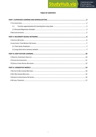
the first exercise session. We train the model for several p values (lag) and number of neurons and calculate the MSE for
each combination. The winning pairs are p = 10 and numN = 5 and 10. We visualize the test target and the prediction and
indeed the results are satisfying.
MSE P = 2 P = 5 P = 10 P = 20 P = 50
numN = 2 22.1% 23.9% 2.1% 49.7% 2.6%
numN = 5 9.0% 8.0% 0.8% 2.4% 40.1%
numN = 10 5.6% 5.7% 0.8% 7.6% 27.1%
numN = 20 4.9% 3.1% 0.9% 2.0% 18.1%
numN = 50 6.4% 4.9% 1.5% 30.4% 44.2%
Santa Fe Time-Series prediction, p = 10, numN = 10
2.2 Long short-term memory network
The advantage of using LSTM over Neural Network is that this framework allows us to retain past information in the
training of the model and use it as “memory” in order to make predictions based on current data and relevant learnings
that were obtained in the past. LSTM is able to select on each state which information to delete from the past, which
information to retain and which to further memorise. This structure effectively tackles the challenge of vanishing gradient
that appears in Neural Networks, where the gradient of past moments becomes very small after a number of iterations,
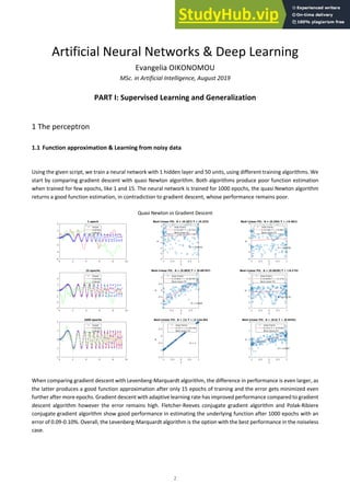
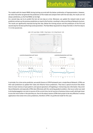
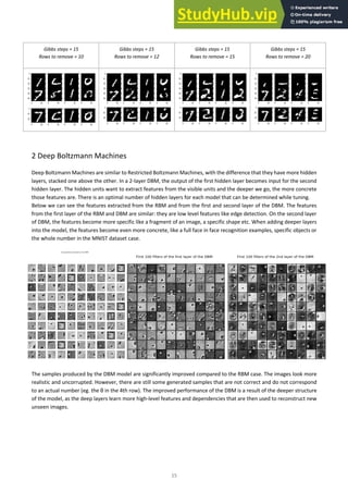
therefore the model is not able to retain the information of the past and inform future predictions. The below diagram
shows the structure of an LSTM model and the operations that take place on a single cell in each iteration.

9. 8
Figure: The LSTM cell structure
Source: https://colah.github.io/posts/2015-08-Understanding-LSTMs/
In order to optimize the model, we test different no of neurons, similar to the Neural Network case, and then try different
combinations of Initial Learn rate and Learn Rate Drop Factor. The Learn Rate controls how much the model changes
after each iteration with respect the loss gradient. A very small learning rate might lead to long training process as it
requires many iterations, while a large value for this hyperparameter might change the W vector to fast in the training
process. The below visualizations explain the impact of learning rate on the gradient descent and convergence of training
process.
Gradient descent with small (top) and large (bottom) learning rates. Effect of various learning rates on convergence (Img Credit: cs231n)
Source: Andrew Ng’s Machine Learning course on Coursera
The other 2 hyperparameters that we tune are the Learn Drop Factor and Learn Drop Period. For instance, a drop factor
of 0.2 and Learn drop Period of 125, it means that the learning rate gets reduced with a factor of 0.2 every 125 iterations.
We train the model, using different values of hyperparameters.
numNlist = [5, 10, 20, 50];
LearnRateList = [0.001, 0.005, 0.01, 0.05, 0.1];
DropFactorList = [0.1, 0.2, 0.5];
DropPeriodList = [25, 50, 125];
Below the learnings from training:
- Small Learn Rates perform better compared to larger values, therefore 0.005 would be our best options. Large
values eg. 0.05 or 0.1 result in large errors as the weights are changing too rapidly in each iteration, therefore
they are not considered in practice.
- Having a small drop period, i.e reducing the learning rate after 25 or 50 iterations, leads to fast decreasing of the
learn rate, therefore the error does not change for the largest part of the training. We set the Drop Period to
125.
- A drop factor of 0.1 reduces the learning rate to 10% of the initial one, while a drop factor of 0.5 only halves it.
We notice during training, that a small drop factor of 0.1 or 0.2, especially when initial learning rate is already
small, results to inefficient training as there is only minimal improvement of the training error.

10. 9
The models with the lowest RMSE during training occurred with the below combination of hyperparameters. However,
we notice that when we generate the predictions of the model and compare them with the test data, the results are not
always satisfactory, as the final RMSE can be high.
As a second step, we try to predict the test set one step at a time. Moreover, we update the network state at each
prediction and we use the previous predictions as input to the function, resulting in a Recurrent Neural Network structure.
The results are significantly improved during that step. Below the training process and the predictions of the first and
second step for the best performing tuned parameters. The Root Mean Squared Error drops from 60.2 in the first step to
7.1 in the second one.
noN = 20 | Learn Rate = 0.005 | Drop Factor = 0.2 | Drop Period = 125
predictAndUpdateState with Ypred predictAndUpdateState with Xtest
In principle, for a time series prediction, we would choose an LSTM framework over a simple Neural Network. LSTMs use
their own predictions to update their state and influence future predictions. They have a special structure that allows
them to have memory of past patterns and special operations of forgetting or memorizing new information. Recurrent
Neural Networks and especially LSTMs deal effectively with the vanishing gradient problem, that occurs when we need
to do backpropagation not only to neurons of the current time, but all neurons of previous times as well, which get closer
to zero the more further in the past they are. Due to the above reasons LSTMs have proven to be very effective in various
applications that evolve time series predictions, therefore LSTM is my preferred model for this case.

11. 10
Deep Learning & Artificial Neural Networks
Evangelia OIKONOMOU, r0737756
MSc. in Artificial Intelligence, August 2019
PART III: Deep Feature Learning
1 Principal Component Analysis
We import the dataset and calculate the mean which is equal to 0.2313. We want to transform the data set into 0 mean
and variance 1, therefore we apply the below transformation:
| xzm = (x - mean(x(:)))/std(x(:)); % convert to 0 mean and 1 variance
When we recalculate the mean on xzm, that is a very small value, close to 0.
Afterwards, we calculate the covariance matrix and its eigenvalues and eigenvectors. From the plot of the diagonal of the
eigenvalues, we see that the majority of eigenvalues have a very small value, close to 0. Only a very few eigenvalues have
a larger value that grows exponentially. The largest eigenvalues in decreasing order are 21.94, 6.11, 2.76, 2.57, 1.77, 1.58
etc. This means that by reducing the dimensionality as low as 1D or 2D, we will still generate good results.
Below the original image of a 3 and the reconstruction images after we applied dimensionality reduction. The more
dimensions we use in order to reconstruct the initial dataset, the more details are preserved in the image and the smaller
the error we get.
Original Image k = 1, e = 27.6% k = 4, e = 22,7%

12. 11
Where k: No of Principal Components, e: error
By plotting the errors corresponding to the No of Principal Components used for the reconstruction process, we see that
the bigger the k, the lower the error gets. This was expected as by having more Principal components, we sustain a high-
dimensional model, therefore more details over the original input space are maintained.
By setting k in a very large value, eg. k = 256, the error is very low, close to zero. More specifically, the error that we get
is 2.9579e-04. Moreover, the reconstructed image that we generate is very close to the original one.
When plotting the Cumulative sum of the first 50 Principal components, we notice that the trend is similar in reverse
order compared to the Errors. The sum increased rapidly with the first ks and the trend slows down as the values of the
later Principal components become smaller.
2 Stacked Autoencoders
The effect of fine-tuning becomes obvious when we observe the performance of the model before and after the fine-
tuning, with error of 16.8% and 0.7% respectively. The difference is significant. Before the fine-tuning, the NN is consisted
of the weights of the Encoder phase of each Autoencoder that were trained individually. Moreover, the Autoencoders in
all hidden layers except the last one, were trained with objective to estimate the Input data, therefore they were not
optimized given the knowledge of the labeled output values. During fine-tuning, the compiled NN gets trained, starting
with the weights obtained by the individual autoencoders and then we provide the knowledge of the labeled output
values and apply backpropagation.
When comparing the performance of the Stacked Autoencoder Neural Network with 2 layers and the classical Neural
Network with 1 or 2 layers, the former outperforms the latter. Below the results:
Error on Test set
Stacked Autoencoder with fine-tuning
Neural Network with 1 Hidden layer
of 100 Neurons
Neural Network with 2 Hidden layer
of 100 and 50 Neurons
0.7% 4.5% 3.2%
This result was expected, as the training of Neural Networks can be problematic during the backward phase, especially
in Networks with more hidden layers (eg 2 or more). The gradients tend to become small when reaching from the output
layer to the input layers, therefore the information that trains and adapts the weights is not optimal. Moreover, with
Neural Networks, the weights are initiated at random, which might generate different results between the runs, as there
are many local minima. With Stacked Autoencoder Neural Networks the different layers are trained individually in
advance and them compiled to a Neural Network which is also fine-tuned with backpropagation. Therefore the training
of the compiled Neural Network has a more advantageous starting point, resulting in better performance.

13. 12
3 Convolutional Neural Networks
Convolutional neural networks are Deep Learning models that specialize in processing of visual inputs such as images and
performing various tasks, for example classification, feature extraction etc.
When running the CNNex.m script, we observe the architecture of the network. The first convolutional layer (layer 2)
shows a map of where each feature is located on the initial image inputs. The dimension of the convolutional layer is 96
11x11x3, which corresponds to 96 features/layers and dimension of applied filters of 11x11 with stride 4x4, padding 0
and 3 number of input channels (R B G) that indicates colored images. Stride is the pixel shift of the filter over the input
image. Padding is an extra layer added on the border of the image, in order to detect features are the edges of the image
as well, that otherwise would have been missed. The weights in this layer represent first level features like edges and
shapes that the CNN detects in the input images. Those initial features will be used in deeper convolutional layers in order
to detect more concrete features, i.e in the case of face recognition, features like eyes, noses, ears, etc.
Below, the visualization of the features extracted from the first convolutional layer.
The size of the output image can be calculated by the formula , where I: size of input image, K: size of
filer, Padding and S: stride. Therefore, after the first convolutional layer, the output image has size O = ((227 - 11 +2X0)/4)
+ 1 = 55. ReLU and Normalization layers do not affect the dimension. During the max Pooling layer, the dimension of the
image gets reduced further. In this step, we apply a window size of 3x3 with stride 2x2. For each window of 3x3 pixels we
keep only the maximum value. The dimension of the image after this step will be (55-3)/2 + 1 = 27 pixels.
In ConvNets we stack the layers so that each layer becomes the input for the following layer so the operations build on
top of each other. We can also do deep stacking, meaning repeat the operations over and over again. This has a result
the reduced dimensionality of the input, as each time the images get smaller as they go through the convolutional and
pooling layers. The final step of the CNN is the fully connected layer, where all filters get rearranged and put in a single
list, which is further used as input to an artificial neural network that performs the classification.
By inspecting the last layer, the final dimension of a problem is a string with 1.000 neurons. This is significantly lower
compared to the input image with dimensions 227x227 = 51.529 neurons, considering also that this list of values contains
information about key features that will determine the class of the image.
We run the CNNDigits.m script trying different architectures. The parameters that I tuned are the filter size and the
number of filters per convolutional layer, as well as the number of convolutional layers. Below is the overview of different
model architectures, the time of training and accuracy score.

14. 13
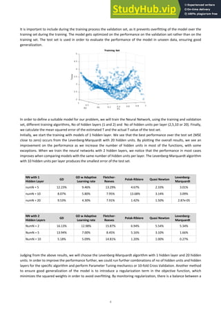
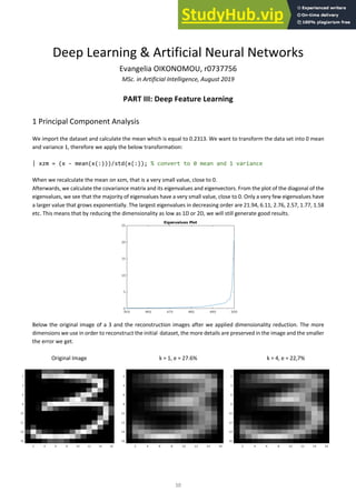
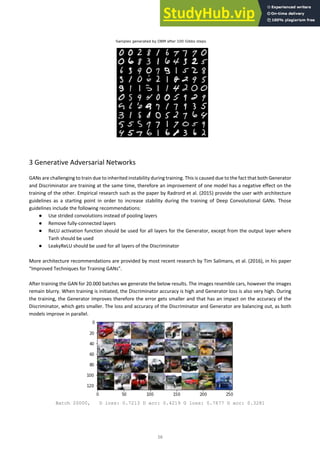
Model 1 2 3 4
Architecture layers = [imageInputLayer([28 28 1])
convolution2dLayer(5,12)
reluLayer
maxPooling2dLayer(2,'Stride',2)
convolution2dLayer(5,24)
reluLayer
fullyConnectedLayer(10)
softmaxLayer
classificationLayer()];
layers = [imageInputLayer([28 28 1])
convolution2dLayer(3,12)
reluLayer
maxPooling2dLayer(2,'Stride',2)
convolution2dLayer(3,24)
reluLayer
fullyConnectedLayer(10)
softmaxLayer
classificationLayer()];
layers = [imageInputLayer([28 28 1])
convolution2dLayer(3,16)
reluLayer
maxPooling2dLayer(2,'Stride',2)
convolution2dLayer(3,32)
reluLayer
fullyConnectedLayer(10)
softmaxLayer
classificationLayer()];
layers = [imageInputLayer([28 28 1])
convolution2dLayer(3,16)
reluLayer
maxPooling2dLayer(2,'Stride',2)
convolution2dLayer(3,32)
reluLayer
convolution2dLayer(3,48)
fullyConnectedLayer(10)
softmaxLayer
classificationLayer()];
Training
Accuracy
Training Time 48,15 sec 40,39 sec 44,18 sec 62,54 sec
Accuracy 0,8344 0,9092 0,9488 0,9668
The model increases in accuracy, when the filter size gets smaller in convolution layer, from 5x5 to 3x3. Further
improvements occur by increasing the No of filters and by adding a third Convolutional layer. Applying those changes,
the accuracy increases by 13,3 percentage points, from 83,4% to 96,7%, while the mini batch accuracy in the final epochs
reaches 100%.

15. 14
Deep Learning & Artificial Neural Networks
Evangelia OIKONOMOU, r0737756
MSc. in Artificial Intelligence, August 2019
PART IV: Generative Models
1 Restricted Boltzmann Machines
For RBMs training, it is not tractable to use Max Likelihood, therefore we solve with Contrastive Divergence (CD) [Hinton,
2002] algorithm. To perform sampling we use Gibbs sampler, with T steps, where T=1 often in practice.
To optimize the model we tune the No of components, No of iterations and Learning Rate. No of components correspond
to No of binary hidden units. The model performs better when increasing the number of hidden units as it learns more
patterns from the training set, however the training time is longer. To avoid long training time, we reduce the no of
iterations. The learning rate controls how much the weights change after each iteration. A large learning rate results in
faster learning, with the downside that it might converge to a sub-optimal set of weights. A small learning rate allows the
model to learn a more optimal or even global-optimal set of weights, however the training takes longer as many iterations
are required. In order to define a combination of hyperparameters for optimal performance, we can either manually try
different combinations or we can perform Parameter Tuning with GridSearchCV.
Below the sampling images generated by the model with No of components = 100, Learning Rate = 0,05, No of Iterations
= 30 and Gibbs steps = 1, compared to the real images. The model produces realistic images which are close to the original
input.
Sampling Images
Real Images
For the reconstruction of unseen images, 1 Gibbs step is not enough to get a good reconstruction, therefore we increase
this hyperparameter to 10 or 15. The reconstructed images are not perfect, on the contrary they are corrupted. The
reconstructions become unreadable after we remove 20 rows.

16. 15
Gibbs steps = 15
Rows to remove = 10
Gibbs steps = 15
Rows to remove = 12
Gibbs steps = 15
Rows to remove = 15
Gibbs steps = 15
Rows to remove = 20
2 Deep Boltzmann Machines
Deep Boltzmann Machines are similar to Restricted Boltzmann Machines, with the difference that they have more hidden
layers, stacked one above the other. In a 2-layer DBM, the output of the first hidden layer becomes input for the second
hidden layer. The hidden units want to extract features from the visible units and the deeper we go, the more concrete
those features are. There is an optimal number of hidden layers for each model that can be determined while tuning.
Below we can see the features extracted from the RBM and from the first and second layer of the DBM. The features
from the first layer of the RBM and DBM are similar: they are low level features like edge detection. On the second layer
of DBM, the features become more specific like a fragment of an image, a specific shape etc. When adding deeper layers
into the model, the features become even more concrete, like a full face in face recognition examples, specific objects or
the whole number in the MNIST dataset case.
The samples produced by the DBM model are significantly improved compared to the RBM case. The images look more
realistic and uncorrupted. However, there are still some generated samples that are not correct and do not correspond
to an actual number (eg. the θ in the 4th row). The improved performance of the DBM is a result of the deeper structure
of the model, as the deep layers learn more high-level features and dependencies that are then used to reconstruct new
unseen images.

17. 16
3 Generative Adversarial Networks
GANs are challenging to train due to inherited instability during training. This is caused due to the fact that both Generator
and Discriminator are training at the same time, therefore an improvement of one model has a negative effect on the
training of the other. Empirical research such as the paper by Radrord et al. (2015) provide the user with architecture
guidelines as a starting point in order to increase stability during the training of Deep Convolutional GANs. Those
guidelines include the following recommendations:
● Use strided convolutions instead of pooling layers
● Remove fully-connected layers
● ReLU activation function should be used for all layers for the Generator, except from the output layer where
Tanh should be used
● LeakyReLU should be used for all layers of the Discriminator
More architecture recommendations are provided by most recent research by Tim Salimans, et al. (2016), in his paper
“Improved Techniques for Training GANs”.
After training the GAN for 20.000 batches we generate the below results. The images resemble cars, however the images
remain blurry. When training is initiated, the Discriminator accuracy is high and Generator loss is also very high. During
the training, the Generator improves therefore the error gets smaller and that has an impact on the accuracy of the
Discriminator, which gets smaller. The loss and accuracy of the Discriminator and Generator are balancing out, as both
models improve in parallel.
Batch 20000, D loss: 0.7213 D acc: 0.4219 G loss: 0.7677 G acc: 0.3281

18. 17
4 Optimal Transport
The Optimal Transport is a popular mathematical framework used to minimize the distance between two marginal
distributions p and q, where p corresponds to the model distribution pθ, and q corresponds to data distribution. This is
solved by considering the Wasserstein Distance between the two marginal distribution, which equals to minimization of
expected value of the probability distribution π over the distances x and x’. It can be expressed as Linear Optimization
problem with contraints, solved by taking the Lagrangian. It solves a common challenge called the assignment problem,
when a quantity of goods represented by marginal probability distributions has to be transported from one place to
another, by minimizing the cost and taking into account the quantities required by the receiving part. W(p, q) = minπ∈Π(p,q)
Eπd(x, x′), with d(x, x′) a distance metric.
In the given script, OT is used in order to transfer the colors between two images. The chosen images show the same
landscape during different times of the day. By executing the code, the color pallet from the first image is transported to
the second image and vice versa.
Optimal Transport has been applied to GANs, making use of the Wasserstein distance between the distributions of the
Generator and Discriminator. The so-called WGAN is more stable during learning compared regular GANs, as we omit the
sigmoid function in front of the function D, therefore its output is real values instead of probabilities between [0,1]. Due
to the zero-sum game, the sum of the Cost function for the discriminator D and generator G is equal to zero.
W(D)
(D,G) = Ex∼pdata[D(x)] − Ez∼pz[D(G(z))]
W(G)
(D, G) = −W(D)
(D, G)
Below we train a standard GAN and a Wasserstein GAN. Both methods produce bad results due to the simple fully-
connected architecture for training efficiency. The Wasserstein GAN tackles better the noise compared to the standard
GAN.
Standard GAN Wasserstein GAN