Download to read offline


![Fundamental Concepts and Definitions ____________________________________________ 39
1.14 Write Boyle’s law and Charle's law.
1.15 Determine the absolute pressure of gas in a tank if the pressure gauge mounted on tank reads 120 kPa
pressure. [221.3 kPa]
1.16 What shall be the volume of a fluid having its specific gravity as 0.0006 and mass as 10 kg?
[16.67 m3
]
1.17 Determine the pressure of compressed air in an air vessel, if the manometer mounted on it shows a
pressure of 3 m of mercury. Assume density of mercury to be 13.6 × 10³ kg/m3 and atmospheric
pressure as 101 kPa. [501.25 kPa]
1.18 Calculate the kinetic energy of a satellite revolving around the earth with a speed of 1 km/s. Assume
acceleration due to gravity as 9.91 m/s2 and gravitational force of 5 kN. [254.8 MJ]
1.19 If the gauge pressure of oil in a tube is 6.275 kPa and oil’s specific gravity is 0.8, then determine depth
of oil inside tube. [80 cm]
1.20 Determine the work required for displacing a block by 50 m and a force of 5 kN. [250 kJ]
1.21 Determine the barometer reading in millimetres of Hg if the vacuum measured on a condenser is 74.5
cm of Hg and absolute pressure is 2.262 kPa. [760mm]
1.22 Determine the absolute pressures for the following;
(i) Gauge pressure of 1.4 MPa
(ii) Vacuum pressure of 94.7 kPa
Take barometric pressure as 77.2 cm of Hg and density of mercury as 13.6 × 10³ kg/m3.
[1.5 MPa, 8.3 kPa]
1.23 Determine the pressure acting upon surface of a vessel at 200 m deep from surface of sea. Take
barometric pressure as 101 kPa and specific gravity of sea water as 1.025. [2.11 MPa]
1.24 A vacuum gauge gives pressure in a vessel as 0.1 bar, vacuum. Find absolute pressure within vessel
in bars. Take atmospheric pressure as 76 cm of mercury column, g = 9.8 m/s2
, density of mercury
= 13.6 g/cm3. [0.91 bar]
1.25 Determine the work done upon a spring having spring constant of 50 kN/m. Spring is stretched to 0.1
m from its unstretched length of 0.05 m. [0.0625 kJ]
1.26 Determine the mass of oxygen contained in a tank of 0.042 m3 at 298 K and 1.5 × 10⁷ Pa considering it
as perfect gas. Also determine the mass using compressibility charts. [8.25, 8.84]
1.27 What will be specific volume of water vapour at 1 MPa and 523 K, if it behaves as ideal gas? Also
determine the same considering generalized compressibility chart. [0.241 m3/kg, 0.234 m3/kg]
1.28 Calculate the pressure of CO2 gas at 27ºC and 0.004 m3/kg treating it as ideal gas. Also determine the
pressure using Van der Waals equation of state. [14.17 MPa, 6.9 MPa]
1.29 Determine molecular weight and gas constant for a mixture of gases having 65% N2, 35% CO2 by mole.
[33.6 kg/k mol. 0.247 kJ/kg . K]
1.30 Considering air as a mixture of 78% N2, 22% O2 by volume determine gas constant, molecular weight,
Cp and Cv for air at 25ºC. [0.2879 kJ/kg . K, 28.88 kg/K mol, 1.0106 kJ/kg . K, 0.722 kJ/kg . K]
1.31 What minimum volume of tank shall be required to store 8 kmol and 4 kmol of O2 and CO2 respectively
at 0.2 MPa, 27ºC ? [149.7 m3]
1.32 Two tanks A and B containing O2 and CO2 have volumes of 2 m3 and 4 m3 respectively. Tank A is at 0.6
MPa, 37ºC and tank B is at 0.1 MPa and 17ºC. Two tanks are connected through some pipe so as to
allow for adiabatic mixing of two gases. Determine final pressure and temperature of mixture.
[0.266 MPa, 30.6ºC]
1.33 Determine the molecular weight and gas constant for some gas having CP = 1.968 kJ/kg . K, Cv = 1.507
kJ/kg . K. [18.04 kg/kmol, 0.461 kJ/kg . K]](https://image.slidesharecdn.com/appliedthermodynamics3rdedition-230807154336-69e627e1/85/Applied-Thermodynamics-3rd-Edition-pdf-56-320.jpg)


![82 _________________________________________________________ Applied Thermodynamics
Solution:
Let mass of steam to be supplied per kg of water lifted be ‘m’ kg. Applying law of energy conservation
upon steam injector, for unit mass of water lifted.
Energy with steam entering + Energy with water entering = Energy with mixture leaving + Heat loss
to surroundings.
2
2
(50)
(720 10 4.18)
2
m
+ × ×
+ 1 × [(24.6 × 103 × 4.18) + (9.81 × 2)]
K.E. Enthalpy Enthalpy P.E
= (1 + m)
2
3 (25)
(100 10 4.18)
2
× × +
+ [m × 12 × 103 × 4.18]
Enthalpy K.E Heat loss
m [3010850] + [102847.62] = (1 + m) . (418312.5) + m[50160]
Upon solving, m = 0.124 kg steam/kg of water
Steam supply rate = 0.124 kg/s per kg of water. Ans.
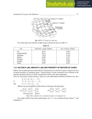
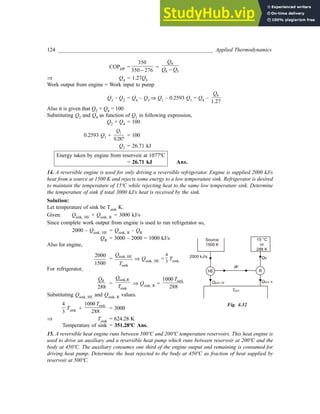
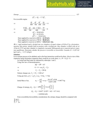
12. An inelastic flexible balloon is inflated from initial empty state to a volume of 0.4 m3 with H2
available from hydrogen cylinder. For atmospheric pressure of 1.0313 bar determine the amount of work
done by balloon upon atmosphere and work done by atmosphere.
Solution:
Balloon after being inflated
Balloon initially empty
Fig. 3.34
Here let us assume that the pressure is always equal to atmospheric pressure as balloon is flexible,
inelastic and unstressed and no work is done for stretching balloon during its filling. Figure 3.34 shows
the boundary of system before and after filling balloon by firm line and dotted line respectively.
Displacement work, W =
cylinder
.
p dV
∫ +
balloon
.
p dV
∫
.
p dV
∫ = 0 as cylinder shall be rigid.
= 0 + p · ∆V
= 0 + 1.013 × 105 × 0.4
= 40.52 kJ
Work done by system upon atmosphere = 40.52 kJ
Work done by atmosphere = – 40.52 kJ Ans.
13. In a steam power plant 5 kW of heat is supplied in boiler and turbine produces 25% of heat added
while 75% of heat added is rejected in condenser. Feed water pump consumes 0.2% of this heat added
](https://image.slidesharecdn.com/appliedthermodynamics3rdedition-230807154336-69e627e1/85/Applied-Thermodynamics-3rd-Edition-pdf-99-320.jpg)


![90 _________________________________________________________ Applied Thermodynamics
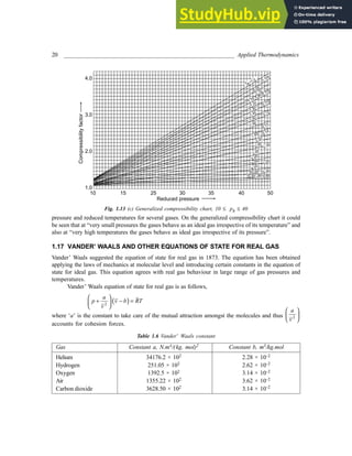
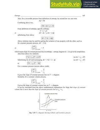
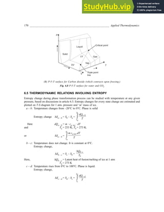
20. An evacuated bottle of 0.5 m3 volume is slowly filled from atmospheric air at 1.0135 bars until the
pressure inside the bottle also becomes 1.0135 bar. Due to heat transfer, the temperature of air inside the
bottle after filling is equal to the atmospheric air temperature. Determine the amount of heat transfer.
[U.P.S.C., 1994]
Solution:
Final system boundary
after filling
Evacuated bottle
Initial system boundary
Valve
Initial system boundary
P = 1.0135 bar
atm
Fig. 3.41
Displacement work; W = 1.0135 × 105 × (0 – 0.5)
W = – 0.50675 × 10⁵ Nm
Heat transfer, Q = 0.50675 × 10⁵ Nm
Heat transfer = 0.50675 × 10⁵ Nm Ans.
21. A compressed air bottle of 0.3 m3 volume contains air at 35 bar, 40°C. This air is used to drive a
turbogenerator sypplying power to a device which consumes 5 W. Calculate the time for which the
device can be operated if the actual output of the turbogenerator is 60% of the maximum theoretical
output. The ambient pressure to which the tank pressure has fallen is 1 bar. For air,
p
C
Cv
= 1.4.
[U.P.S.C. 1993]
Solution:
Here turbogenerator is fed with compressed air from a compressed air bottle. Pressure inside bottle
gradually decreases from 35 bar to 1 bar. Expansion from 35 bar to 1 bar occurs isentropically. Thus,
for the initial and final states of pressure, volume, temperature and mass inside bottle being given as P1,
V1, T1 & m1 and P2, V2, T2 & m2 respectively. It is transient flow process similar to emptying of the
bottle.
1
2
1
P
T
γ
γ
−
=
2
1
T
T , Given: P1 = 35 bar, T1 = 40°C or 313 K
V1 = 0.3 m3; V2 = 0.3 m3
P2 = 1 bar.](https://image.slidesharecdn.com/appliedthermodynamics3rdedition-230807154336-69e627e1/85/Applied-Thermodynamics-3rd-Edition-pdf-107-320.jpg)
![First Law of Thermodynamics _____________________________________________________ 91
T2 = T1
1
2
1
P
T
γ
γ
−
T2 = 113.22 K
By perfect gas law, initial mass in bottle, m1 =
1 1
1
PV
RT =
2
35 10 0.3
0.287 313
× ×
×
m1 = 11.68 kg
Final mass in bottle, m2 =
2 2
2
PV
RT =
2
1 10 0.3
0.287 113.22
× ×
×
m2 = 0.923 kg
Energy available for running turbo generator or work;
W + (m1 – m2) h2 = m1 u1 – m2 u2
W = (m1u1 – m2u2) – (m1 – m2) h2
= (m1 cv T1 – m2 cv T2) – (m1 – m2) · cp · T2
Taking cv = 0.718 kJ/kg . K and cP = 1.005 kJ/kg · K
W = {(11.68 × 0.718 × 313) – (0.923 × 0.718 × 113.22)}
– {(11.68 – 0.923) × 1.005 × 113.22}
W = 1325.86 kJ
This is the maximum work that can be had from the emptying of compressed air bottle between
given pressure limits.
Turbogenerator’s actual output = 5 kJ/s
Input to turbogenerator =
5
0.6
= 8.33 kJ/s.
Time duration for which turbogenerator can be run;
∆t =
1325.86
8.33
∆t = 159.17 sec.
Duration ≈ 160 seconds Ans.
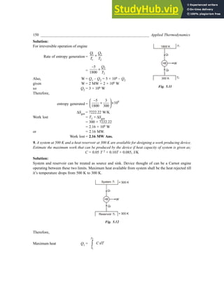
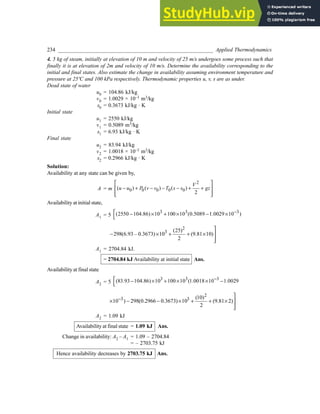
22. 3 kg of air at 1.5 bar pressure and 77°C temperature at state 1 is compressed polytropically to state
2 at pressure 7.5 bar, index of compression being 1.2. It is then cooled at constant temperature to its
original state 1. Find the net work done and heat transferred. [U.P.S.C. 1992]
Solution:
Different states as described in the problem are denoted as 1, 2 and 3 and shown on p-V diagram.
Process 1-2 is polytropic process with index 1.2
So,
2
1
T
T =
1
2
1
n
n
P
P
−
or, T2 = T1
1
2
1
n
n
P
P
−
](https://image.slidesharecdn.com/appliedthermodynamics3rdedition-230807154336-69e627e1/85/Applied-Thermodynamics-3rd-Edition-pdf-108-320.jpg)

![First Law of Thermodynamics _____________________________________________________ 93
Work during process 2-3,
W2–3 = P2 (V3 – V2)
= 7.5 × 10⁵ (0.402 – 0.526)
= – 93 kJ
Work during process 3-1,
W3–1 = P3V3 ln
1
3
V
V
= 7.5 × 105 × 0.402 × ln
2.01
0.402
W3–1 = 485.25 kJ
Net work, Wnet = W1–2 + W2–3 + W3–1
= – 463.56 – 93 + 485.25
Network = – 71.31 kJ Ans.
–ve work shows work done upon the system. Since it is the cycle, so
Wnet = Qnet
φ dW = φ dQ = – 71.31 kJ
Heat transferred from system = 71.31 kJ Ans.
23. A compressed air bottle of volume 0.15 m3 contains air at 40 bar and 27°C. It is used to drive a
turbine which exhausts to atmosphere at 1 bar. If the pressure in the bottle is allowed to fall to 2 bar,
determine the amount of work that could be delivered by the turbine. [U.P.S.C. 1998]
Solution:
cp = 1.005 kJ/kg . K, cv = 0.718 kJ/kg K, γ = 1.4
Initial mass of air in bottle ⇒ m1 =
2
1 1
1
40 10 0.15
0.287 300
p V
RT
× ×
=
×
m1 = 6.97 kg
Final mass of air in bottle ⇒ m2 =
2 2
2
p V
RT
2
1
T
T =
1
2
1
P
P
γ
γ
−
, m2 =
2
2 10 0.15
0.287 127.36
× ×
×
=
1.4 1
1.4
2
40
−
, m2 = 0.821 kg.
T2 = 127.36 K
Energy available for running of turbine due to emptying of bottle,
= (m1 cv T1 – m2 cv T2) – (m1 – m2) · cp · T2
= {(6.97 × 0.718 × 300) – (0.821 × 0.718 × 127.36)}
– {(6.97 – 0.821) × 1.005 × 127.35}
= 639.27 kJ.
Work available from turbine = 639.27 kJ Ans.](https://image.slidesharecdn.com/appliedthermodynamics3rdedition-230807154336-69e627e1/85/Applied-Thermodynamics-3rd-Edition-pdf-110-320.jpg)
![94 _________________________________________________________ Applied Thermodynamics
-:-4+15-
3.1 Define the first law of thermodynamics. Also give supporting mathematical expression for it.
3.2 How the first law of thermodynamics is applied to a closed system undergoing a non-cyclic process?
3.3 Show that internal energy is a property.
3.4 Explain the following :
(a) Free expansion
(b) Polytropic process
(c) Hyperbolic process
Also obtain expressions for work in each case.
3.5 Show that for a polytropic process.
Q =
1
n
γ
γ
−
−
W
where Q and W are heat and work interactions and n is polytropic index.
3.6 Derive the steady flow energy equation.
3.7 Explain a unsteady flow process.
3.8 Show that for a given quantity of air supplied with a definite amount of heat at constant volume, the
rise in pressure shall be directly proportional to initial absolute pressure and inversely proportional to
initial absolute temperature.
3.9 How much work is done when 0.566 m3
of air initially at a pressure of 1.0335 bar and temperature of 7°C
undergoes an increase in pressure upto 4.13 bar in a closed vessel? [0]
3.10 An ideal gas and a steel block are initially having same volumes at same temperature and pressure.
Pressure on both is increased isothermally to five times of its initial value. Show with the help of P–V
diagram, whether the quantities of work shall be same in two processes or different. If different then
which one is greater. Assume processes to be quasi-static.
3.11 An inventor has developed an engine getting 1055 MJ from fuel and rejecting 26.375 MJ in exhaust
and delivering 25 kWh of mechanical work. Is this engine possible? [No]
3.12 For an ideal gas the pressure is increased isothermally to ‘n’ times its initial value. How high would the
gas be raised if the same amount of work were done in lifting it? Assume process to be quasi-static.
3.13 A system’s state changes from a to b as shown on P–V diagram
a
c b
d
P
V
Fig. 3.43
Along path ‘acb’ 84.4 kJ of heat flows into the system and system does 31.65 kJ of work. Determine
heat flow into the system along path ‘adb’ if work done is 10.55 kJ. When system returns from ‘b’ to
‘a’ following the curved path then work done on system is 21.1 kJ. How much heat is absorbed or
rejected? If internal energy at ‘a’ and ‘d’ are 0 and 42.2 kJ, find the heat absorbed in processes ‘ad’ and
‘db’. [63.3 kJ, – 73.85 kJ, 52.75 kJ, 10.55 kJ]
3.14 A tank contains 2.26 m3 of air at a pressure of 24.12 bar. If air is cooled until its pressure and temperature
becomes 13.78 bar and 21.1°C respectively. Determine the decrease of internal energy.
[– 5857.36 kJ]](https://image.slidesharecdn.com/appliedthermodynamics3rdedition-230807154336-69e627e1/85/Applied-Thermodynamics-3rd-Edition-pdf-111-320.jpg)
![First Law of Thermodynamics _____________________________________________________ 95
3.15 Water in a rigid, insulating tank is set in rotation and left. Water comes to rest after some time due to
viscous forces. Considering the tank and water to constitute the system answer the following.
(i) Is any work done during the process of water coming to rest?
(ii) Is there a flow of heat?
(iii) Is there any change in internal energy (U)?
(iv) Is there any change in total energy (E)? [No, No, Yes, No]
3.16 Fuel-air mixture in a rigid insulated tank is burnt by a spark inside causing increase in both temperature
and pressure. Considering the heat energy added by spark to be negligible, answer the following :
(i) Is there a flow of heat into the system?
(ii) Is there any work done by the system?
(iii) Is there any change in internal energy (U) of system?
(iv) Is there any change in total energy (E) of system? [No, No, No, No]
3.17 Calculate the work if in a closed system the pressure changes as per relation p = 300 . V + 1000 and
volume changes from 6 to 4 m3. Here pressure ‘p’ is in Pa and volume ‘V’ is in m3. [– 5000J]
3.18 Hydrogen from cylinder is used for inflating a balloon to a volume of 35m3 slowly. Determine the work
done by hydrogen if the atmospheric pressure is 101.325 kPa. [3.55 MJ]
3.19 Show that the work done by an ideal gas is mRT1, if gas is heated from initial temperature T1 to twice
of initial temperature at constant volume and subsequently cooled isobarically to initial state.
3.20 Derive expression for work done by the gas in following system. Piston-cylinder device shown has a
gas initially at pressure and volume given by P1, V1. Initially the spring does not exert any force on
piston. Upon heating the gas, its volume gets doubled and pressure becomes P2.
Fig. 3.44 Piston-cylinder arrangement
3.21 An air compressor with pressure ratio of 5, compresses air to
1
4
th of the initial volume. For inlet
temperature to be 27°C determine temperature at exit and increase in internal energy per kg of air.
[101.83°C, 53.7 kJ/kg]
3.22 In a compressor the air enters at 27°C and 1 atm and leaves at 227°C and 1 MPa. Determine the work
done per unit mass of air assuming velocities at entry and exit to be negligible. Also determine the
additional work required, if velocities are 10 m/s and 50 m/s at inlet and exit respectively.
[200.9 kJ/kg, 202.1 kJ/kg]
3.23 Turbojet engine flies with velocity of 270 m/s at the altitude where ambient temperature is –15°C. Gas
temperature at nozzle exit is 873 K and fuel air ratio is 0.019. Corresponding enthalpy values for air and
gas at inlet and exit are 260 kJ/kg and 912 kJ/kg respectively. Combustion efficiency is 95% and
calorific value of fuel is 44.5 MJ/kg. For the heat losses from engine amounting to 21 kJ/kg of air
determine the velocity of gas jet at exit. [613.27 m/s]
3.24 Oxygen at 3MPa and 300°C flowing through a pipe line is tapped out to fill an empty insulated rigid
tank. Filling continues till the pressure equilibrium is not attained. What shall be the temperature of the
oxygen inside the tank? If γ = 1.39. [662.5°C]
3.25 Determine work done by fluid in the thermodynamic cycle comprising of following processes :
(a) Unit mass of fluid at 20 atm and 0.04 m3 is expanded by the law PV1.5 = constant, till volume gets
doubled.
(b) Fluid is cooled isobarically to its original volume.
(c) Heat is added to fluid till its pressure reaches to its original pressure, isochorically. [18.8 kJ]](https://image.slidesharecdn.com/appliedthermodynamics3rdedition-230807154336-69e627e1/85/Applied-Thermodynamics-3rd-Edition-pdf-112-320.jpg)
![96 _________________________________________________________ Applied Thermodynamics
3.26 An air vessel has capacity of 10 m3 and has air at 10 atm and 27°C. Some leakage in the vessel causes
air pressure to drop sharply to 5 atm till leak is repaired. Assuming process to be of reversible adiabatic
type determine the mass of air leaked. [45.95 kg]
3.27 Atmospheric air leaks into a cylinder having vacuum. Determine the final temperature in cylinder when
inside pressure equals to atmospheric pressure, assuming no heat transferred to or from air in cylinder.
[144.3°C]
3.28 Determine the power available from a steam turbine with following details;
Steam flow rate = 1 kg/s
Velocity at inlet and exit = 100 m/s and 150 m/s
Enthalpy at inlet and exit = 2900 kJ/kg, 1600 kJ/kg
Change in potential energy may be assumed negligible. [1293.75 kW]
3.29 Determine the heat transfer in emptying of a rigid tank of 1m3 volume containing air at 3 bar and 27°C
initially. Air is allowed to escape slowly by opening a valve until the pressure in tank drops to 1 bar
pressure. Consider escape of air in tank to follow polytropic process with index n = 1.2 [76.86 kJ]
3.30 A pump is used for pumping water from lake at height of 100 m consuming power of 60 kW. Inlet pipe
and exit pipe diameters are 150 mm and 180 mm respectively. The atmospheric temperature is 293 K.
Determine the temperature of water at exit of pipe. Take specific heat of water as 4.18 kJ/kg.K
[293.05K]
3.31 Air at 8 bar, 100°C flows in a duct of 15 cm diameter at rate of 150 kg/min. It is then throttled by a valve
upto 4 bar pressure. Determine the velocity of air after throttling and also show that enthalpy remains
constant before and after throttling. [37.8 m/s]
3.32 Determine the power required by a compressor designed to compress atmospheric air (at 1 bar, 20°C)
to 10 bar pressure. Air enters compressor through inlet area of 90cm2 with velocity of 50 m/s and
leaves with velocity of 120 m/s from exit area of 5 cm2. Consider heat losses to environment to be 10%
of power input to compressor. [50.4 kW]](https://image.slidesharecdn.com/appliedthermodynamics3rdedition-230807154336-69e627e1/85/Applied-Thermodynamics-3rd-Edition-pdf-113-320.jpg)


![Second Law of Thermodynamics ___________________________________________________ 117
1
2
Q
Q =
298.15
272.15
Thus COPHP = 11.47
Also COPHP =
1
Q
W
, Substituting Q1
therefore W= 10.89 MJ/h
or, W= 3.02 kW
Minimum power required = 3.02 kW Ans.
6. A cold storage plant of 40 tonnes of refrigeration capacity runs with its performance just
1
4
th of its
Carnot COP. Inside temperature is –15ºC and atmospheric temperature is 35ºC. Determine the power
required to run the plant. [Take : One ton of refrigeration as 3.52 kW]
Solution:
Cold storage plant can be considered as a refrigerator operating
between given temperatures limits.
Capacity of plant = Heat to be extracted = 140.8 kW
Carnot COP of plant =
( )
308
258.15
1
1
−
= 5.18
Actual COP =
5.18
4
= 1.295
Also actual COP =
2
Q
W
, hence W = 108.73 kW.
Power required = 108.73 kW Ans.
7. What would be maximum efficiency of engine that can be had between the temperatures of 1150ºC
and 27ºC ?
Solution:
Highest efficiency is that of Carnot engine, so let us find the Carnot cycle efficiency for given temperature
limits.
η = 1 –
273 27
273 1150
+
+
η = 0.7891 or 78.91% Ans.
8. A domestic refrigerator maintains temperature of – 8ºC when the atmospheric air temperature is 27ºC.
Assuming the leakage of 7.5 kJ/min from outside to refrigerator determine power required to run this
refrigerator. Consider refrigerator as Carnot refrigerator.
Solution:
Here heat to be removed continuously from refrigerated space shall be 7.5 kJ/min or 0.125 kJ/s.
For refrigerator, C.O.P. shall be,
Fig. 4.22
Fig. 4.23
25ºC
HP
Q1 = 125 MJ/ h
W
Q2
–1ºC
35°C
R
Q1
W
Q2 = 140.8 kW
–15°C](https://image.slidesharecdn.com/appliedthermodynamics3rdedition-230807154336-69e627e1/85/Applied-Thermodynamics-3rd-Edition-pdf-134-320.jpg)


![120 _________________________________________________________ Applied Thermodynamics
800 K
HE
Q1
W
Q2
T, K
R
Q3
Q4
280 K
Fig. 4.26
From above two
Q
W
may be equated,
280
280
T −
=
800
800
T
−
Temperature, T = 414.8 K
Efficiency of engine =
800 414.8
800
−
= 0.4815 Ans.
C.O.P. of refrigerator =
280
414.8 280
−
= 2.077 Ans.
11. 0.5 kg of air executes a Carnot power cycle having a thermal efficiency of 50%. The heat transfer
to the air during isothermal expansion is 40 kJ. At the beginning of the isothermal expansion the
pressure is 7 bar and the volume is 0.12 m3. Determine the maximum and minimum temperatures for the
cycle in Kelvin, the volume at the end of isothermal expansion in m3, and the work and heat transfer for
each of the four processes in kJ. For air cP = 1.008 kJ/kg . K, cv= 0.721 kJ/kg. K. [U.P.S.C. 1993]
Solution:
Given : ηcarnot = 0.5, m = 0.5 kg
P2 = 7 bar, V2 = 0.12 m3
Let thermodynamic properties be denoted with respect to salient states;
Carnot efficiency ηCarnot = 1 – 1
2
T
T
1
2
4
3
40 kJ
T
S
Fig. 4.27](https://image.slidesharecdn.com/appliedthermodynamics3rdedition-230807154336-69e627e1/85/Applied-Thermodynamics-3rd-Edition-pdf-137-320.jpg)

![122 _________________________________________________________ Applied Thermodynamics
Maximum temperature of cycle = 585.36 kJ
Minimum temperature of cycle = 292.68 kJ
Volume at the end of isothermal expansion = 0.1932 m3
12. A reversible engine as shown in figure during a cycle of operation draws 5 mJ from the 400 K
reservoir and does 840 kJ of work. Find the amount and direction of heat interaction with other reservoirs.
[U.P.S.C. 1999]
HE
Q2
Q3
200 K 300 K 400 K
Q1 = 5 mJ
W = 840 kJ
Fig. 4.28
Solution:
Let us assume that heat engine rejects Q2 and Q3 heat to reservoir at 300 K and 200 K respectively. Let
us assume that there are two heat engines operating between 400 K and 300 K temperature reservoirs
and between 400 K and 200 K temperature reservoirs. Let each heat engine receive 1
Q′ and 1
Q′′ from
reservoir at 400 K as shown below:
400 K
HE'
Q'1
W = 840 kJ
Q2
HE'
Q3
300 K 300 K
Q" Q' Q" Q = 5
1 1 1 1
, + = MJ
Fig. 4.29 Assumed arrangement
Thus, Q′1 + Q′′1 = Q1 = 5 × 10³ kJ
also,
1
2
Q
Q
′
=
400
300
, or, Q′1 =
4
3
Q2
and
1
3
Q
Q
′′
=
400
200
or, Q′′1= 2Q3
Substituting Q′1 and Q′′1
4
3
Q2 + 2Q3 = 5000
Also from total work output, Q′1 + Q′′1 – Q2 – Q3 = W
5000 – Q2 – Q3 = 840
Q2 + Q3 = 4160
Q3 = 4160 – Q2](https://image.slidesharecdn.com/appliedthermodynamics3rdedition-230807154336-69e627e1/85/Applied-Thermodynamics-3rd-Edition-pdf-139-320.jpg)
![Second Law of Thermodynamics ___________________________________________________ 123
Substituting Q3,
4
3
Q2 + 2(4160 – Q2) = 5000
4
3
Q2 – 2 Q2 = 5000 – 8320
2
2
3
Q
−
= – 3320
Q2 = 4980 kJ
and Q3 = – 820 kJ
Negative sign with Q3 shows that the assumed direction of heat Q3 is not correct and actually Q3
heat will flow from reservoir to engine. Actual sign of heat transfers and magnitudes are as under:
HE
Q2 = 4980 kJ
Q3 = 820 kJ
200 K 300 K 400 K
Q1 = 5 mJ
W = 840 kJ
Fig 4.30
Q2 = 4980 kJ, from heat engine
Q3 = 820 kJ, to heat engine Ans.
13. A heat pump working on a reversed Carnot cycle takes in energy from a reservoir maintained at 3ºC
and delivers it to another reservoir where temperature is 77ºC. The heat pump drives power for it's
operation from a reversible engine operating within the higher and lower temperature limits of 1077ºC
and 77ºC. For 100 kJ/s of energy supplied to the reservoir at 77ºC, estimate the energy taken from the
reservoir at 1077ºC. [U.P.S.C. 1994]
Solution:
Arrangement for heat pump and heat engine operating together is shown here. Engine and pump both
reject heat to the reservoir at 77ºC (350 K).
For heat engine.
ηE = 1 –
350
1350
=
1
W
Q
0.7407 =
1 2
1
Q Q
Q
−
0.7407 = 1 –
2
1
Q
Q
Q2 = 0.2593 Q1
For heat pump
COPHP =
4
4 3
Q
Q Q
−
Fig. 4.31
77 °C
or
350 K
HP
Q4
Q3
HE
Q1
3°C
or
276 K
1077 °C
or
1350 K
Q2
W](https://image.slidesharecdn.com/appliedthermodynamics3rdedition-230807154336-69e627e1/85/Applied-Thermodynamics-3rd-Edition-pdf-140-320.jpg)


![Second Law of Thermodynamics ___________________________________________________ 129
4.6 Why Carnot cycle is a theoretical cycle? Explain.
4.7 Show that coefficient of performance of heat pump and refrigerator can be related as;
COPRef = COPHP – 1
4.8 State Carnot theorem. Also prove it.
4.9 Show that the efficiencies of all reversible heat engines operating between same temperature limits are
same.
4.10 Show that efficiency af an irreversible engine is always less than the efficiency of reversible engine
operating between same temperature limits.
4.11 Assume an engine to operate on Carnot cycle with complete reversibility except that 10% of work is
required to overcome friction. For the efficiency of reversible cycle being 30%, what shall be the
efficiency of assumed engine.
For same magnitude of energy required to overcome friction, if machine operated as heat pump, then
what shall be ratio between refrigerating effect and work required. [27%, 2.12]
4.12 A Carnot engine operating between certain temperature limits has an efficiency of 30%. Determine the
ratio of refrigerating effect and work required for operating the cycle as a heat pump between the same
temperature limits. [2.33]
4.13 An inventor claims to have developed an engine that takes in 1055 mJ at a temperature of 400K and
rejects 42.2 MJ at a temperature of 200 K while delivering 15kWh of mechanical work. Check whether
engine is feasible or not. [Engine satisfies Ist law but violates 2nd law]
4.14 Determine which of the following is the most effective way to increase Carnot engine efficiency
(i) To increase T2 while keeping T1 fixed.
(ii) To decrease T1 while keeping T2 fixed. [If T1 is decreased]
4.15 A refrigerator has COP one half as great as that of a Carnot refrigerator operating between reservoirs
at temperatures of 200 K and 400 K, and absorbs 633 KJ from low temperature reservoir. How much
heat is rejected to the high temperature reservoir? [1899 kJ]
4.16 Derive a relationship between COP of a Carnot refrigerator and the efficiency of same refrigerator
when operated as an engine.
Is a Carnot engine having very high efficiency suited as refrigerator?
4.17 Calculate COP of Carnot refrigerator and Carnot heat pump, if the efficiency of the Carnot engine
between same temperature limits is 0.17. [5, 6]
4.18 For the reversible heat engines operating in series, as shown in figure 4.36. Show the following, if work
output is twice that of second.
3T2 = T1 + 2T3
HE1
Q1
W1
Q2
HE2
Q3
W2
T2
T3
T1
Fig. 4.36
4.19 A domestic refrigerator is intended to freeze water at 0ºC while water is available at 20ºC. COP of
refrigerator is 2.5 and power input to run it is 0.4 kW. Determine capacity of refrigerator if it takes 14
minutes to freeze. Take specific heat of water as 4.2 kJ/kg. ºC. [10 kg]](https://image.slidesharecdn.com/appliedthermodynamics3rdedition-230807154336-69e627e1/85/Applied-Thermodynamics-3rd-Edition-pdf-146-320.jpg)
![130 _________________________________________________________ Applied Thermodynamics
4.20 A cold storage plant of 49.64 hp power rating removes 7.4 MJ/min and discharges heat to atmospheric
air at 30ºC. Determine the temperature maintained inside the cold storage. [–40ºC]
4.21 A house is to be maintained at 21ºC from inside during winter season and at 26ºC during summer. Heat
leakage through the walls, windows and roof is about 3 × 10³ kJ/hr per degree temperature difference
between the interior of house and environment temperature. A reversible heat pump is proposed for
realizing the desired heating/cooling. What minimum power shall be required to run the heat pump in
reversed cycle if outside temperature during summer is 36ºC? Also find the lowest environment
temperature during winter for which the inside of house can be maintained at 21ºC. [0.279 kW, 11ºC]
4.22 Estimate the minimum power requirement of a heat pump for maintaining a commercial premises at 22ºC
when environment temperature is –5ºC. The heat load on pump is 1 × 10⁷ kJ/day.
4.23 A reversible engine having 50% thermal efficiency operates between a reservoir at 1527ºC and a
reservoir at some temperature T. Determine temperature T in K.
4.24 A reversible heat engine cycle gives output of 10 kW when 10 kJ of heat per cycle is supplied from a
source at 1227ºC. Heat is rejected to cooling water at 27ºC. Estimate the minimum theoretical number of
cycles required per minute. [75]
4.25 Some heat engine A and a reversible heat engine B operate between same two heat reservoirs. Engine
A has thermal efficiency equal to two-third of that of reversible engine B. Using second law of
thermodynamics show that engine A shall be irreversible engine.
4.26 Show that the COP of a refrigeration cycle operating between two reservoirs shall be, COPref =
max
1
1
η
−
, if ηmax refers to thermal efficiency of a reversible engine operating between same
temperature limits.
4.27 A heat pump is used for maintaining a building at 20ºC. Heat loss through roofs and walls is at the rate
of 6 × 10⁴ kJ/h. An electric motor of 1 kW rating is used for driving heat pump. On some day when
environment temperature is 0ºC, would it be possible for pump to maintain building at desired
temperature? [No]
4.28 Three heat engines working on carnot cycle produce work output in proportion of 5 : 4 : 3 when
operating in series between two reservoirs at 727°C and 27°C. Determine the temperature of intermediate
reservoirs. [435.34°C,202°C]
4.29 Determine the power required for running a heat pump which has to maintain temperature of 20°C
when atmospheric temperature is –10°C. The heat losses through the walls of room are 650 W per unit
temperature difference of inside room and atmosphere. [2 kW]
4.30 A heat pump is run between reservoirs with temperatures of 7°C and 77°C. Heat pump is run by a
reversible heat engine which takes heat from reservoir at 1097°C and rejects heat to reservoir at 77°C.
Determine the heat supplied by reservoir at 1097°C if the total heat supplied to reservoir at 77°C is
100 kW. [25.14 kW]
4.31 A refrigerator is used to maintain temperature of 243K when ambient temperature is 303K. A heat
engine working between high temperature reservoir of 200°C and ambient temperature is used to run
this refrigerator. Considering all processes to be reversible, determine the ratio of heat transferred from
high temperature reservoir to heat transferred from refrigerated space. [0.69]](https://image.slidesharecdn.com/appliedthermodynamics3rdedition-230807154336-69e627e1/85/Applied-Thermodynamics-3rd-Edition-pdf-147-320.jpg)


![Entropy _______________________________________________________________________ 155
= – 0.01254 kJ/kg . K
or s1 – s2 = 0.01254 kJ/kg .K
It means s2 > s1 hence the assumption that flow is from 1 to 2 is correct as from second law of
thermodynamics the entropy increases in a process i.e. s2 ≥ s1.
Hence flow occurs from 1 to 2 i.e. from 0.5 MPa, 400 K to 0.3 MPa & 350 K Ans.
16. An ideal gas is heated from temperature T1 to T2 by keeping its volume constant. The gas is expanded
back to it's initial temperature according to the law pv
n
= constant. If the entropy change in the two
processes are equal, find the value of ‘n’ in terms of adiabatic index γ. [U.P.S.C. 1997]
Solution:
During constant volume process change in entropy ∆S12 = mcv . ln
2
1
T
T
Change in entropy during polytropic process, ∆S23 = mcv 1
n
n
γ −
−
ln
2
1
T
T
Since the entropy change is same, so
∆S12 = ∆S23
mcv ln
2
1
T
T = mcv 1
n
n
γ −
−
ln
2
1
T
T
or
1
2
n
γ +
= Ans.
17. A closed system executed a reversible cycle 1–2–3–4–5–6–1 consisting of six processes. During
processes 1–2 and 3–4 the system receives 1000 kJ and 800 kJ of heat, respectively at constant temperatures
of 500 K and 400 K, respectively. Processes 2–3 and 4–5 are adiabatic expansions in which the steam
temperature is reduced from 500 K to 400 K and from 400 K to 300 K respectively. During process 5–6
the system rejects heat at a temperature of 300 K. Process 6–1 is an adiabatic compression process.
Determine the work done by the system during the cycle and thermal efficiency of the cycle.
[U.P.S.C. 1995]
Solution:
T
S
500 K
400 K
300 K
Q56
1 2
3 4
5
6
Q34 = 800 kJ
Q12 = 1000 kJ
Fig. 5.13
Heat added = Q12 + Q14
Total heat added = 1800 kJ](https://image.slidesharecdn.com/appliedthermodynamics3rdedition-230807154336-69e627e1/85/Applied-Thermodynamics-3rd-Edition-pdf-172-320.jpg)


![162 _________________________________________________________ Applied Thermodynamics
HE 840 kJ
20 K 400 K
300 K
5 mJ
0.82 mJ
4.98 mJ
Fig. 5.15
5.13 Using second law of thermodynamics check the following and also indicate nature of cycle.
(i) Heat engine receiving 1000 kJ of heat from a reservoir at 500 K and rejecting 700 kJ heat to a sink
at 27ºC.
(ii) Heat engine receiving 1000 kJ of heat from a reservoir at 500 K and rejecting 600 kJ of heat to a sink
at 27ºC.
(i) Possible, irreversible cycle
(ii) Possible, reversible cycle
5.14 Determine the change in entropy of air during it's heating in a perfectly insulated rigid tank having 5
kg of air at 2 atm. Air is heated from 40ºC to 80ºC temperature.
5.15 Calculate change in entropy of air during the process in which a heat engine rejects 1500 kJ of heat to
atmosphere at 27ºC during its operation. [5 kJ/K]
5.16 Determine the final temperature and total entropy change during a process in which metal piece of 5
kg at 200ºC falls into an insulated tank containing 125 kg of water at 20ºC. Specific heat of metal = 0.9
kJ/kg.K, Specific heat of water = 4.184 kJ/kg.K. [21.53ºC, 0.592 kJ/K]
5.17 Show that for air undergoing isentropic expansion process;
ds = p
d dp
c c
p
+ v
v
v
5.18 Determine the change in entropy of air, if it is heated in a rigid tank from 27ºC to 150ºC at low pressure.
[246.8 J/kg.K]
5.19 An electrical resistance of 100 ohm is maintained at constant temperature of 27ºC by a continuously
flowing cooling water. What is the change in entropy of the resistor in a time interval of one minute ?
[0]
5.20 A water tank of steel is kept exposed to sun. Tank has capacity of 10 m3 and is full of water. Mass of
steel tank is 50 kg and during bright sun temperature of water is 35ºC and by the evening water cools
down to 30ºC. Estimate the entropy change during this process. Take specific heat for steel as 0.45 kJ/
kg.K and water as 4.18 kJ/kg.K. [5.63 kJ/K]
5.21 Heat engine operating on Carnot cycle has a isothermal heat addition process in which 1 MJ heat is
supplied from a source at 427ºC. Determine change in entropy of (i) working fluid, (ii) source, (iii) total
entropy change in process. [1.43 kJ/K, – 1.43 kJ/K, 0]
5.22 A system operating in thermodynamic cycle receives Q1 heat at T1 temperature and rejects Q2
at temperature T2. Assuming no other heat transfer show that the net work developed per cycle is
given as,
1 2
cycle 1 2 gen
1 1
1 ·
Q T
W Q T S
T T
= + − −
](https://image.slidesharecdn.com/appliedthermodynamics3rdedition-230807154336-69e627e1/85/Applied-Thermodynamics-3rd-Edition-pdf-179-320.jpg)
![Entropy _______________________________________________________________________ 163
where Sgen is amount of entropy produced per cycle due to irreversibilities in the system.
5.23 A rigid tank contains 5 kg of ammonia at 0.2 MPa and 298 K. Ammonia is then cooled until its pressure
drops to 80 kPa. Determine the difference in entropy of ammonia between initial and final state.
[–14.8 kJ/K]
5.24 Determine the change in entropy in each of the processes of a thermodynamic cycle having following
processes;
(i) Constant pressure cooling from 1 to 2, P1 = 0.5 MPa, V1 = 0.01 m3
(ii) Isothermal heating from 2 to 3, P3 = 0.1 MPa, T3 = 25ºC, V3 = 0.01 m3
(iii) Constant volume heating from 3 to 1.
Take Cp = 1 kJ/kg . K for perfect gas as fluid.
[–0.0188 kJ/kg . K, 0.00654 kJ/kg . K, 0.0134 kJ/kg . K]
5.25 Conceptualize some toys that may approach close to perpetual motion machines. Discuss them in
detail.
5.26 Heat is added to air at 600 kPa, 110°C to raise its temperature to 650°C isochorically. This 0.4 kg air is
subsequently expanded polytropically up to initial temperature following index of 1.32 and finally
compressed isothermally up to original volume. Determine the change in entropy in each process and
pressure at the end of each process. Also show processes on p-V and T-s diagram, Assume
Cv = 0.718 kJ/kg.K, R = 0.287 kJ/kg.K [0.2526 kJ/K, 0.0628 kJ/K, 0.3155 kJ/K
1445 kPa, 38.45 kPa]
5.27 Air expands reversibly in a piston-cylinder arrangement isothermally at temperature of 260°C while its
volume becomes twice of original. Subsequently heat is rejected isobarically till volume is similar to
original. Considering mass of air as 1 kg and process to be reversible determine net heat interaction
and total change in entropy. Also show processes on T-s diagram.
[– 161.8 kJ/kg, – 0.497 kJ/kg.K]
5.28 Ethane gas at 690 kPa, 260°C is expanded isentropically up to pressure of 105 kPa, 380K. Considering
initial volume of ethane as 0.06 m3 determine the work done if it behaves like perfect gas.
Also determine the change in entropy and heat transfer if the same ethane at 105 kPa, 380K is
compressed up to 690 kPa following p.V. 1.4 = constant. [0.8608 kJ/K, 43.57 kJ]
5.29 Determine the net change in entropy and net flow of heat from or to the air which is initially at 105 kPa,
15°C. This 0.02 m3 air is heated isochorically till pressure becomes 420 kPa and then cooled isobarically
back up to original temperature. [– 0.011kJ/K, – 6.3 kJ]
5.30 Air initially at 103 kPa, 15°C is heated through reversible isobaric process till it attains temperature of
300°C and is subsequently cooled following reversible isochoric process up to 15°C temperature.
Determine the net heat interaction and net entropy change. [101.9 kJ, 0.246 kJ/K]
5.31 Calculate the entropy change when 0.05 kg of carbon dioxide is compressed from 1 bar, 15°C to 830 kPa
pressure and 0.004m3 volume. Take Cp = 0.88 kJ/kg.K. This final state may be attained following
isobaric and isothermal process. [0.0113 kJ/K]
5.32 Two insulated tanks containing 1 kg air at 200 kPa, 50°C and 0.5 kg air at 100 kPa, 80°C are connected
through pipe with valve. Valve is opened to allow mixing till the equilibrium. Calculate the amount of
entropy produced. [0.03175 kJ/K]](https://image.slidesharecdn.com/appliedthermodynamics3rdedition-230807154336-69e627e1/85/Applied-Thermodynamics-3rd-Edition-pdf-180-320.jpg)


![192 _________________________________________________________ Applied Thermodynamics
Finally, internal energy of wet steam
U2 = mh2 – p2V2
Here V2 = m·x·vg at 419.61 kPa
= 0.456 × 0.4435 × 0.628
= 0.127 m3
Hence U2 = (0.628 × 1582.8) – (419.61 × 0.127)
U2 = 940.71 kJ
Change in internal energy = U2 – U1.
Change in internal energy = 547.21 kJ Ans.
Work done = P · (V2 – V1)
= 419.61 × (0.127 – 6.28 × 10⁻⁴)
Work done = 53.03 kJ
Work done = 53.03 kJ Ans.
17. In a separating and throttling calorimeter the total quantity of steam passed was 40 kg and 2.2 kg
of water was collected from separator. Steam pressure before throttling was 1.47 MPa and temperature
and pressure after throttling are 120°C and 107.88 kPa. Determine the dryness fraction of steam before
entering to calorimeter. Specific heat of superheated steam may be considered as 2.09 kJ/kg.K.
Separating
calorimeter
Throttling
calorimeter
1.47 MPa
40 kg
2.2 kg
107.88 kPa
120 °C
2 3
Fig. 6.27
Solution:
Consider throttling calorimeter alone,
Degree of superheat = 120 – 101.8 = 18.2°C
Enthalpy of superheated steam = (2673.95 + (18.2 × 2.09))
= 2711.988 kJ/kg
Enthalpy before throttling = Enthalpy after throttling
840.513 + x2.1951.02 = 2711.988
or x2 = 0.9592
For separating calorimeter alone, dryness fraction, x1 =
40 2.2
40
−
x1 = 0.945
Overall dryness fraction = (x1.x2) = (0.945 × 0.9592)
= 0.9064
Dryness fraction : 0.9064 Ans.
18. A rigid vessel is divided into two parts A and B by means of frictionless, perfectly conducting piston.
Initially, part A contains 0.4 m3 of air (ideal gas) at 10 bar pressure and part B contains 0.4 m3 of wet
steam at 10 bar. Heat is now added to both parts until all the water in part B is evaporated. At this
condition the pressure in part B is 15 bar. Determine the initial quality of steam in part B and the total
amount of heat added to both parts. [U.P.S.C. 1995]](https://image.slidesharecdn.com/appliedthermodynamics3rdedition-230807154336-69e627e1/85/Applied-Thermodynamics-3rd-Edition-pdf-209-320.jpg)
![Thermodynamic Properties of Pure Substance ________________________________________ 193
Solution:
Here heat addition to part B shall cause evaporation of water and subsequently the rise in pressure.
Final, part B has dry steam at 15 bar. In order to have equilibrium the part A shall also have pressure of
15 bar. Thus, heat added
Q = V(P2 – P1)
= 0.4(15 – 10) × 102
Q = 200 kJ
Final enthalpy of dry steam at 15 bar, h2 = hg at 15 bar
h2 = 2792.2 kJ/kg
Let initial dryness fraction be x1. Initial enthalpy,
h1 = hf at 10bar + x1·hfg at 10 bar
h1 = 762.83 + x1·2015.3
Heat balance yields,
h1 + Q = h2
(762.83 + x1·2015.3) + 200 = 2792.2
x1 = 0.907
Heat added = 200 kJ
Initial quality = 0.907 Ans.
19. A piston-cylinder contains 3 kg of wet steam at 1.4 bar. The initial volume is 2.25 m3. The steam is
heated until its’ temperature reaches 400°C. The piston is free to move up or down unless it reaches the
stops at the top. When the piston is up against the stops the cylinder volume is 4.65 m3. Determine the
amounts of work and heat transfer to or from steam. [U.P.S.C. 1994]
Solution:
From steam table, specific volume of steam at 1.4 bar = 1.2455 m3/kg
= vg at 1.4 bar
Specific volume of wet steam in cylinder, v1 =
2.25
3
= 0.75 m3/kg
Dryness fraction of initial steam, x1 =
0.75
1.2455
= 0.602
Initial enthalpy of wet steam, h1 = hf at 1.4 bar + x1 · hfg at 1.4 bar
= 457.99 + (0.602 × 2232.3) ⇒ h1 = 1801.83 kJ/kg
At 400°C specific volume of steam, v2 =
4.65
3
= 1.55 m3/kg
For specific volume of 1.55 m3/kg at 400°C the pressure can be seen from the steam table. From
superheated steam tables the specific volume of 1.55 m3/kg lies between the pressure of 0.10 MPa
(specific volume 3.103 m3/kg at 400°C) and 0.20 MPa (specific volume 1.5493 m3/kg at 400°C). Actual
pressure can be obtained by interpolation;
P2 = 0.10 +
0.20 0.10
(1.5493 3.103)
−
−
× (1.55 – 3.103)
P2 = 0.199 MPa ≈ 0.20 MPa
Saturation pressure at 0.20 MPa = 120.23°C](https://image.slidesharecdn.com/appliedthermodynamics3rdedition-230807154336-69e627e1/85/Applied-Thermodynamics-3rd-Edition-pdf-210-320.jpg)
![194 _________________________________________________________ Applied Thermodynamics
Finally the degree of superheat = 400 – 120.23
= 279.77°C
Final enthalpy of steam at 0.20 MPa and 400°C, h2= 3276.6 kJ/kg
Heat added during process = m (h2 – h1)
= 3 × (3276.6 – 1801.83)
∆Q = 4424.31 kJ
Internal energy of initial wet steam, u1 = uf at 1.4 bar + x1.ufg at 1.4 bar
u1 = 457.84 + (0.607 × 2059.34)
u1 = 1707.86 kJ/kg
Internal energy of final state,
u2 = uat 0.2 MPa, 400°C
u2 = 2966.7 kJ/kg
Change in internal energy ⇒ ∆U = m(u2 – u1)
= 3 × (2966.7 – 1707.86)
∆U = 3776.52 kJ
From first law of thermodynamics,
Work done ∆W = ∆Q – ∆U
= 4424.31 – 3776.52
Work done, ∆W = 647.79 kJ
Heat transfer = 4424.31 kJ
Work transfer = 647.79 kJ Ans.
20. An insulated vessel is divided into two compartments connected by a valve. Initially, one compart-
ment contains steam at 10 bar, 500°C, and the other is evacuated. The valve is opened and the steam is
allowed to fill the entire volume, achieving a final pressure of 1 bar. Determine the final temperature, in
°C, the percentage of the vessel volume initially occupied by steam and the amount of entropy produced,
in kJ/kg. K. [U.P.S.C. 1993]
Solution:
Here throttling process is occurring therefore enthalpy before and after expansion remains same. Let
initial and final states be given by 1 and 2. Initial enthalpy, from steam table.
h1 at 10 bar and 500°C = 3478.5 kJ/kg
s1 at 10 bar and 500°C = 7.7622 kJ/kg.K
v1 at 10 bar and 500°C = 0.3541 m3/kg
Finally pressure becomes 1 bar so the final enthalpy at this pressure (of 1 bar) is also 3478.5 kJ/kg
which lies between superheat temperature of 400°C and 500°C at 1 bar. Let temperature be T2,
hat 1 bar, 400°C = 3278.2 kJ/kg
hat 1 bar, 500°C = 3488.1 kJ/kg
h2 = 3478.5 = hat 1 bar, 400°C +
at 1 bar,500ºC at 1bar,400ºC
( )
(500 400)
h h
−
−
(T2 – 400)](https://image.slidesharecdn.com/appliedthermodynamics3rdedition-230807154336-69e627e1/85/Applied-Thermodynamics-3rd-Edition-pdf-211-320.jpg)


![200 _________________________________________________________ Applied Thermodynamics
6.5 Derive the expression for enthalpy change during steam generation from feed water to superheated
steam.
6.6 Discuss the throttling calorimeter for dryness fraction measurement.
6.7 Give a neat sketch of “separating and throttling calorimeter” for dryness fraction measurement.
6.8 Sketch the throttling and superheating processes on h–s and T–S diagrams.
6.9 Determine the final condition of steam if it is passed through a reducing valve which lowers the
pressure from 2 MPa to 1 MPa. Assume initial state of steam to be 15% wet. [0.87]
6.10 Determine the final condition of steam, workdone, heat transferred and change in entropy if 0.5 kg of
steam at 1 MPa and 0.8 dry is heated at constant pressure until its volume gets doubled.
[408.6°C, 77.5 kJ, 453.5 kJ, 0.895 kJ/K]
6.11 Determine the state of substance if 3346 kJ of heat is added to wet steam in a closed rigid vessel of 3m3
volume containing 5 kg of wet steam at a pressure of 200 kPa till its pressure become 304 kPa. [Dry]
6.12 Complete the following table from steam table.
Pressure Temperature Enthalpy Quality Specific volume Entropy
(MPa) (°C) (kJ/kg) (x) (m3/kg) (kJ/kg.K)
(a) 1 – – – – 6.5865
(b) – 250.4 – 0 – –
(c) 10 – – 0.8 – –
(d) 20 700 – – – –
(e) 15 800 – – – –
(a) 179.9°C, 762.8 kJ/kg, 1, 0.1944 m3/kg.
(b) 4 MPa, 1087.31 kJ/kg, 1.252 m3/kg, 2.7964 kJ/kg.K
(c) 311.06°C, 2461.33 kJ/kg, 0.01442 m3/kg, 5.1632 kJ/kg.K
(d) 3809 kJ/kg, 1, 0.02113 m3/kg, 6.7993 kJ/kg.
(e) 4092.4 kJ/kg, 1, 0.0321 m3
/kg, 7.204 kJ/kg.K.
6.13 Determine the pressure in a rigid vessel and volume of rigid vessel if it contains 500 kg of water at 65°C.
[25 kPa, 0.51 m3]
6.14 Estimate the change in volume of water and the total heat required for its’ vaporization in a boiler
producing saturated steam at 75 kPa. One kg feed water is supplied to boiler as saturated water.
[2.22 m3
, 2.28 MJ]
6.15 Determine enthalpy, entropy and specific volume for following cases
(i) Steam at 4 MPa and 80% wet. (ii) Steam at 10 MPa and 550°C.
(iii) Steam at 8 MPa and 295°C.
Also estimate the above properties using Mollier diagram and quantify the percentage variation
[1430.13 kJ/kg, 3.45 kJ/kg.K, 0.011 m3/kg]
[3500.9 kJ/kg, 6.76 kJ/kg.K, 0.036 m3
/kg]
[2758 kJ/kg, 5.74 kJ/kg.K, 0.024 m3/kg]
6.16 Determine the temperature of steam at 20 MPa if its specific volume is 0.0155m3/kg. [520°C]
6.17 Steam undergoes reversible adiabatic expansion in steam turbine from 500 kPa, 300°C to 50 kPa.
Determine the work output per kg of steam turbine and quality of steam leaving steam turbine.
[357.64 kJ/kg, 0.98]
6.18 Steam flowing through two pipelines at 0.5 MPa are mixed together so as to result in a mixture flowing
at 2.2 kg/s and mass flow ratio of two is 0.8. One stream has quality of 0.8. Determine the temperature
of second stream so as to result in the final mixture having dryness fraction of 0.994.
[300°C approx.]
6.19 A steam turbine operates with isentropic efficiency of 90%. Turbine handles 6 kg/s of steam at 0.980
MPa and 200°C and leaves at 0.294 MPa. Determine the power developed in hp and change of entropy
from inlet to exit. [1660 hp, 0.050 kJ/kg.K]](https://image.slidesharecdn.com/appliedthermodynamics3rdedition-230807154336-69e627e1/85/Applied-Thermodynamics-3rd-Edition-pdf-217-320.jpg)
![Thermodynamic Properties of Pure Substance ________________________________________ 201
6.20 A boiler is fed with water velocity of 2m/s, 1.96 MPa, 100°C. Steam is produced at 400°C temperature
and comes out with velocity of 50 m/s. Determine the rate at which heat should be supplied per kg of
steam for above operation of boiler. [2824.8 kJ/kg]
6.21 A steam nozzle is supplied steam at 1 MPa, 200°C and 100 m/s. Expansion upto 0.3 MPa occurs in the
nozzle. Assuming isentropic efficiency of nozzle to be 0.9 determine final steam velocity.
6.22 Combined separating and throttling calorimeter is used to determine quality of steam. Following
observations are made;
Steam inlet pressure = 1.4 MPa
Pressure after throttling = 0.1 MPa
Temperature after throttling = 120°C
Water collected in separator = 0.45 kg
Steam condensed after throttling = 6.75 kg
Take specific heat of superheated steam = 2.1 kJ/kg.K
Also find the limiting quality of steam to be measured by above throttling calorimeter alone assuming
that separating calorimeter is not there. [0.90, 0.94]
6.23 Steam at 400kPa, dryness fraction of 0.963 is isentropically compressed till it becomes dry saturated.
This one kg steam is then heated isobarically till the initial volume is attained and subsequently steam
is restored to initial state following isochoric cooling. Determine the net work and net heat interac-
tions. Also show processes on T-s diagram. [29.93 kJ/kg, 29.93 kJ/kg]
6.24 Wet steam at 1 MPa, 0.125m3 volume and enthalpy of 1814 kJ is throttled up to 0.7 bar pressure.
Determine the final state of steam, initial mass and dryness fraction considering cp = 2.1 kJ/kg.K
[101.57°C, 0.675kg, 0.953]
6.25 Steam initially at 5 bar, 0.6 dry is isochorically heated till its pressure becomes 10 bar. This 15 kg steam
is expanded up to 3 bar following pv1.3
= constant. Subsequently steam is cooled at constant pressure
till its dryness fraction becomes half of that existed after second process. Determine the heat, work
and entropy change in three processes.
[I process: 13.38 MJ, 0, 30,285 kJ/K.
II process: – 1.25MJ, 2.73 MJ, – 2.99kJ/K
III process: – 15.22 MJ, – 1.28 MJ, 37.4 kJ/K]
6.26 Determine the heat transfer and change in entropy in each process when steam at 20 bar, 250°C
expands till it reaches 4 bar following pv1.35 = constant and subsequently heated at constant volume
till its pressure becomes 8 bar. [– 319.36 kJ/kg, & – 0.725 kJ/kg.K
764.95kJ/kg & 1.65 kJ/kg.K]
6.27 A closed vessel of 0.6 m3 initially has steam at 15 bar, 250°C. Steam is blown off till pressure drops up
to 4 bar. Subsequently vessel is cooled at constant pressure till it becomes 3 bar. Considering the
expansion of gas to be isentropic during blow-off determine heat transferred during cooling process.
[– 620.38 kJ]
6.28 Determine the heat transferred when steam is taken out isobarically from a boiler tank till boiler is left
with 80% water only. Volume of boiler tank is 10m3 and initially it has equal volumes of steam and water
at 10 bar. [1.75 × 10⁶ kJ]
6.29 Determine the temperature of steam at 1.5 MPa having mass of 50 gm and stored in vessel with volume
of 0.0076 m3
. Vessel is cooled until pressure in vessel becomes 1.1 MPa. Determine the temperature at
which steam will be just dry saturated during cooling process. Also determine the final dryness
fraction and total heat rejected. [250°C, 191.6°C, 0.85, 18.63 kJ]
6.30 Calculate the dryness fraction of steam after throttling when it is throttled from 1.4 MPa to 1 MPa &
423K.
Also determine the final condition of steam if this pressure drop takes place in closed vessel of 0.56 m3
volume and heat is lost by conduction and radiation. [0.98, 0.298]](https://image.slidesharecdn.com/appliedthermodynamics3rdedition-230807154336-69e627e1/85/Applied-Thermodynamics-3rd-Edition-pdf-218-320.jpg)


![Availability and General Thermodynamic Relations __________________________________ 209
Availability associated with work : Let us consider a control system initially at dead state. Control
system has adiabatic compression occurring in it due to work interaction with some other system. – W
work is done on control system and it attains some final state, ‘f ’. Availability in this case shall be the
maximum work available from the combined system of control system and environment as control
system returns to the dead state.
If the work W is done by the control system as it returns from final state ‘f ’ to dead state and the
change in volume Vf to V0 takes place by displacing the environment (pdV work), then availability
associated with work,
Aw = ∆Aw = [W – p0(Vf – V0)]
In case no boundary work is there, then Vf = V0
Aw = W = ∆Aw
Here it is also the availability change as system is returning to dead state. In case there is availability
loss due to internal irreversibilities then change in availability,
Aw = [W – p0(Vf – V0)] – I = ∆Aw
Similarly, availability associated with kinetic energy and potential energy can be given as,
2
1
2
KE
A mV
= ; availability with K.E.
and PE
A mgz
= ; availability with P.E.
Generalized availability equation : A general availability equation for a control system having
heat and work interactions with other systems can be obtained using earlier formulations. Let us consider
a control system interacting with other systems and also having irreversibilities causing availability
destruction in it. For elemental change during a process the energy balance can be given as,
dE = δQ – δW.
Total entropy change, dS =
Q
T
δ
+ δSirrev
where T is temperature on control surface having δQ heat transfer and δSirrev is entropy generated due
to irreversibilities
Energy equation can be rewritten as,
dE + p0dV = δQ – δW + p0dV
Entropy equation can be rewritten as,
T0 dS =
0
·
Q T
T
δ
+ T0.δSirrev
Combining modified forms of energy and entropy equations by subtracting one from other,
dE + p0dV – T0·dS = δQ – δW + p0dV –
0
·
Q T
T
δ
– T0·δSirrev
dE + p0dV – T0·dS =
0
1
T
T
−
·δQ – (δW – p0
. dV) – T0·δSirrev](https://image.slidesharecdn.com/appliedthermodynamics3rdedition-230807154336-69e627e1/85/Applied-Thermodynamics-3rd-Edition-pdf-226-320.jpg)


![236 _________________________________________________________ Applied Thermodynamics
Change in entropy of system =
1050
(273 800)
+ = 0.9786 kJ/kg · K
Change in entropy of surroundings =
·(800 30)
(273 30)
p
c
− −
+
=
1.1 770
303
− ×
= – 2.7954 kJ/kg · K
Loss of available energy = 303 (– 2.7954 + 0.9786)
= – 550.49 kJ/kg
Loss of available energy = 550.49 kJ/kg
Ratio of lost available exhaust gas energy to engine work =
550.49
1050
=
0.524
1
Ans.
7. 10 kg of water undergoes transformation from initial saturated vapour at 150ºC, velocity of 25 m/s
and elevation of 10 m to saturated liquid at 20ºC, velocity of 10 m/s and elevation of 3 m. Determine
the availability for initial state, final state and change of availability considering environment to be at
0.1 MPa and 25ºC and g = 9.8 m/s2.
Solution:
Let us consider velocities and elevations to be given in reference to environment. Availability is given by
A = m
(u – u0) + P0(v – v0) – T0(s – s0) +
2
2
C
+ gz
Dead state of water, u0 = 104.88 kJ/kg
v0 = 1.003 × 10⁻³ m3/kg
s0 = 0.3674 kJ/kg · K
For initial state of saturated vapour at 150ºC.
u1 = 2559.5 kJ/kg, v1 = 0.3928 m3/kg, s1 = 6.8379 kJ/kg · K
For final state of saturated liquid at 20ºC,
u2 = 83.95 kJ/kg, v2 = 0.001002 m3/kg, s2 = 0.2966 kJ/kg · K
Substituting in the expression for availability
Initial state availability,
A1 = 10 × [(2559.5 – 104.88) + (0.1 × 103 × (0.3928 – 0.001003) – (298.15 ×
(6.8379 – 0.3674)) +
2
3
(25)
10
2
−
×
+ (9.81 × 10 × 10–3)]
A1 = 5650.28 kJ
Final state availability
A2 = 10[(83.95 – 104.88 + (0.1 × 103 × (0.001002 – 0.001003)) – (298.15 ×
(0.2966 – 0.3674)) +
2
3
(10)
10
2
−
×
+ (9.81 × 3 × 10–3)
](https://image.slidesharecdn.com/appliedthermodynamics3rdedition-230807154336-69e627e1/85/Applied-Thermodynamics-3rd-Edition-pdf-253-320.jpg)
![Availability and General Thermodynamic Relations __________________________________ 237
A2 = 2.5835 kJ ; 2.58 kJ
Change in availability, ∆A = A2 – A1
= 2.58 – 5650.28
= – 5647.70 kJ
Initialavailability = 5650.28 kJ
Finalavailability = 2.58 kJ
Change in availability = Decrease by 5647.70 kJ Ans.
8. A steam turbine has steam flowing at steady rate of 5 kg/s entering at 5 MPa and 500ºC and leaving
at 0.2 MPa and 140ºC. During flow through turbine a heat loss of 600 kJ/s occurs to the environment at
1 atm and 25ºC. Determine
(i) the availability of steam at inlet to turbine,
(ii) the turbine output
(iii) the maximum possible turbine output, and
(iv) the irreversibility
Neglect the changes in kinetic energy and potential energy during flow.
Solution:
Let inlet and exit states of turbine be denoted as 1 and 2.
At inlet to turbine,
p1 = 5 MPa, T1 = 500ºC, h1 = 3433.8 kJ/kg, s1 = 6.9759 kJ/kg · K
At exit from turbine.
p2 = 0.2 MPa, T2 = 140ºC, h2 = 2748 kJ/kg, s2 = 7.228 kJ/kg · K
At dead state,
p0 = 101.3 kPa, T0 = 25ºC, h0 = 104.96 kJ/kg, s0 = 0.3673 kJ/kg · K
Availability of steam at inlet, A1 = m[(h1 – h0) – T0 (s1 – s0)]
A1 = 5 [(3433.8 – 104.96) – 298.15 (6.9759 – 0.3673)]
A1 = 6792.43 kJ
Availability of steam at inlet = 6792.43 kJ Ans.
Applying first law of thermodynamics
Q + mh1 = mh2 + W.
W = m(h1 – h2) – Q
= 5(3433.8 – 2748) – 600
W = 2829 kJ/s
Turbine output = 2829 kW Ans.
Maximum possible turbine output will be available when irreversibility is zero.
Wrev = Wmax = A1 – A2
= m [(h1 – h2) – T0(s1 – s2)]
= 5[(3433.8 – 2748) – 298.15 (6.9759 – 7.228)]
Wmax = 3053.18 kJ/s
Maximum output = 3053.18 kW Ans.](https://image.slidesharecdn.com/appliedthermodynamics3rdedition-230807154336-69e627e1/85/Applied-Thermodynamics-3rd-Edition-pdf-254-320.jpg)

![Availability and General Thermodynamic Relations __________________________________ 239
Here, sif and vfg both are positive quantities so the ratio
sif
v fg
is also positive and hence difference of
slopes between sublimation line and vaporization line is positive. Thus, it shows that slope of sublimation
line and vaporization line are different.
10. Obtain the expression for change in internal energy of gas obeying the Vander Waals equation of
state.
Solution:
Van der Waals equation of state can be given as under,
2
a
p
v
+
(v – b) = RT ⇒ p = 2
RT a
v b v
−
−
⇒
RT
v b
−
= p + 2
a
v
Differentiating this equation of state, partially w.r.t. T at constant volume,
v
p
T
∂
∂
=
R
v b
−
General expression for change in internal energy can be given as under,
du = Cv dT +
v
p
T p
T
∂
−
∂
dv
Substituting in the expression for change in internal energy
du = Cv · dT + ·
( )
R
T p
v b
−
−
dv
Substituting for
RT
v b
−
is expression of du,
du = Cv · dT + 2
a
p p
v
+ −
dv
du = Cv · dT + 2
a
v
dv
The change in internal energy between states 1 and 2,
2
1
du
∫ = u2 – u1 =
2
1 v
C
∫ dT – a
2 1
1 1
v v
−
∫
2
2 1 1
2 1
1 1
– = . – –
v
u u C dT a
v v Ans.
11. 500 kJ of heat is removed from a constant temperature heat reservoir maintained at 835 K. Heat is
received by a system at constant temperature of 720 K. Temperature of the surroundings, the lowest
available temperature is 280 K. Determine the net loss of available energy as a result of this irreversible
heat transfer. [U.P.S.C. 1992]](https://image.slidesharecdn.com/appliedthermodynamics3rdedition-230807154336-69e627e1/85/Applied-Thermodynamics-3rd-Edition-pdf-256-320.jpg)
![240 _________________________________________________________ Applied Thermodynamics
Solution:
Here, T0 = 280 K, i.e surrounding temperature.
Availability for heat reservoir = T0 · ∆Sreservoir
= 280 ×
500
835
= 167.67 kJ/kg · K
Availability for system = T0 · ∆Ssystem
= 280 ×
500
720
= 194.44 kJ/kg · K
Net loss of available energy = (167.67 – 194.44)
= – 26.77 kJ/kg · K
Loss of available energy = 26.77 kJ/kg · K Ans.
12. Steam flows through an adiabatic steady flow turbine. The enthalpy at entrance is 4142 kJ/kg and
at exit 2585 kJ/kg. The values of flow availability of steam at entrance and exit are 1787 kJ/kg and 140
kJ/kg respectively, dead state temperature T0 is 300 K, determine per kg of steam, the actual work, the
maximum possible work for the given change of state of steam and the change in entropy of steam.
Neglect changes in kinetic and potential energy. [U.P.S.C. 1993]
Solution:
Here dead state is given as 300 K and the maximum possible work for given change of state of steam
can be estimated by the difference of flow availability as given under:
Wmax = 1787 – 140 = 1647 kJ/kg
Actual work from turbine, Wactual = 4142 – 2585
Actual work = 1557 kJ/kg
Actual work = 1557 kJ/kg
Maximum possible work = 1647 kJ/kg Ans.
13. What shall be second law efficiency of a heat engine having efficiency of 0.25 and working between
reservoirs of 500ºC and 20ºC?
Solution:
Reversible engine efficiency, ηrev = 1 –
min
max
T
T
= 1 –
293
773
= 0.6209
Second law efficiency =
rev
η
η =
0.25
0.6209
= 0.4026 or 40.26%
= 40.26% Ans.
14. An adiabatic cylinder of volume 10 m3 is divided into two compartments A and B each of volume
6 m3 and 4 m3 respectively, by a thin sliding partition. Initially the compartment A is filled with air at
6 bar and 600 K, while there is a vacuum in the compartment B. Air expands and fills both the
compartments.Calculate the loss in available energy. Assume atmosphere is at 1 bar and 300 K.
[U.P.S.C. 1997]](https://image.slidesharecdn.com/appliedthermodynamics3rdedition-230807154336-69e627e1/85/Applied-Thermodynamics-3rd-Edition-pdf-257-320.jpg)

![242 _________________________________________________________ Applied Thermodynamics
P = P(v, T) =
RT
v
By cyclic relation,
· · 1
T p v
P v T
v T P
∂ ∂ ∂
= −
∂ ∂ ∂
Let us find the three partial derivatives separately and then substitute.
T
P
v
∂
∂
= 2
, ,
v
p
RT v R T v
p p P R
v
− ∂ ∂
= =
∂ ∂
Substituting
2
· ·
RT R v
P R
v
−
=
RT
Pv
−
= – 1 Hence proved.
16. A heat engine is working between 700º C and 30ºC. The temperature of surroundings is 17ºC. Engine
receives heat at the rate of 2×10⁴ kJ/min and the measured output of engine is 0.13 MW. Determine the
availability, rate of irreversibility and second law efficiency of engine.
Solution:
Availability or reversible work, Wrev = ηrev · Q1 =
303
1
573
−
× 2 × 104
= 1.38 × 10⁴ kJ/min
Rate of irreversibility, I = Wrev – Wuseful
=
4
3
1.38 10
0.13 10
60
×
− ×
= 100 kJ/s
Second law efficiency =
useful
rev
W
W
=
3
4
0.13 10
1.38 10
60
×
×
= 0.5652 or 56.52%
Availability = 1.38 × 10⁴ kJ/min,
Rate of irreversibility = 100 kW, Second law efficiency = 56.52% Ans.
17. A rigid tank contains air at 1.5 bar and 60ºC. The pressure of air is raised to 2.5 bar by transfer of
heat from a constant temperature reservoir at 400ºC. The temperature of surroundings is 27ºC. Determine
per kg of air, the loss of available energy due to heat transfer. [U.P.S.C. 1998]
Solution:
Loss of available energy = Irreversibility = T0 · ∆Sc
T0 = 300 K, ∆Sc = ∆Ss + ∆Se
Change in entropy of system = ∆Ss](https://image.slidesharecdn.com/appliedthermodynamics3rdedition-230807154336-69e627e1/85/Applied-Thermodynamics-3rd-Edition-pdf-259-320.jpg)
![Availability and General Thermodynamic Relations __________________________________ 243
Change in entropy of environment/surroundings = ∆Se
Here heat addition process causing rise in pressure from 1.5 bar to 2.5 bar occurs isochorically. Let
initial and final states be given by subscript 1 and 2.
1 2
1 2
P P
T T
= , T1 = 333 K, T2 = ?, P1 = 1.5 bar, P2 = 2.5 bar
T2 =
2.5 333
1.5
×
= 555 K
Heat addition to air in tank,
Q = m · cp · ∆T = 1× 1.005 × (555 – 333)
Q = 223.11 kJ/kg
∆Ss =
1
Q
T =
223.11
333
= 0.67 kJ/kg · K
∆Se =
reservoir
Q
T
−
=
223.11
673
−
= – 0.332 kJ/kg · K
∆Sc = 0.67 – 0.332
∆Sc = 0.338 kJ/kg · K
Loss of available energy = 300 × (0.338)
= 101.4 kJ/kg
Loss of available energy = 101.4 kJ/kg Ans.
18. Using the Maxwell relation derive the following T · ds equation, T · ds = Cp · dT – T·
p
v
T
∂
∂
dp
[U.P.S.C. 1998]
Solution:
Let s = s(T, p)
ds =
p
s
T
∂
∂
· dT +
T
s
p
∂
∂
· dp
or, T·ds = T·
p
s
T
∂
∂
·dT + T·
T
s
p
∂
∂
· dp
Using Maxwell’s relation,
T
s
p
∂
∂
= –
p
v
T
∂
∂
and T·
p
s
T
∂
∂
= Cp
Substitution yields,
· · · ·
p
p
v
T ds C dT T p
T
∂
= − ∂
∂
Hence proved](https://image.slidesharecdn.com/appliedthermodynamics3rdedition-230807154336-69e627e1/85/Applied-Thermodynamics-3rd-Edition-pdf-260-320.jpg)


![248 _________________________________________________________ Applied Thermodynamics
Exit stream availability is equal to the exit absolute availability.
Wrev = 1514.59 – 157.19 = 1357.4 kJ/kg
Irreversibility = Wrev – W = 1357.4 – 1000 = 357.4 kJ/kg
This irreversibility is in fact the availability loss.
Inlet stream availability = 1514.59 kJ/kg
Exit stream availability = 157.19 kJ/kg
Irreversibility = 357.4 kJ/kg Ans.
-:-4+15-
7.1 Define ‘available energy’ and ‘unavailable energy’.
7.2 What do you understand by second law efficiency? How does it differ from first law efficiency?
7.3 What is meant by a dead state? Discuss its’ importance.
7.4 Define availability. Obtain an expression for availability of closed system.
7.5 Differentiate between useful work and maximum useful work in reference to the availability.
7.6 What do you understand by Gibbs function? How does it differ from the availability function?
7.7 Describe the Helmholtz function.
7.8 What are Maxwell relations? Discuss their significance?
7.9 Describe Clapeyron equation.
7.10 What do you understand by Joule-Thomson coefficient? Explain.
7.11 Describe chemical potential.
7.12 Write short notes on the following:
(i) Clapeyron-Clausius equation,
(ii) Volume expansivity
(iii) Fugacity,
(iv) Second law analysis of engineering systems.
7.13 Determine the loss of availability when 1 kg air at 260ºC is reversibly and isothermally expanded from
0.145 m3 initial volume to 0.58 m3 final volume. [70.56 kJ/kg]
7.14 Determine the entropy generation and decrease in available energy when a heat source of 727ºC
transfers heat to a body at 127ºC at the rate of 8.35 MJ/min. Consider the temperature of sink as 27ºC.
[12.54 kJ/K · min, 3762 kJ]
7.15 Determine the available energy of furnace having the gases getting cooled from 987ºC to 207ºC at
constant temperature while the temperature of surroundings is 22ºC. [–518.1 kJ/kg]
7.16 Determine the available amount of energy removed and the entropy increase of universe when 5 kg air
at 1.38 bar, 500 K is cooled down to 300 K isobarically. The temperature of surroundings may be taken
as 4ºC. [–268.7 kJ. 3.316 kJ/K]
7.17 Determine the entropy change, unavailable energy and available energy for the process in which 2 kg
air is heated isobarically so as to cause increase in its temperature from 21ºC to 315ºC. Take T0 = 10ºC.
[1.393 kJ/K, 394.2 kJ, 196.6 kJ]
7.18 Steam enters in a steam turbine at 60 bar, 500ºC and leaves at 0.1 bar, 0.89 dry with a flow rate of 3.2652
× 104 kg/hr. Determine the loss of available energy. [1286.2 kJ/s]
7.19 Determine the available portion of heat removed from 2.5 kg air being cooled from 2.1 bar, 205ºC to 5ºC
at constant volume. The heat is rejected to surroundings at – 4ºC. [– 97.2 kJ]](https://image.slidesharecdn.com/appliedthermodynamics3rdedition-230807154336-69e627e1/85/Applied-Thermodynamics-3rd-Edition-pdf-265-320.jpg)
![Availability and General Thermodynamic Relations __________________________________ 249
7.20 Prove that heat is an inexact differential. {Q (T, s)}.
7.21 Derive an expression for change in entropy of a gas obeying Vander Waals equation of state.
7.22 Determine the coefficient of thermal expansion and coefficient of isothermal compressibility for a gas
obeying Vander Waals equation of state.
7.23 Determine the second law efficiency of a heat engine operating between 700ºC and 30ºC. The heat
engine has efficiency of 0.40. [55.74%]
7.24 Determine the amount of heat that can be converted to the useful work if total heat at 1000 kJ is
available at 500ºC. The temperature of environment is 17ºC. [624.84 kJ]
7.25 Determine the change in availability of air contained in an insulated vessel of 20 × 103 cm3. The initial
state of air is 1 bar. 40ºC. The air is heated so as to arrive at temperature of 150ºC. The temperature of
surrounding environment may be considered as 20ºC. [0.027 kJ]
7.26 Determine the enthalpy of vaporization of water at 50ºC using the Clapeyron equation.
[2396.44 kJ/kg]
7.27 Determine the % variation in the enthalpy of vaporization of steam at 500 kPa using Clapeyron
equation as compared to value in steam table. [0.201%]
7.28 Air enters a compressor at 40ºC, 500 kPa for being compressed upto 2000 kPa. Consider the compression
to be at constant temperature without internal irreversibilities. Air flows into compressor at 6 kg/min.
Neglecting the changes in kinetic energy and potential energy determine the availability transfers
accompanying heat and work and irreversibility. Take T0 = 25ºC, P0 = 1 bar. The control volume may be
taken as under,
(i) Control volume comprises of compressor alone
(ii) Control volume comprises of compressor and its immediate surroundings so that heat transfer
occurs at T0.
[(i) – 0.597 kJ/s, –12.46 kJ/s, 0.597 kJ/s
(ii) 0 kJ/s, –12.46 kJ/s, 0.597 kJ/s]
7.29 Steam expands in a cylinder from 22 bar, 450ºC to 4.5 bar, 250ºC. The environment may be considered
to be at 1 bar, 25ºC. Determine
(i) the availability of steam at inlet, exit and change in availability.
(ii) the irreversibilities in the expansion process. [196 kJ, 132 kJ, –64 kJ, 5.5 kJ]
7.30 In a steam power cycle steam enters at 60 bar, 500ºC into turbine and leaves at 0.04 bar. The isentropic
efficiency of turbine is 85% and that of pump is 70%. Considering the environment to have T0 = 25ºC,
P0
=1 bar, determine the second law efficiency of constituent components i.e. boiler, turbine, condenser
and pump. [67.6%, 99%, 84.4%, 65%]](https://image.slidesharecdn.com/appliedthermodynamics3rdedition-230807154336-69e627e1/85/Applied-Thermodynamics-3rd-Edition-pdf-266-320.jpg)


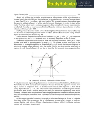

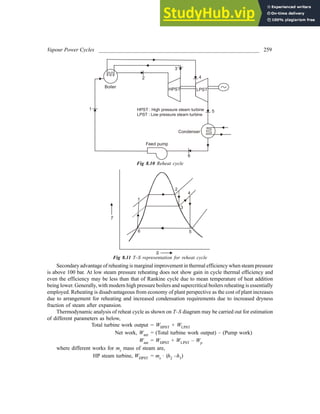


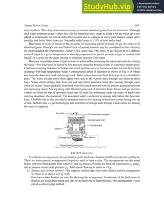


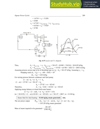


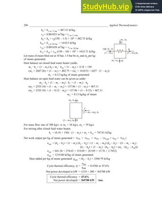


![Vapour Power Cycles ___________________________________________________________ 301
Thermal efficiency η =
add
net
w
q = 0.4503 or 45.03%
% Increase in thermal efficiency due to reheating =
0.4503 0.4478
0.4478
−
× 100
= 0.56%
Thermal efficiency of reheat cycle = 45.03%
% Increase in efficiency due to reheating = 0.56% Ans.
13. In a binary vapour cycle working on mercury and steam, the mercury vapour is generated dry
saturated at 8.45 bar and expanded upto 0.07 bar in mercury turbine. The condenser or mercury cycle is
used for generating steam at 40 bar, 0.98 dry. The steam is superheated separately upto 450ºC and then
supplied into steam turbine for being expanded upto 0.075 bar. Two closed feed water heaters are used
by bleeding out steam at 8 bar and 1 bar so as to provide feed water leaving at 150ºC and 90ºC
respectively. Condensate leaves feed water heater as saturated liquid at respective pressures and is mixed
with the hot feed water leaving the respective feed heater. The turbine running on mercury has capability
of converting 85% of available heat into work. The enthalpies of mercury may be taken as,
enthalpy of dry saturated vapour at 8.45 bar = 349 kJ/kg
enthalpy after isentropic expansion to 0.07 bar = 234.5 kJ/kg
enthalpy of saturated liquid at 0.07 bar = 35 kJ/kg
Assume feed water to enter at 150ºC into mercury condenser. Neglect pump work for getting efficiency.
Determine the steam generation rate per kg of mercury and efficiency of cycle.
Solution:
For mercury cycle,
Insentropic heat drop = 349 – 234.5 = 114.5 kJ/kg Hg
Actual heat drop = 0.85 × 114.5 = 97.325 kJ/kg Hg
Heat rejected in condenser = [349 – 97.325 – 35]
= 216.675 kJ/kg
Heat added in boiler = 349 – 35 = 314 kJ/kg
For steam cycle,
Enthalpy of steam generated = hat 40 bar, 0.98 dry = 2767.13 kJ/kg
Enthalpy of steam at inlet to steam turbine h2 = h at 40 bar, 450ºC = 3330.3 kJ/kg
Entropy of steam at inlet to steam turbine, s2 = 6.9363 kJ/kg · K
Therefore, heat added in condenser of mercury cycle
= hat 40 bar, 0.98 dry – hfeed at 40 bar
= 2767.13 – 4.18 × 150 = 2140.13 kJ/kg
Therefore, mercury required per kg of steam =
2140.13
Heat rejected in condenser
= 2140.13
216.675
= 9.88 kg per kg of steam
For isentropic expansion, s2 = s3 = s4 = s5 = 6.9363 kJ/kg · K
State 3 lies in superheated region, by interpolation the state can be given by, temperature 227.07ºC at 8
bar, h3 = 2899.23 kJ/kg](https://image.slidesharecdn.com/appliedthermodynamics3rdedition-230807154336-69e627e1/85/Applied-Thermodynamics-3rd-Edition-pdf-318-320.jpg)


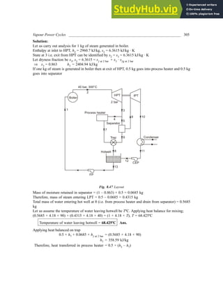
![306 _________________________________________________________ Applied Thermodynamics
= 1023.175 kJ/kg steam generated
Heat transferred per kg steam generated = 1023.175 kJ/kg steam generated Ans.
For state 10 at exit of LPT, s10 = s3 = s2 = 6.3615 kJ/kg · K
Let dryness fraction be x10
s10 = 6.3615 = sƒ at 0.075 bar + x10 · sƒg at 0.075 bar
⇒ x10 = 0.754
⇒ h10 = hf at 0.075 bar + x10 · hfg at 0.075 bar
h10 = 1982.91
Net work output, neglecting pump work per kg of steam generated,
wnet = (h2 – h3) × 1 + 0.4315 × (h3 – h10)
= 555.76 + 182.11
wnet = 737.87 kJ/kg steam generated
Heat added in boiler per kg steam generated, qadd = (h2 – h1)
= (2960.7 – 4.18 × 68.425)
qadd = 2674.68 kJ/kg
Thermal efficiency =
net
add
w
q = 0.2758 or 27.58%
Thermal efficiency = 27.58% Ans.
16. In a steam power plant operating on Rankine cycle, the steam enters the turbine at 70 bar and 550ºC
with a velocity of 30 m/s. It discharges to the condenser at 0.20 bar with a velocity 90 m/s. If the steam
flow rate is 35 kg/s, find the thermal efficiency and net power produced. [U.P.S.C. 1992]
Solution:
From steam tables, h1 = 3530.9 kJ/kg, s1 = 6.9486 kJ/kg · K
Assuming isentropic expansion in nozzle, s1 = s2 = 6.9486 kJ/kg · K
Boiler
4
1
Steam
Turbine
0.20 bar 2
Condenser
Condensate extraction
and feed pump
3
(a)
70 bar, 550°C, 35 kg/s
s
T
3 2
4
1
0.02 bar
70 bar
550°
(b)
Fig. 8.48 Schematic and representation on T-s diagram](https://image.slidesharecdn.com/appliedthermodynamics3rdedition-230807154336-69e627e1/85/Applied-Thermodynamics-3rd-Edition-pdf-323-320.jpg)

![308 _________________________________________________________ Applied Thermodynamics
The correct amount of steam is bled for feed heating at exit from the HP stage. Calculate the mass of
steam bled per kg of steam passing through the HP stage and the amount of heat supplied in the boiler
per second for an output of 10 MW. Neglect pump work, [U.P.S.C. 1993]
Solution:
Boiler
1
HPT LPT
Condenser
2
7 6
5 4
3
Feed pump
CEP
S
T
4
2
7
1
10 kPa
10 MPa
3
6
5
2 MPa
Fig. 8.49 Possible arrangement and T-s representation
From steam tables:
h1 = 3625.3 kJ/kg, s1 = 6.9029 kJ/kg · K
Due to isentropic expansion, s1 = s2 = s3 = 6.9029 kJ/kg · K
At state 2, i.e. at pressure of 2 MPa and entropy 6.9029 kJ/kg · K.
By interpolating state for s2 between 2 MPa, 300ºC and 2 MPa, 350ºC from steam tables,
h2 = 3105.08 kJ/kg
For state 3, i.e. at pressure of 0.01 MPa entropy, s3 lies in wet region as s3 < sg at 0.01 MPa. Let dryness
fraction be x3 at this state
s3 = sƒ at 0.01 MPa + x3 · sƒg at 0.01 MPa
6.9029 = 0.6493 + x3 × 7.5009
x3 = 0.834
Enthalpy at state 3, h3 = hf at 0.01 MPa + x3 · hƒg at 0.01 MPa
= 191.83 + (0.834 × 2392.8)
h3 = 2187.43 kJ/kg
Let the mass of steam bled be mb per kg of steam from exit of HP for regenerative feed heating.
Considering state at exit from feed heater being saturated liquid the enthalpy at exit of feed heater
will be, hƒ at 2 MPa.
h6 = hƒ at 2 MPa = 908.79 kJ/kg
For adiabatic mixing in feed heater, for one kg of steam leaving boiler, the heat balance yields,
(1 – mb) · h5 + mb · h2 = h6
While neglecting pump work,
h5 = h4 = hƒ at 0.01 MPa = 191.83 kJ/kg
Substituting in heat balance on the feed heater,
(1 – mb) · 191.83 + mb · 3105.08 = 908.79](https://image.slidesharecdn.com/appliedthermodynamics3rdedition-230807154336-69e627e1/85/Applied-Thermodynamics-3rd-Edition-pdf-325-320.jpg)
![Vapour Power Cycles ___________________________________________________________ 309
mb = 0.246 kg per kg of steam entering HP turbine
Steam bled per kg of steam passing through HP stage = 0.246 kg Ans.
Let mass of steam leaving boiler be m kg/s.
Output = 10 × 103 = m(h1 – h2) + m(1 – mb) (h2 – h3)
10 × 103 = m{(3625.3 – 3105.08) + (1 – 0.246) (3105.08 – 2187.43)}
m = 8.25 kg/s
Neglecting pump work, h7 = h6 = 908.79 kJ/kg
Heat supplied to boiler, Q7–1 = m(h1 – h7)
Q7–1 = 8.25 (3625.3 – 908.79)
= 22411.208 kJ/s
Heat added = 22411.21 kJ/s Ans.
18. Steam enters the first stage of a turbine at 100 bar, 500ºC and expands isentropically to 10 bar. It is
then reheated to 500ºC and expanded in the second stage to the condenser pressure of 0.1 bar. Steam is
bled from the first stage at 20 bar and fed to a closed feed water heater. Feed water leaves the closed
heater at 100 bar, 200ºC (enthalpy = 856.8 kJ/kg), while the condensate is supplied to the open heater
into which steam is bled at 4 bar pressure. Saturated liquid at 4 bar exits from the open heater and enters
the closed heater. The net output of the turbine is 50 MW. Assuming the turbine and pump processes to
be isentropic, determine the mass of steam bled at each feed water heater per kg of steam entering the
first stage, the mass of steam entering the first stage per second, and the thermal efficiency.
[U.P.S.C. 1995]
Solution:
From steam table, at inlet to first stage of turbine,
h1 = hat 100 bar, 500ºC = 3373.7 kJ/kg
s1 = sat 100 bar, 500ºC = 6.5966 kJ/kg · K
Boiler
1 kg
HPT
Condenser
5 4'
4
1 kg
LPT
FP
1 kg
9
10
7
OFWH
11
CFWH 7'
8
6
3
2
1
(1 – )
m6
(1 – – )
m m
6 8
CEP
m6
m8
m6
S
T
3
2
4
100 bar
0.1 bar
500 °C
20 bar
10 bar
4 bar
4'
11
10
5 9
7
8
6
1
7'
Fig. 8.50 Arrangement and T-s representation](https://image.slidesharecdn.com/appliedthermodynamics3rdedition-230807154336-69e627e1/85/Applied-Thermodynamics-3rd-Edition-pdf-326-320.jpg)


![328 _________________________________________________________ Applied Thermodynamics
8.9 Compare performance of regenerative cycle with simple Rankine cycle.
8.10 What do you understand by binary vapour power cycles?
8.11 Discuss advantages of binary vapour cycles over single vapour cycle.
8.12 What is mixed pressure turbine?
8.13 Describe pass out turbines and back pressure turbines.
8.14 Discuss briefly the factors limiting thermal efficiency of a steam power plant.
8.15 Describe combined heat and power cycles.
8.16 A steam engine working on Rankine cycle operates between 1.96 MPa, 250ºC and 13.7 kPa. If engine
consumes steam at the rate of 0.086 kg per second, determine Rankine cycle efficiency, neglecting
pump work. Also, find Rankine cycle efficiency considering pump work. [58.8%]
8.17 In a steam power plant working on boiler pressure of 80 bar and condenser pressure of 0.075 bar
determine cycle efficiency considering it to work on Carnot cycle. [44.9%]
8.18 A reheat cycle operates between 80 bar and 0.075 bar. Temperature of steam entering turbine is 600ºC
and first stage of expansion is carried out till the steam becomes dry saturated. Subsequently steam is
reheated upto the initial temperature at inlet. Neglecting pump work determine efficiency and specific
steam consumption in kg/hp·hr. [42.5%, 141 kg/hp-hr]
8.19 A steam turbine installation of 60 MW capacity has steam entering turbine at 7 MPa, 500ºC with steam
bleeding at 2 MPa and 0.2 MPa for feed heating. Remaining steam at 2 MPa is reheated upto 480ºC.
Steam finally leaves turbine at 36 mm Hg (absolute). Give layout, mass fraction of steam bled out per
kg of steam generated, cycle efficiency and mass flow rate of steam entering turbine.
[0.159, 0.457, 46.58 kg/s]
8.20 In a steam turbine steam enters at 1.4 MPa, 320ºC and exhausts at 175 kPa. Determine the steam flow
rate considering turbine internal efficiency of 70% and load requirement of 800 kW. [2.6 kg/s]
8.21 During trial of turbine in steam power plant the steam is found to enter turbine at 2.1 MPa, 260ºC with
flow rate of 226 kg/s. Mechanical efficiency is 95% and turbine output is 100 MW. The exhaust
pressure is 140 kPa and condensate temperature is 70ºC.
Unfortunately the old boiler fails and is to be replaced by another boiler generating steam at 4.9 MPa,
320ºC. This unit may drive an additional turbine with an internal efficiency of 90% which exhausts at
2.1 MPa. A part of exhaust is reheated to above trial conditions, including flow rate and remainder
heats feed water to 205ºC. Determine (a) total plant output, (b) new total steam flow rate, kg/s, (c) old
turbine internal efficiency, (d) the overall thermal efficiency. [14.9 MW, 293 kg/s, 94.3%, 22.9%]
8.22 A steam turbine has steam entering at 40 bar, 450ºC and leaving at 0.06 bar. Turbine develops 4000 hp
at 3000 rpm with expansion occurring in two stages and reheating in between at 2 bar and both stages
give equal output. The stages have efficiency ratio of 0.8. Determine thermal efficiency of cycle.
[32.2%]
8.23 A regenerative cycle has steam supplied at 28 bar, 300ºC in first stage. A steam fraction is bled out at
3 bar for feed heating. The feed heater drains are pumped into feed line downstream of heater at the
same temperature as the bled steam. The steam expansion may be considered isentropic throughout.
Condenser works at 0.15 bar. Determine mass of steam bled per kg of steam generated and thermal
efficiency. Also give layout and T-s diagram. [0.143 kg/kg steam generated, 31.2%]
8.24 A steam power plant has steam generated at 140 bar, 400ºC and throttled to 70 bar before supplied to
turbine. Steam expands isentropically to the pressure of 15 bar and at this pressure some quantity of
steam is bled out for feed heating which leaves as condensate at 40ºC. Remaining steam is reheated at
constant pressure by mixing it with the throttled steam taken from boiler in such amount that the
resultant mixture has temperature of 250ºC. This mixture then expands isentropically upto condenser](https://image.slidesharecdn.com/appliedthermodynamics3rdedition-230807154336-69e627e1/85/Applied-Thermodynamics-3rd-Edition-pdf-345-320.jpg)
![Vapour Power Cycles ___________________________________________________________ 329
pressure of 0.075 bar. Determine horse power developed by turbine for steam generation rate of 50
ton/hr. Also give layout and T-s diagram. [14400 hp]
8.25 Steam is required for process heating at 3 bar, dry saturated along with power output of 1 MW. A back
pressure turbine with 70% internal efficiency is used for this purpose. For the steam supplied at the
rate of 2.78 kg/s determine the pressure and temperature of steam to be generated from boiler.
[37.3 bar, 344ºC]
8.26 A steam turbine has steam being generated at 30 bar, 400ºC for being expanded upto 0.04 bar with
bleeding of some steam at 3 bar for feed heating in closed feed water heater. Feed water leaves feed
heater at 130ºC and the condensate leaving feed heater as saturated liquid is sent to drain cooler
where it gets cooled to 27ºC and finally discharged in hotwell. Condensate from condenser is also
discharged in hotwell from where feed water is picked by a pump and passed through drain cooler and
subsequently closed feed water heater. Assuming no losses and negligible pump work determine the
thermal efficiency of cycle and mass of steam bled out per kg of steam generated. Draw layout and T-
s diagram. [38.82%, 0.167 kg/kg steam]
8.27 In a steam turbine plant steam enters turbine at 20 bar, 250ºC and leaves at 0.05 bar. During expansion
some amount of steam is bled out at 5 bar, 1.5 bar and 0.3 bar for feed heating in closed feed water
heaters. Condensate leaves each feed heater as saturated liquid and is passed through traps into next
feed heater at lower pressure. Combined drain at 0.3 bar is cooled in drain cooler upto condenser
temperature and then put into hot well which also collects condensate coming from condenser,
Determine,
(a) the masses of steam bled per kg of steam generated
(b) the thermal efficiency of cycle
(c) the net work output per kg of steam generated
(d) the layout and T-s diagram. Neglect pump work.
[0.088 kg, 0.0828 kg, 0.046 kg, 35.63%, 807 kJ/kg ]
8.28 A binary vapour power cycle works on mercury and steam such that dry saturated mercury vapour at
4.5 bar is supplied to mercury turbine and leaves at 0.04 bar. Steam is generated as dry saturated at 15
bar and supplied to steam turbine for being expanded upto condenser pressure of 0.04 bar. Determine
thermal efficiency of cycle. For mercury take,
hƒ at 4.5 bar = 62.93 kJ/kg, hg at 4.5 bar = 355.98 kJ/kg,
vf at 0.04 bar = 0.0000765 m3
/kg
hƒ at 0.04 bar
= 29.98 kJ/kg, hg at 0.04 bar
= 329.85 kJ/kg
sg at 4.5 bar = 0.5397 kJ/kg · K, sg at 0.04 bar = 0.6925 kJ/kg · K,
sƒ at 0.04 bar = 0.0808 kJ/kg · K](https://image.slidesharecdn.com/appliedthermodynamics3rdedition-230807154336-69e627e1/85/Applied-Thermodynamics-3rd-Edition-pdf-346-320.jpg)


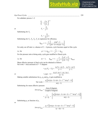


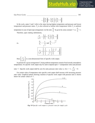


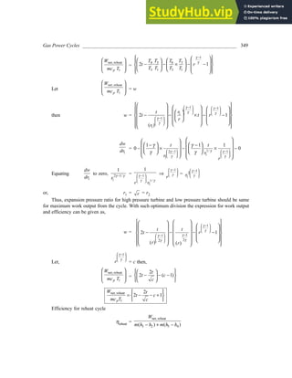


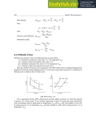


![372 _________________________________________________________ Applied Thermodynamics
Using adiabatic formulations
1
5
4
V
V
γ −
′
=
4
5
'
T
T
{here V5 = V1}
or T5 = 2929.5 ×
0.4
0.172
1.06
T5 = 1415.4 K
Heat rejected in process 5 – 1, Q5–1 = cv (T5 –T1)
= 0.71 (1415.4 – 373.15)
Q5–1 = 739.99 kJ
Efficiency of mixed cycle =
1700 739.99
1700
−
= 0.5647 or 56.47%
ηOtto cycle = 50.83%; ηmixed cycle = 56.47% Ans.
4. In an air standard Brayton cycle the minimum and maximum temperature are 300 K and 1200 K,
respectively. The pressure ratio is that which maximizes the net work developed by the cycle per unit mass
of air flow. Calculate the compressor and turbine work, each in kJ/kg air, and thermal efficiency of the
cycle. [U.P.S.C. 1994]
Solution:
Maximum temperature, T3 = 1200 K
Minimum temperature, T1 = 300 K
Optimum pressure ratio for maximum work output,
rp =
2( 1)
max
min
T
T
γ
γ −
rp =
2( 1)
3
1
T
T
γ
γ −
rp = 11.3
2
1
p
p = rp = 11.3, For process 1–2,
2
1
T
T =
1
2
1
−
P
T
γ
γ
T2 = 300 · ( )
1.4 1
1.4
11.3
−
T2 = 600.21 K
For process 3–4,
3
4
T
T
=
1
3
4
P
P
γ
γ
−
=
1
2
1
P
P
γ
γ
−
, ⇒ T4 = 599.79 K](https://image.slidesharecdn.com/appliedthermodynamics3rdedition-230807154336-69e627e1/85/Applied-Thermodynamics-3rd-Edition-pdf-389-320.jpg)
![Gas Power Cycles ______________________________________________________________ 373
Heat supplied, Q23 = cp (T3 – T2) = 602.79 kJ/kg
T
S
P = P
2 3
3
2
1
4
P = P
1 4
Fig. 9.33
Compressor work, WC = cp ·(T2 – T1) = 1.005 × (600.21 – 300) = 301.71 kJ/kg
Turbine work WT = cp · (T3 – T4) = 1.005 (1200 – 599.79) = 603.21 kJ/kg
Thermal efficiency =
Net work
Heat supplied =
23
T c
W W
Q
−
=
603.21– 301.71
602.79
= 0.5002
Compressor work = 301.71 kJ/kg, Turbine work = 603.21 kJ/kg,
Thermal efficiency = 50.02% Ans.
5. A gas turbine unit receives air at 1 bar, 300 K and compresses it adiabatically to 6.2 bar. The
compressor efficiency is 88%. The fuel has a heating value of 44186 kJ/kg and the fuel-air ratio is
0.017 kg fuel/kg of air. The turbine internal efficiency is 90%. Calculate the work of turbine and
compressor per kg of air compressed and thermal efficiency. For products of combustion cp = 1.147 kJ/
kg K, γ = 1.33. [U.P.S.C. 1992]
Solution:
Gas turbine cycle is shown by 1–2–3–4 on T-S diagram,
Given:
P1 = 1 bar, P2 = P3 = 6.2 bar, F/A ratio = 0.017
T1 = 300 K, ηcompr. = 88%, ηturb = 90%
Heating value of fuel = 44186 kJ/kg
For process 1–2 being isentropic,
2
1
T
T =
1
2
1
P
P
γ
γ
−
T2 = 505.26 K
Considering compressor efficiency, ηcompr =
2 1
2 1
'
T T
T T
−
− , 0.88 =
2
(505.26 300)
( 300)
'
T
−
−
Actual temperature after compression, T'
2 = 533.25 K
During process 2–3 due to combustion of unit mass of air compressed the energy balance shall be as
under,
Heat added = mf × Heating value
Fig. 9.34
T
S
6.2 bar
3
2
1
4
1 bar
2'
4'
300 K](https://image.slidesharecdn.com/appliedthermodynamics3rdedition-230807154336-69e627e1/85/Applied-Thermodynamics-3rd-Edition-pdf-390-320.jpg)
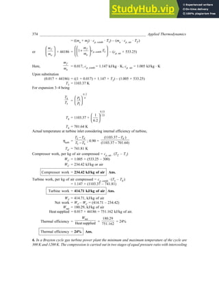


![Gas Power Cycles ______________________________________________________________ 377
3(1 )
2
p
r
γ
γ
−
=
1
5 isen,c isen, T
·
T
T η η ⇒ rp =
2
3(1 )
1
5 isen, c isen, T
.
·
T
T
γ
γ
η η
−
rp, opt =
2
3(1 )
1
5 isen, c isen, T
·
T
T
γ
γ
η η
−
Substituting known values,
rp, opt =
2 1.4
3(1 1.4)
300
1200 0.85 0.90
×
−
× ×
= 13.6
Overall optimum pressure ratio = 13.6 Ans.
7. An air compressor has eight stages of equal pressure 1.35. The flow rate through the compressor and
its’ overall efficiency are 50 kg/s and 82% respectively. If the air enters the compressor at a pressure of
1 bar and temperature of 313 K, determine;
(i) State of air at the exit of compressor
(ii) Polytropic or small stage efficiency
(iii) Efficiency of each stage
(iv) Power required to drive the compressor assuming overall efficiency as 90%.
[U.P.S.C. 1992]
Solution:
(i) Theoretically state of air at exit can be determined by the given stage pressure ratio of 1.35. Let
pressure at inlet to first stage be P1 and subsequent intermediate pressure be P2, P3, P4, P5, P6, P7, P8,
and exit pressure being P9.
Therefore,
2
1
P
P =
3 5 6 7 8 9
4
2 3 4 5 6 7 8
P P P P P P
P
P P P P P P P
= = = = = = = 1.35
or
9
1
P
P
= (1.35)8 = 11.03
Theoretically, the temperature at exit of compressor can be predicted considering isentropic compression
of air (γ = 1.4)
9
1
T
T =
1
9
1
P
P
γ
γ
−
= ( )
0.4
1.4
11.03
T9 = 621.9 K
Considering overall efficiency of compression 82% the actual temperature at compressor exit can be
obtained
9 1
9, actual 1
T T
T T
−
−
= 0.82](https://image.slidesharecdn.com/appliedthermodynamics3rdedition-230807154336-69e627e1/85/Applied-Thermodynamics-3rd-Edition-pdf-394-320.jpg)


![394 _________________________________________________________ Applied Thermodynamics
Thus, efficiency is seen to increase in combined cycle upto 57.77% as compared to gas turbine offering
48.21% efficiency.
Overall efficiency = 57.77%
Steam per kg of air = 0.119 kg steam/kg air Ans.
16. In an I.C. engine operating on the dual cycle (limited pressure cycle), the temperature of the working
fluid (air) at the beginning of compression is 27ºC. The ratio of the maximum and minimum pressures of
the cycle is 70 and the compression ratio is 15. The amount of heat added at constant volume and at
constant pressure are equal. Compute the air standard thermal efficiency of the cycle. State three main
reasons why the actual thermal efficiency is different from the theoretical value.
[U.P.S.C. 1993]
Solution:
T1 = 27ºC = 300 K
4
1
P
P
=
3
1
P
P
= 70
Compression ratio, 1
2
V
V
= 15 =
1
3
V
V
Heat added at constant volume = Heat added at constant pressure
Q23 = Q34
m · cv(T3 – T2) = m · cp·(T4 – T3)
(T3 – T2) = γ ·(T4 – T3)
For process 1–2;
2
1
T
T =
1
2
1
P
P
γ
γ
−
2
1
T
T =
1
1
2
V
V
γ −
2
300
T
= (15)0.4
T2 = 886.25
and
2
1
P
P
=
1
2
V
V
γ
= (15)1.4
P2 = P1 · (15)1.4
P2 = 44.3 P1
For process 2–3
2
3
P
P =
2
3
T
T
Fig. 9.46
V
P
1
5
4
3
2](https://image.slidesharecdn.com/appliedthermodynamics3rdedition-230807154336-69e627e1/85/Applied-Thermodynamics-3rd-Edition-pdf-411-320.jpg)
![396 _________________________________________________________ Applied Thermodynamics
Air standard thermal efficiency = 0.6529
Air standard thermal efficiency = 65.29% Ans.
Actual thermal efficiency may be different from theoretical efficiency due to following reasons;
(a) Air standard cycle analysis considers air as the working fluid while in actual cycle it is not air
throughout the cycle. Actual working fluid which are combustion products do not behave as
perfect gas.
(b) Heat addition does not occur isochorically in actual process. Also combustion is accompanied by
inefficiency such as incomplete combustion, dissociation of combustion products, etc.
(c) Specific heat variation occurs in actual processes where as in air standard cycle analysis specific
heat variation is neglected. Also during adiabatic process theoretically no heat loss occurs while
actually these processes are accompanied by heat losses.
-:-4+15-
9.1 What do you mean by air standard cycles? Discuss its’ significance.
9.2 Derive the expression for Carnot cycle efficiency.
9.3 Discuss limitations of Carnot cycle and explain Otto cycle, Diesel cycle and Dual cycle in light of these
limitations.
9.4 Derive expression for efficiency of Otto cycle, Dual cycle and Diesel cycle.
9.5 What is meant by mean effective pressure? Discuss its’ relevance.
9.6 Obtain expressions for mean effective pressure of Otto cycle, Diesel cycle and Dual cycle.
9.7 Discuss gas turbine cycles. Obtain efficiency of Brayton cycle.
9.8 What are possible modifications in gas turbine cycle? Explain.
9.9 Explain different irreversibilities and losses in gas turbine cycle.
9.10 Define polytropic efficiency and its significance mathematically for compressors.
9.11 Obtain optimum pressure ratio condition for minimum compressor work requirement in two stage
perfect intercooled compression.
9.12 Compare the influence of reheating, regeneration and intercooling on performance of gas turbine
cycle.
9.13 Discuss Ericsson cycle and obtain its efficiency.
9.14 Obtain efficiency of Stirling cycle.
9.15 Write short notes on compressor and turbine efficiencies.
9.16 An Otto cycle operates between maximum and minimum pressures of 600 kPa and 100 kPa. The
minimum and maximum temperatures in the cycle are 27ºC and 1600 K. Determine thermal efficiency of
cycle and also show it on T-s and P-V diagram. [48%]
9.17 In an air standard Carnot cycle operating between temperatures of 57ºC and 1327ºC, determine the
heat added if cycle efficiency is 79.4% and the minimum pressure of cycle is 100 kPa. [300 kJ/kg]
9.18 Determine air standard efficiency for a diesel engine having L/D ratio of 1.6 and bore as 25 cm. Take the
clearance volume and pressure at end of suction as 1.2 litres and 1 atm. respectively. Also obtain mean
effective pressure. Volume after combustion is 1.8 times clearance volume. [63.5, 6 bar]
9.19 An engine operates on Dual cycle with a compression ratio of 15. At the end of suction the air is
available at 1 atm and 27ºC. Total heat added is 430 kJ/kg. Heat supply is in ratio of (0.536:1) for heat
supply at constant volume and constant pressure. Determine cycle efficiency and mean effective
pressure. [65%, 0.342 MPa]
9.20 A regenerative cycle has heat exchanger effectiveness of 75% and pressure ratio of 4 with compression
occurring in two stages of equal pressure ratio with intercooling back to initial temperature of 15ºC.
Maximum temperature in cycle is 650º C and expansion occurs with efficiency of 0.88. Compression
process has isentropic efficiency of 0.85 in each stage. Considering air as working fluid throughout
the cycle determine efficiency of cycle. [34.6%]](https://image.slidesharecdn.com/appliedthermodynamics3rdedition-230807154336-69e627e1/85/Applied-Thermodynamics-3rd-Edition-pdf-413-320.jpg)
![Gas Power Cycles ______________________________________________________________ 397
9.21 A gas turbine installation has intercooling, regeneration and reheating with air entering compressor at
100 kPa, 290 K and compressed to 0.41 MPa. Subsequently it is cooled until temperature drops to 13ºC
in intercooler and finally compressed to 0.75 MPa. Regenerator effectiveness is 0.70 and turbine inlet
temperature (TIT) is 1350 K and expands to 0.41 MPa where it is reheated upto 1350 K. The exhaust
pressure is 0.1 MPa. Determine overall efficiency considering expansion and compression processes
to be of isentropic type. Take air as working fluid throughout. [54.3%]
9.22 In an actual gas turbine the compressor requires 300 kJ/kg of work to quadruple the inlet pressure. For
inlet air temperature of 100ºC determine, the compressor exit air temperature and compressor efficiency.
[671.6 K, 60.6%]
9.23 In a gas turbine installation the exhaust from gas turbine is sent for process heating at 200 kPa.
Turbine produces power just sufficient to drive the compressor. Turbine inlet temperature is 815ºC
and air is supplied to compressor at 1 bar, 17ºC. Determine compressor pressure ratio for air as working
fluid throughout. [3]
9.24 A Brayton cycle producing 75 kW is designed for maximum work. The compressor inlet conditions are
100 kPa and 27ºC. Compression ratio is 5.5. For air standard Brayton cycle determine the turbine inlet
temperature, cycle efficiency and air flow rate. [794 K, 38.6%, 0.631 kg/s]
9.25 A gas turbine cycle has reheating and heat exchanger employed. The air is supplied at 1 bar, 15ºC into
compressor where it is compressed upto 4 bar with isentropic efficiency of 82%. Turbine inlet
temperature is 700ºC and expansion occurs in two stages with equal pressure ratio upto 1 bar. The
reheating between two stages occurs upto 700ºC. Isentropic efficiency of expansion is 85%. Exhaust
from low pressure turbine is passed into a heat exchanger having 0.75 effectiveness. Heat exchanger
heats the discharge from compressor before being supplied to combustion chamber. Considering air
as woking fluid throughout determine cycle efficiency. [32.1%]
9.26 In a gas turbine plant air is supplied at 1 bar, 290 K to compressor having isentropic efficiency of 0.84
and pressure ratio of 5. The air flow rate to compressor is 111600 kg/hr. Compressed air is passed
through a heat exchanger and it leaves exchanger at 360ºC, from where it is supplied to combustion
chamber. Fuel having calorific value of 41800 kJ/kg is supplied at the rate of 890 kg/hr in combustion
chamber. The combustion products expand from 4.7 bar to 1.95 bar, 410ºC in turbine. Take cp air = 1.0032
kJ/kg K, γair = 1.4, cp comb, products = 1.1286 kJ/kg K, γcomb, products = 1.34. Determine hp developed.
[3000 hp]
9.27 Show that the necessary condition for positive work output from an open cycle gas turbine can be
given by,
ηc × ηT × Tmax > Tmin .
1
r
γ
γ
−
The simple gas turbine cycle has compressor with isentropic efficiency of ηc and pressure ratio of ‘r’.
Turbine has isentropic efficiency of ηT and expansion ratio similar to that of compressor. The maximum
and minimum temperature are Tmax and Tmin and air is working fluid throughout with γ as ratio of
specific heat.
9.28 In a gas turbine installation based on Brayton cycle the highest and lowest temperatures are
TH and TL respectively. The pressure ratio and heat input from high temperature reservoir
vary such that temperature TH and TL remain constant. Show that the expression for net
maximum work output is, Wmax =
2
. 1
H
P L
L
T
C T
T
−
.
9.29 A gas turbine installation has double stage compressor and double stage turbine having
pressure ratio across each stage as 8:1 in both compressor and turbine. Pressure at inlet to
compressor is 1 bar and temperature entering each compressor is 293K and temperature](https://image.slidesharecdn.com/appliedthermodynamics3rdedition-230807154336-69e627e1/85/Applied-Thermodynamics-3rd-Edition-pdf-414-320.jpg)
![398 _________________________________________________________ Applied Thermodynamics
entering each turbine is 1373K. Considering ideal regenerator in cycle determine cycle
thermal efficiency and turbine work output.
[0.613, 1.235 MJ/kg]
9.30 An ideal Stirling cycle running on hydrogen works between temperature of 723°C and 23°C
while highest and lowest pressure are 30 bar and 5 bar respectively. Considering it to be
closed cycle determine the heat transfer to regenerator per cycle, net work per cycle and
cycle efficiency.
[3.67 MJ, 0.85 MJ, 70%]
9.31 An ideal Eriscsson cycle is running on helium. Helium is at 1.5 bar, 500°C at the start of
compression process and expansion process occurs at a pressure of 35 bar. Temperature
of low temperature reservoir is 298 K. Determine the thermal efficiency and net work of
cycle.
[61.5%, 31.075MJ]
9.32 Determine thermal efficiency of cycle, backwork ratio and net power produced from a gas
turbine installation having compressor admitting air at 1 bar, 300K & 5 m3
/s volume
flow rate. Air is compressed in two stages up to 12 bar with intercooling to 300K between
stages at a pressure of 350 kPa. Turbine inlet temperature is 1127 °C and expanssion occurs
in two stages with reheat to 1340K between stages at a pressure of 3.5 bar. Compressor
and turbine stage efficiencies are 87% and 85% respectively. Also find the % gain in
efficiency if a regenerator with effectiveness of 80% is employed in plant. Show the process
on T-S diagram.
[29.8%, 0.441, 2.17 MW, 59.66%]
9.33 A gas turbine runs at pressure ratio of 7 and maximum temperature of 1000K. Air enters
compressor at temperature of 288 K. The isentropic efficiency of turbine and compressor
are 90% & 85% respectively. Find the percentage reduction in efficiency compared to ideal
Brayton cycle. Also find net work output and back work ratio of gas turbine. Show the
processes on T-S diagram. [32.85%, 132.5 kJ/kg, 0.656]](https://image.slidesharecdn.com/appliedthermodynamics3rdedition-230807154336-69e627e1/85/Applied-Thermodynamics-3rd-Edition-pdf-415-320.jpg)


![Fuels and Combustion __________________________________________________________ 407
In any fuel containing carbon (C), hydrogen (H2), oxygen (O) and sulphur (S) the higher calorific
value of fuel can be estimated using respective calorific values for constituents. In the fuel oxygen is not
present in free form but is associated with hydrogen.
H2 + O ® H2O
(2) (16) (18)
On mass basis, 1 kg (H2) + 8 kg (O) ® 9 kg (H2O)
1
8
kg (H2) + 1 kg (O) ®
9
8
kg (H2O)
Above chemical equation indicates that with every unit mass of oxygen,
1
8
of oxygen mass shall be
the mass of hydrogen associated with it. Thus, the free hydrogen available for oxidation (combustion)
shall be only H
O
-
8
e j where H refers to hydrogen mass and O refers to oxygen mass.
The higher calorific value of fuel can thus be given as under using the mass fractions of constitu-
ent elements known. If percentage mass fractions of fuel constituents are given by C, H, O and S then.
H.C.V. of fuel =
1
100
[8100·C + 34,400 H
O
-
8
e j + 2220·S] kcal/kg
Lower calorific value of fuel can be given by,
L.C.V. of fuel = (H.C.V. of fuel) – (Heat carried by water vapour formed per kg of fuel burnt)
The amount of latent heat carried depends upon the pressure at which evaporation takes place
and quantity of water vapour formed. Generally, the evaporation is considered to take place at saturation
temperature of 15°C and the latent heat of water vapour at this saturation temperature is 588.76 kcal/kg.
During combustion of fuel the water shall be formed due to hydrogen present in fuel, therefore mass of
water vapour can be given by the mass fraction of hydrogen. Thus,
L.C.V. of fuel = H.C.V. of fuel
H
( ) -
´ ´
FH IK
9 588 76
100
.
{ }, kcal/kg
10.7 COMBUSTION ANALYSIS
From earlier discussions it is seen how the combustion of a fuel can be written in the form of chemical
reactions for the oxidation of different elements constituting fuel. Based on chemical reactions the mass
of oxygen required per kg of element can be estimated. From these the oxygen requirement per kg of
fuel constituents and subsequently mass of air required for the estimated oxygen requirement can be
known. Let us see how air required for complete burning of a fuel having 85.5% carbon, 12.3%
hydrogen and 2.2% ash is calculated;
Mass of oxygen required for constituents;
1 kg of carbon shall require
8
3
kg of oxygen
1 kg of hydrogen shall require 8 kg of oxygen
Ash shall not undergo oxidation.](https://image.slidesharecdn.com/appliedthermodynamics3rdedition-230807154336-69e627e1/85/Applied-Thermodynamics-3rd-Edition-pdf-424-320.jpg)


![414 _________________________________________________________ Applied Thermodynamics
Solution:
Combustion equation for the coal (100 kg of coal) can be given as under;
86
12
C
6
1
H
5
16
O
2
14
N
1
32
S
× + × + × + × + ×
FH IK + n(O2 + 3.76 N2) ®
a × CO2 + b × SO2 + d × N2 + e × H2O
From above equation C, H, O, S, N can be equated on both the sides as under,
C; 7.16 = a
H; 6 = 2e
O; (0.3125 + 2n) = 2a + 2b + e
N; (0.1429 + 3.76 ´ 2n) = 2d
S; 0.03125 = b
Solving we get a = 7.16
b = 0.03125
d = 32.163
e = 3
n = 8.535
Amount of air required shall be [8.535 ´ (4.76)] kg mol per 100 kg of coal.
Air-fuel ratio =
8 4 76 28
100
.535 . .97
´ ´
= 11.77 kg air per kg of fuel
Air-fuel ratio = 11.77 Ans.
2. One kg C8H18 fuel is supplied to an engine with 13 kg of air. Determine the percentage by
volume of CO2 in dry exhaust gas considering exhaust gas to consist of CO2, CO and N2.
Solution:
Combustion equation in mol. basis for one kg of fuel supplied shall be as under.
1
114
(C8H18) + n(0.21 O2 + 0.79 N2) “ ® a × CO2 + b × CO + d × N2 + e × H2O
Equating the coefficients on both sides,
C;
8
114
= 0.0702 = a + b
O2; 0.21 n = a +
b e
2 2
+
H;
18
114
= 0.1579 = 2e
N2; 0.79 n = d. Also it is given that 13 kg of air per kg of fuel is supplied, therefore
n =
13
28.97
= 0.4487
Solving above following are available,
a = 0.0393
b = 0.0309](https://image.slidesharecdn.com/appliedthermodynamics3rdedition-230807154336-69e627e1/85/Applied-Thermodynamics-3rd-Edition-pdf-431-320.jpg)


![Fuels and Combustion __________________________________________________________ 433
It yields,
a = 1
b = 22.56
d = 2
e = 4
Now the combustion equation with 200% excess air shall be;
With 200% excess air; Ans.
CH4 + 6(O2 + 3.76N2) ® CO2 + 22.56N2 + 2H2O + 4O2
When there is 20% less air then actual air supplied will be 20% less than 100% theoretical air. Due
to less than theoretical air supplied there will be incomplete combustion and CO will be present with
combustion products.
CH4 + 0.8 ´ 2 (O2 + 3.76N2) ® aCO2 + bCO + dN2 + eH2O
Equating C, H2, O2 and N2 we get
C; a + b = 1
O2; a +
b e
2 2
+ = 1.6
H2; e = 2
N2; d = 1.2 ´ 3.76 = 4.512
It yields,
a = 0.2
b = 0.8
d = 4.512
e = 2
Hence for 20% less air the combustion equation shall be as under
For 20% less air.
CH4 + 1.6 (O2 + 3.76N2) ® 0.2CO2 + 0.8CO + 4.512N2 + 2H2O Ans.
16. Determine the adiabatic flame temperature for the combustion of carbon monoxide (CO) with
150 percent theoretical amount of oxygen to form CO2. The reactants enter the steady flow reactor at
25°C, 1 atm and the products are CO2 and excess O2. Enthalpy of O2, CO and CO2 are 0 kJ/kg mole,
– 110418 kJ/kg and – 393,137 kJ/kg mole respectively. The constant pressure specific heats of CO2 and O2
at 1 atm, may be assumed to be 56.43 and 36.5 kJ/kg mole K, respectively.[U.P.S.C. 1993]
Solution:
Combustion equation of carbon monoxide yields,
2CO +
3
2
O2 ® 2CO2 +
1
2
O2
Since the process is adiabatic so the total enthalpy of reactants and products shall remain same,
Enthalpy of reactants = 2 (– 110,418) +
1
2
(0)
= – 220,836 kJ/kg × mole](https://image.slidesharecdn.com/appliedthermodynamics3rdedition-230807154336-69e627e1/85/Applied-Thermodynamics-3rd-Edition-pdf-450-320.jpg)
![434 _________________________________________________________ Applied Thermodynamics
Enthalpy of products for adiabatic flame temperature to be T°K.
= [2 (– 393,137) + (56.43 × (T – 298)) + (
1
2
× 36.5 × (T – 298))]
Enthalpy of reactants = Enthalpy of products
– 220,836 = [2 × (– 393,137) + (56.43 × (T – 298)) + (
1
2
× 36.5 × (T – 298))}
T = 7869.48 K
. Adiabatic flame temperature = 7869.48 K Ans
-:-4+15-
10.1 What do you understand by fuel?
10.2 Describe different types of fuel.
10.3 What do you mean by endothermic and exothermic reactions? Explain.
10.4 Describe proximate analysis and ultimate analysis and their relevance.
10.5 What is meant by stoichiometric air-fuel ratio?
10.6 Describe calorific values of fuel and its’ measurement.
10.7 What is excess air?
10.8 Explain working of Orsat analyzer for flue gas analysis.
10.9 Describe fuel cells.
10.10 Define adiabatic flame temperature.
10.11 A coal sample has 90% carbon, 3.3% hydrogen, 3% oxygen, 0.8% nitrogen. 0.9% sulphur and 2%
ash. For 50% excess air supply determine percentage composition of dry flue gases by volume
and minimum oxygen required.
[13% CO2, 7.1.% O2, 80% N2, minimum oxygen = 2.64 kg]
10.12 A coal sample has 85% carbon, 6% hydrogen, 6% oxygen and 3% ash by mass. What will be the
minimum quantity of air required per kg of coal? Take air to have 23% O2 and 77% N2 by mass.
[11.70 kg]
10.13 For a hydrocarbon fuel having 84.8% carbon, 15.2% hydrogen by mass determine the
stoichiometric air-fuel ratio. Also obtain the volumetric composition of combustion products with
15% excess air being supplied. [15.11, 12.51% CO2, 2.89% O2, 84.60% N2]
10.14 For a coal fuel sample having 86% carbon, 4% hydrogen, 4.5% oxygen and 5.5% ash by mass
determine minimum air required per kg of coal. Also find volumetric composition of combustion
products when the actual air supplied for combustion is 1.5 times the minimum air required for
complete combustion.
[11.16 kg air/kg of fuel, 12.52% CO2, 80.47% N2, 7.01% O2]
10.15 During the combustion of coal having 22% carbon, 3.5% hydrogen, 6.5% oxygen and remaining
ash by mass, the dry flue gas has volumetric composition of 8% CO2, 1.5% CO, 80.5% N2 and
10% O2. Calculate the minimum air required per kg of coal and % excess air. Consider air to have
23% and 77% of oxygen and nitrogen respectively by mass. [3.48 kg air, 43.3% excess air]
10.16 A liquid fuel has 86% C and 14% H2 by mass. During combustion actual air supplied is 10% less
than the theoretically required for complete combustion. Obtain the volumetric composition of dry
flue gases considering that all hydrogen gets burnt and carbon gets burnt to form carbon
monoxide and carbon dioxide with no free carbon left. [11.39% CO2, 4.78% CO, 83.82% N2]](https://image.slidesharecdn.com/appliedthermodynamics3rdedition-230807154336-69e627e1/85/Applied-Thermodynamics-3rd-Edition-pdf-451-320.jpg)
![Fuels and Combustion __________________________________________________________ 435
10.17 A producer gas sample has 2% CH4, 2% O2, 14% H2, 22% CO, 5% CO2 and 55% N2 by volume.
Determine the minimum air requirement per m3
of gas and the volumetric analysis of combustion
products for 40% excess air supply. Take air to have 21% oxygen by volume.
[0.952 m3
air, 14.7% CO2, 81.25% N2, 4.05% O2]
10.18 Determine air fuel ratio and percentage excess air for a liquid fuel sample whose ultimate analysis
shows 85% carbon and 15% hydrogen. It produces dry exhaust gases having 11.5% CO2, 1.2%
CO, 0.9% O2, 86% N2 by volume after combustion. [15.07, 12.47% excess air]
10.19 C10 H22 is burnt with air fuel ratio of 13 by mass. Combustion is such that complete of hydrogen
burns into water and there is no free oxygen and no free carbon. Also the carbon dioxide and
carbon monoxide are present in combustion products. Determine volumetric analysis of
combustion products. [7.68% CO2, 6.25% CO, 15.32% H2O, 70.75% N2]
10.20 A hydrocarbon fuel has 86% carbon and 14% hydrogen. The heat evolved by 1 kg carbon burning
to CO2 is 33800 kJ and 1 kg hydrogen burning is 142000 kJ. For 25% of excess air supply determine
the mass of air required and higher calorific value. [18.52 kg air, 48948 kJ/kg fuel]
10.21 Determine air fuel ratio for combustion of C3H8 (Propane) with 200 percent theoretical air supplied.
[31.62]
10.22 Transform the volumetric analysis as given into gravimetric analysis. 15% CO, 2.2% CO, 1.6% O2,
81.2% N2. [21.6% CO2, 2.2% CO, 1.7% O2, 74.5% N2]
10.23 A coal sample has 66% C, 5.9% H2, 1% S, 19.9% O2, 1.5% N2, 5.6% ash by mass and calorific value
of 29000 kJ/kg. When this coal is burnt with 30% excess air the temperature of flue gases leaving
is 300°C and ambient temperature is 17°C. Considering combustion to be complete and partial
pressure of moisture to be 0.07 bar in flue gases and energy accompanied being 3075 kJ/kg of steam,
determine,
(i) the air-fuel ratio by mass.
(ii) the volumetric analysis of combustion products.
(iii) the heat carried away by flue gases as percentage of heat released by coal.
[11.55, 19.37% O2, 4.25% H2O, 0.16% SO2, 4.91% O2, 71.31% N2, 17.36%]
10.24 Determine the higher and lower calorific values of gas at atmospheric pressure and 15°C using
the following observations from a gas calorimeter for any fixed time.
Atmospheric pressure = 76 cm Hg
Gas burnt = 0.015 m3
Cooling water collected = 11 kg
Condensate collected = 0.01 kg
Cooling water temperature rise = 6°C
Gas pressure above atmosphere = 4.2 cm of water
Gas temperature = 17°C
Latent heat of steam at atmospheric pressure = 2440 kJ/kg
Density of mercury = 13600 kg/m3
.
[Higher calorific value = 18470 kJ/m3
, Lower calorific value = 18445.6 kJ/m3
]
10.25 Determine the net and gross calorific values per kg of mixture at constant pressure for
stoichiometric mixture of air and C6H6 (benzene) vapour at 25°C. Enthalpy of combustion for C6H6
at 25°C is – 3169500 kJ/kmol and the water is present in vapour phase in the combustion products.
[2861 kJ/kg, 2981 kJ/kg]](https://image.slidesharecdn.com/appliedthermodynamics3rdedition-230807154336-69e627e1/85/Applied-Thermodynamics-3rd-Edition-pdf-452-320.jpg)


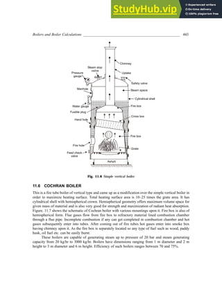


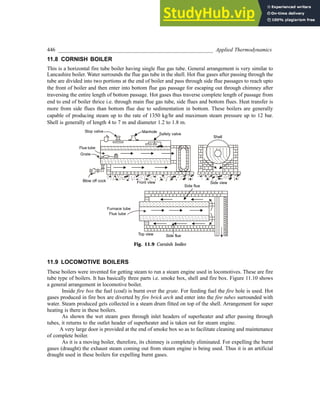


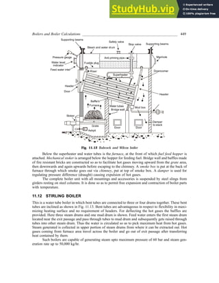
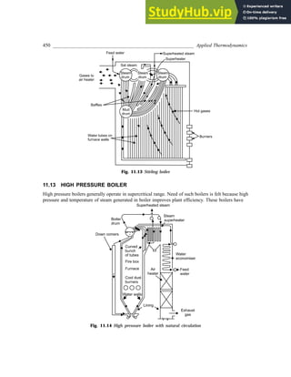


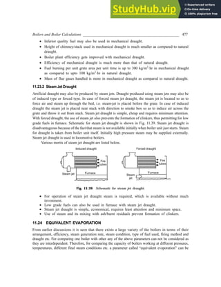


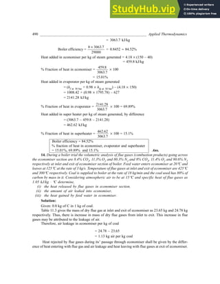
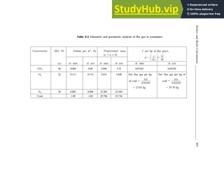


![502 _________________________________________________________ Applied Thermodynamics
Fraction of energy consumed in boiler =
18415.2
30500
= 0.6038 or 60.38% Ans.
Fracton of energy consumed in superheater =
2094.4
30500
= 0.0687 or 6.87%
-:-4+15-
11.1 Define boiler.
11.2 Classify the boilers and briefly describe each type of them.
11.3 Enlist the requirements of a good boiler.
11.4 Differentiate between fire tube and water tube boilers.
11.5 Describe briefly a vertical boiler. Also give its’ neat sketch.
11.6 Sketch and completely label a Lancashire boiler. Also explain its’ working.
11.7 Sketch and describe working of Locomotive boilers.
11.8 What do you understand by high pressure boilers?
11.9 Explain working of Bacock and Wilcox boiler.
11.10 Sketch and describe a Stirling boiler.
11.11 Sketch and describe working of Loeffler boiler.
11.12 Differentiate between mountings and accessories.
11.13 Classify mountings into safety fittings and control fittings.
11.14 Describe superheater, economiser and air preheater with neat sketches. Also indicate suitable
location of these on a boiler with line diagram.
11.15 Write short notes on, water level indicator, safety valves, fusible plug, feed check valve, pressure
gauge, stop valve and blow off cock.
11.16 Define boiler draught and also classify it.
11.17 Describe functions of chimney in a boiler.
11.18 Obtain the expression for the natural draught in terms of height of water column. Also state the
assumption made.
11.19 Derive the condition for maximum discharge through a chimney in natural draught.
11.20 Compare natural draught with artificial draught.
11.21 Describe briefly different types of mechanical draught.
11.22 Compare the power requirements for forced draught and induced draught.
11.23 Define equivalent evaporation and also give its significance.
11.24 Describe balanced draught.
11.25 What is meant by boiler trial? Explain.
11.26 Determine the height of chimney required to produce draught equivalent to 16.7 mm of water
column for the flue gases at 300°C and ambient temperature of 20°C. Take the air requirement to
be 20 kg/kg of fuel. [30 m]
11.27 Calculate the draught produced in mm of water by chimney of 35 m height, flue gas temperature
of 643 K, boiler house temperature of 307 K and air supplied at 18.8 kg per kg of coal.
[20 mm]
11.28 Show that the height of chimney required for producing a draight equivalent to 15 mm of water
can not be less than 30 m, if the flue gas temperature is 250°C, ambient temperature is 20°C and
minimum 18 kg air per kg of fuel is required.](https://image.slidesharecdn.com/appliedthermodynamics3rdedition-230807154336-69e627e1/85/Applied-Thermodynamics-3rd-Edition-pdf-519-320.jpg)
![Boilers and Boiler Calculations ___________________________________________________ 503
11.29 In a boiler installation the height of chimney is 38 m and the hot gas temperature is 570 K and
ambient air temperature is 300 K. Considering the diameter of chimney to be 2m, air/fuel ratio
being 19 determine the mass flow rate of flue gases flowing out. [3012 kg/min]
11.30 Determine the percentage of excess air supplied in a boiler where coal having 80% C, 6% moisture,
14% ash by mass is burnt inside. Hot gas temperature is 570 K and ambient air temperature is
300 K. The height of chimney is 30 m to produce draught equivalent to 1.5 cm of water column.
[20.1%]
11.31 For the maximum discharge condition through a chimney having height of 15 m determine the
draught in mm of water when ambient air temperature is 15°C. [9.2 mm]
11.32 Determine the efficiency of chimney which operates with hot gas temperature of 370°C in natural
draught and if it is operated with artificial draught the hot gas temperature drops down to 150°C.
The height of chimney is 45 m, air/fuel ratio is 24 and ambient temperature is 35°C, Take Cp for
hot gases as 1.004 kJ/kg × K. [0.2%]
11.33 In a boiler chimney the different pressure losses are measured to be as under,
Pressure loss on grate and boiler flues = 6 mm of water in each.
Pressure loss in bends and chimney duct = 2 mm of water in each.
Pressure head causing flow of hot gases = 1.2 mm of water.
Determine the height and diameter of chimney if air/coal ratio is 14, average coal consumption is
2000 kg/hr, hot gas temperature is 300°C, ambient air temperature is 310 K and actual draught is 0.8
times theoretical draught. [44.8 m, 1.6 m]
11.34 Determine the power required for a forced draught and induced draught fan in a boiler having coal
consumption of 25 kg/min and air/fuel ratio of 19 by mass. The ambient air temperature and hot
gas temperature at exit are 30°C and 140°C respectively. Draught required is equivalent to 32.2 mm
of water and mechanical efficiency of motor/fan is merely 70%. [4.16 hp, 5.97 hp]
11.35 Determine the capacity of motor required for running forced draught fan to maintain draught of
50 mm of water when the hot flue gas temperature and boiler house temperature are 175°C and
30°C respectively. The boiler has coal requirement of 25.4 kg/hr and the flue gases are produced
at the rate of 19 kg per kg of coal burnt. Considering mechanical efficiency of 78% compare the
power requirement of forced draught and induced draught arrangement.
[50.5 hp, FD requires 33% less power than 1D]
11.36 A boiler has equivalent evaporation of 1300 kg/hr from and at 100°C. The fuel consumption per
hour is 159.5 kg/hr and the boiler efficiency is 72%. Determine actual equivalent evaporation if
feed is supplied at 110°C to generate steam at 100 kg/m2
per hour and 15 bar, 200°C. Also find
calorific value of coal burnt and the grate area.
[1255 kg/hr, 25498 kJ/kg, 12.6 m2
]
11.37 Determine equivalent evaporation per kg of coal and efficiency of boiler when it consumes coal
at the rate of 52 kg/hr and steam is generated at 7 bar, 0.907 dry, 541.7 kg/hr from feed water
supplied at 40°C.
[11.075 kg per kg of coal, 83.3%]
11.38 During a boiler trial for 24 hour the following is observed;
Steam generated = 160000 kg
Mean steam pressure = 12 bar
State of steam generated = 0.85
Feed water temperature = 30°C
Coal burnt = 16000 kg](https://image.slidesharecdn.com/appliedthermodynamics3rdedition-230807154336-69e627e1/85/Applied-Thermodynamics-3rd-Edition-pdf-520-320.jpg)
![504 _________________________________________________________ Applied Thermodynamics
C.V. of coal = 33400 kJ/kg
Determine equivalent evaporation from and at 100°C and efficiency of boiler.
[10.45 kg/kg of coal, 70.65%]
11.39 A boiler has air supplied at 20°C and flue gas temperature of 220°C. The coal burnt has composition
by mass of 85% C, 3.9% H, 1.4% O and remaining ash. Volumetric composition of dry flue gas is
12.7% CO2, 1.4% CO, 4.1.% O2, 81.8% N2. The dew point temperature of wet flue gases is 50°C.
Calorific value of coal may be taken as 10157.4 kJ/kg. Take Cp of dry flue gas as 1.0032 kJ/kg × K,
Cp of superheated steam as 1.5048 kJ/kg × K.
Determine the heat carried away by dry flue gas, heat carried by moisture from combustion and
heat loss due to incomplete combustion of carbon for per kg of coal burnt.
[3080.7 kJ/kg, 969.8 kJ/kg, 2027.3 kJ/kg]
11.40 Draw heat balance sheet for a boiler whose 24 hour trial yields following;
Ambient temperature = 35°C
Coal burnt = 19200 kg, Ash collected = 1440 kg,
Combustion in ash = 54 kg, Steam generated = 198000 kg,
Moisture in coal = 2.16%,
Steam temperature = 198.9°C, Feed water temperature = 150°C, Flue gas temperature = 315°C, Coal
composition by mass = 83.39% C, 4.56% H2, 5.05% O2, 0.64% S, 1.03% N2, 5.33% ash
Flue gas analysis by volume
= 12.8% CO2, 6.4% O2, 0.2% CO, 80.6% N2
The partial pressure of steam = 0.07 bar,
Specific heat of steam = 2.0064 kJ/kg × K
[Heat supplied in steam generation = 66.62%
Heat carried by dry flue gas = 13.38%,
Heat carried by moisture = 3.76%,
Heat carried by ash = 0.28%,
Unaccounted heat = 15.96%]
11.41 Steam is generated at 100000 kg/hr from a boiler at 100 bar, 500°C with feed water supplied at
160°C. The fuel burnt in boiler has calorific value of 21000 kJ/kg and boiler efficiency is 88%.
Determine rate of fuel burnt per hour and percentage of total heat absorbed in economiser,
evaporator and superheater. [14592 kg/hr, 27.09%, 48.84%, 24.07%]
11.42 Compare the steam generation capacities of two boilers A and B for which operating parameters
are, Steam generation pressure = 14 bar, feed water temperature = 27°C, Specific heat of feed water
= 41.8 kJ/kg × K, Specific heat of steam = 2.1 kJ/kg × K,
For boiler A: State of steam = 0.9 dry
Boiler efficiency = 73%
Calorific value of coal = 34000 kJ/kg
For boiler B: State of steam = 240°C
Boiler efficiency = 79.5%
Calorific value of coal = 46000 kJ/kg
[For boiler A 10 kg/kg of coal burnt, for boiler B 14 kg/kg of coal burnt]](https://image.slidesharecdn.com/appliedthermodynamics3rdedition-230807154336-69e627e1/85/Applied-Thermodynamics-3rd-Edition-pdf-521-320.jpg)
![Boilers and Boiler Calculations ___________________________________________________ 505
11.43 A boiler generates steam at 15 bar, 0.95 dry from feed water entering at 65°C, 2040 kg/hr. Dry coal
burnt is 232 kg/hr and mean boiler house temperature is 25.3°C and flue gas temperature is 440°C.
Consider partial pressure of steam as 0.07 bar.
Composition of dry coal by mass: 83% C, 6% H2, 5% O2, 6% ash.
Composition of dry flue gas by volume: 10.50% CO2, 1.3% CO, 7.67% O2, 80.53% N2
Higher calorific value of dry coal = 34276 kJ/kg
Specific heat of dry flue gas = 0.9948 kJ/kg × K
Determine (a) total mass of flue gases per kg of coal, (b) percentage of excess air supplied, (c)
heat balance sheet per kg of dry coal
[17.58 kg/kg of coal, excess air = 49.51%, Heat taken by steam = 62.02%,Heat taken by dry flue
gas = 21.1%, Heat by moisture = 5.32%, Unaccounted = 11.56%]](https://image.slidesharecdn.com/appliedthermodynamics3rdedition-230807154336-69e627e1/85/Applied-Thermodynamics-3rd-Edition-pdf-522-320.jpg)


![Steam Engine _________________________________________________________________ 531
Fig. 12.25 Indicator diagram for compound steam engine
12.12 CALCULATIONS FOR COMPOUND STEAM ENGINES
Compound steam engine cylinders may be designed based upon the assumption of ‘equal initial piston
loads on all pistons’ or ‘equal power developed in each cylinder for getting uniform torque’ or ‘equal
temperature drop in every cylinder for optimal use of steam.
The hypothetical work output (indicator work) for HP and LP cylinders can be given as below;
Hypothetical indicator work from HP cylinder
= [p1 Vb (1 + ln rHP) – p3 × Vh]
Actual indicator work from HP cylinder
= [p1 Vb × (1 + ln rHP) – p3 × Vh] × dfHP
where rHP and dfHP are expansion ratio and diagram factor for HP cylinder. So, rHP =
V
V
h
b
Hypothetical indicator work from LP cylinder
= [p3 Vc (1 + ln rLP) – p5 × Vd]](https://image.slidesharecdn.com/appliedthermodynamics3rdedition-230807154336-69e627e1/85/Applied-Thermodynamics-3rd-Edition-pdf-548-320.jpg)
![532 ________________________________________________________ Applied Thermodynamics
Actual indicator work from LP cylinder
= [p3 Vc (1 + ln rLP) – p5 × Vd] × dfLP
where rLP and dfLP are expansion ratio and diagram factor for LP cylinder. Here rLP =
V
V
d
c
.
Total actual indicator work from compound steam engine
= [p1 Vb ( 1 + ln rHP) – p3 × Vh] × dfHP + [p3 Vc (1 + ln rLP) – p5 × Vd] × dfLP
Expansion ratio and diagram factors for two cylinders may be same or different.
Loss of work due to unresisted expansion can be quantified by the difference between total
hypothetical output and actual output from compound engine
Loss of work = Area of total hypothetical diagram – (Area of hypothetical HP diagram + Area of
hypothetical LP diagram)
= Aabdef – (Aabhog + Agcdef)
Mean effective pressures of both cylinders may be given separately or with reference to common
cylinder.
Mean effective pressure of HP cylinder
=
Area of indicator diagram for HP cylinder
Stroke volume for HP cylinder i.e.
length of diagram for HP
mepHP =
W
V
HP
HP
D
Similarly,
Mean effective pressure of LP cylinder
=
Area of indicator diagram for LP cylinder
Stroke volume for LP cylinder i.e.
length of diagram for LP
mepLP =
W
V
LP
LP
D
Mean effective pressures can be mathematically given as below,
mepHP =
p r
r
1 1 + ln HP
HP
a f – p3
mepLP =
p r
r
3 1 + ln LP
LP
a f – p5
In case of multi cylinder engines as in case of compound steam engines mean effective pressures
when defined separately offer difficulty in comparing them. Therefore, mean effective pressure is
defined in reference to LP cylinder, which means it is assumed that the stroke volume of LP cylinder is
used for all cylinders and the mean effective pressure values can be directly used for comparing work
output from respective cylinders. In case of compound engine having HP and LP cylinders the mean
effective pressure of HP cylinder referred to LP cylinder can be given as below.](https://image.slidesharecdn.com/appliedthermodynamics3rdedition-230807154336-69e627e1/85/Applied-Thermodynamics-3rd-Edition-pdf-549-320.jpg)


![Steam Engine _________________________________________________________________ 543
Non expansive work in cycle 1-2-3-4-5 can be given by area 1-3¢-4-5.
Non expansive work per kg of steam wne = v1 ´ (10 – 1) ´ 102 = 157.59 kJ/kg
Expansive work in cycle 1-2-3-4-5 can be given by area 1-2-3-3¢.
Expansive work per kg of steam.
we = [p1 v1 ln r – p3(v2 – v1)]
we = [10 ´ 102 ´ 0.1751 ´ ln
5
3
FH IK – 1 ´ 102 (0.2918 – 0.1751)
we = 77.77 kJ/kg
Total work per kg of steam = wne + we = 235.36 kJ/kg
Fraction of work obtained by expansive working =
+
e
ne e
w
w w
=
77 77
235 36
.
.
= 0.3304 or 33.04%
Thermal efficiency of cycle =
235 36
.
qadd
=
235 36
2159 12
.
.
= 0.1090 or 10.90%
Fraction of expansive work = 33.04% of total output Ans.
Thermal efficiency = 10.90%
For cycle having complete non expansive work: Such modified cycle is shown by 1¢-3-4-5. This
refers to the situation when cut-off shall become unity. Therefore, the mass of steam admitted shall be
increased as compared to previous case in which 1 kg steam is admitted up to 60% cut-off point.
Steam admitted per cycle when cut off is at 60% = 1 kg
Steam admitted per cycle when cut off becomes unity =
1
0 6
.
= 1.66 kg
Total work per cycle = Area 1¢-3-4-5 = (p1 – p3) × v1 ´ 1.66 = 261.59 kJ
% increase in work =
261 235 36
235 36
.59 .
.
-
FH IK ´ 100 = 11.14%
Modified thermal efficiency =
261
1 66 2159 12
.59
. .
´
= 0.0729 or 7.29%
There is reduction in thermal efficiency. % decrease in efficiency
=
10 7
10
.9 .29
.9
-
FH IK ´ 100 = 33.12%
Ans. % increase in work = 11.14%
% decrease in efficiency = 33.12%
7. A non condensing double acting steam engine produces 60 bhp when steam at 12 bar pressure is
admitted and exhausted at 1 bar. Engine runs at 240 rpm and piston speed of 2 m/s. The piston rod has
diameter of 4 cm. Cut off occurs at 60% of stroke. Clearance volume is 5% of stroke volume. Consid-
ering diagram factor as 0.8 and mechanical efficiency of 90% determine the bore of the cylinder.](https://image.slidesharecdn.com/appliedthermodynamics3rdedition-230807154336-69e627e1/85/Applied-Thermodynamics-3rd-Edition-pdf-560-320.jpg)


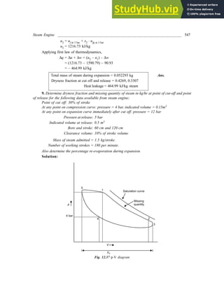


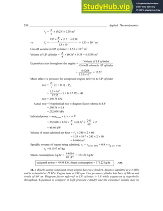


![Steam Engine _________________________________________________________________ 557
mep of HP referred to LP = 70.65 kPa
mep of LP = 62.96 kPa
Total output = 43.72 L kW where L is stroke length Ans.
15. During the trial of a single-cylinder double acting steam engine following is observed.
Duration of trial = 15 min, Bore = 25 cm, Stroke = 30 cm, Brake diameter = 1.5 m, Net
brake load = 300 N, Speed = 240 rpm, Steam pressure = 10 bar, Dryness fraction = 0.9, Cover end
mean effective pressure = 0.9 bar, Crank end mean effective pressure = 0.9 bar, Steam utilized =
15 kg. Condensate temperature = 45°C. Amount of water circulating = 450 kg/hr. Rise in cooling
water temperature = from 20°C to 30°C. Determine, (i) steam used per ihp. hr, (ii) mechanical
efficiency, (iii) brake thermal efficiency, (iv) heat balance sheet on one hour basis.
Solution:
From given data;
Average value of mean effective pressure =
1
2
(mepcover end + mep crank end)
mep = 0.9 bar
Steam consumption per hour =
15
15
´ 60 = 60 kg/hr
Indicated horse power =
mep L A N
´ ´ ´ ´
´
2
0 7457 60
.
,{as 1 HP = 0.7457kW}
=
0 10 0 30
4
0 240 2
60 0 7457
2 2
.9 . .25
.
´ ´ ´ ´ ´
´
( )
p
= 14.22 hp or 10.604 kJ/s or 38174.4 kJ/hr
Therefore, steam used per ihp. hr =
60
14.22
= 4.22 kg/ihp. hr
Steam used per ihp. hr = 4.22 kg/ihp. hr Ans.
Brake power can be obtained using the dynamometer data given i.e. brake load, brake drum
diameter etc.
Brake horse power = 3
2
60 0.7457 10
N T
π ⋅
× ×
=
2 240 300 0 75
60 0 7457 103
´ ´ ´ ´
´ ´
p .
.
Brake horse power = 7.58 hp or 5.65 kJ/s or 20340 kJ/hr
Mechanical efficiency =
Brakehorsepower
Indicated horse power
= 0.5331 or 53.31%
Heat available with steam/hr = 60 [hat 10 bar, 0.9 dry – hat 45°C]
= 60 [(762.81 + 0.9 ´ 2015.3) – (4.18 ´ 45)]
= 143308.8 kJ/hr](https://image.slidesharecdn.com/appliedthermodynamics3rdedition-230807154336-69e627e1/85/Applied-Thermodynamics-3rd-Edition-pdf-574-320.jpg)
![558 ________________________________________________________ Applied Thermodynamics
Brake thermal efficiency =
Heat equivalent of bhp
Heatavailablewithsteam / sec
=
7.58 ´ ´
0 7457 3600
143308 8
.
.
= 0.14199 or 14.19%
Heat carried away by circulating water in condenser
= 450 ´ 4.18 ´ [30 – 20]
= 18810 kJ/hr
Heat balance sheet on one hour basis
Input kJ % Output kJ %
Heat available 143308.8 100% bhp 20340 14.19
with steam/hr fhp(= ihp - bhp) 17834.4 12.44
Heat carried away by
circulating water 18810 13.13
Unaccounted losses 86324.4 60.24
(by difference)
Total 143308.8 100% Total 143308.8 100%
16. During trial of steam engine following observation are made; Bore:38 cm, Stroke 50 cm,
Piston rod diameter: 5 cm, Speed:150 rpm, Steam consumption: 36 kg/min, Brake load = 7kN at 2 m
brake diameter.
Area of indicator diagram at cover end: 28 cm2
Area of indicator diagram at crank end: 26cm2
Length of indicated diagram: 7 cm
Spring scale: 15 kPa/mm
Determine brake power, indicated power, mechanical efficiency, brake specific steam consumption
and indicated specific steam consumption.
Solution:
M.E.P.crank =
2600 15
70
×
= 557.14 kPa
M.E.P.cover =
2800 15
70
×
= 600 kPa
Indicated power at crank end, IPcrank = MEPcrank × L × Acrank × N
At crank end piston area will be reduced due to piston rod,
IPcrank = 557.14 × 50 × 10–2 ×
2 2 150
{(0.38) (0.05) }
4 60
π
− ×
IPcrank = 77.62 kW
Indicated power at cover end, IPcover = MEPcover × L × Acover × N
IPcover = 600 × 50 × 10–2 ×
2 150
(0.38)
4 60
π
× ×](https://image.slidesharecdn.com/appliedthermodynamics3rdedition-230807154336-69e627e1/85/Applied-Thermodynamics-3rd-Edition-pdf-575-320.jpg)
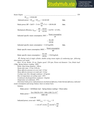
![Steam Engine _________________________________________________________________ 561
Engery loss to surroundings, Q4 = Qin – (Q1 + Q2 + Q3)
= 10175.64 – (507.6 + 3511.2 + 836) = 5320.84 kJ/min
Energy Balance sheet on per minute basis
Energy in, kJ/min Energy out, kJ/min
Energy supplied = 10175.64 Energy available at shaft = 507.6
Energy consumed by cooling water = 3511.2
Energy lost with condensate = 836
Energy loss to surroundings = 5320.84
Total: 10175.64, kJ/min Total: 10175.64 kJ/min
-:-4+15-
12.1 Classify steam engines.
12.2 Give a neat sketch of simple steam engine and explain its working.
12.3 Describe with sketches any five different parts of steam engines.
12.4 Why is it necessary to provide guides for a cross-head?
12.5 Describe the function of crank.
12.6 What is the eccentric? Explain its utility?
12.7 Describe the working of D-slide valve.
12.8 Describe hypothetical and actual indicator diagrams for a simple steam engine.
12.9 What are factors responsible for actual indicator diagram differing from hypothetical diagram?
12.10 Describe significance of diagram factor.
12.11 What do you understand by missing quantity of steam?
12.12 Why the cylinder of steam engine is generally steam jacketed?
12.13 What do you understand by compound steam engines?
12.14 Describe various types of compounding in steam engines and their relative merits and demerits.
12.15 Show the hypothetical and actual P-V diagram for compound steam engine having HP and LP
cylinders.
12.16 Discuss the relevance of mep referred to LP cylinder in compound steam engines.
12.17 Discuss different methods of governing of steam engines.
12.18 Explain Willan’s line.
12.19 What do you understand by unresisted expansion in reference to compound steam engines?
12.20 Discuss different types of governing of compound steam engines with p-V diagrams.
12.21 A single cylinder double acting steam engine is supplied with steam at 5 bar and steam is
exhausted at 0.34 bar. Cut-off occurs at one-third of stroke. The swept volume of cylinder is
0.05 m3
and diagram factor is 0.85. The engine delivers brake power of 37.5 kW at the speed of
120 rpm. Determine the mechanical efficiency of engine. [85%]
12.22 In a steam engine the steam is supplied at 20 bar, 340°C and is expanded adiabatically up to
1.5 bar after which there occurs instantaneous pressure drop at constant volume up to 0.07 bar.
Determine the work done per kg of steam supplied and the modified Rankine cycle efficiency.
[694.72 kJ, 23.5%]
12.23 Determine the indicated power output from a double acting single cylinder steam engine having
stroke of 30 cm and stroke to bore ratio of 1.3. The steam is admitted at 67.45 bar and the back](https://image.slidesharecdn.com/appliedthermodynamics3rdedition-230807154336-69e627e1/85/Applied-Thermodynamics-3rd-Edition-pdf-578-320.jpg)
![562 ________________________________________________________ Applied Thermodynamics
pressure is 1.3 bar with expansion ratio of 2.5. The engine runs at 210 rpm and the diagram factor
is 0.8. [27 kW]
12.24 A single cylinder double acting steam engine has steam being admitted at 10 bar, 0.96 dry and
exhausted at 0.5 bar. The expansion occurs up to 1.64 bar. Power output from engine is 60 hp at
210 rpm. The cylinder stroke volume is 0.021 m3
. Determine the diagram factor. [0.75]
12.25 A single cylinder double acting steam engine has bore of 25 cm and stroke to bore ratio of 1.2.
What shall be the indicated power output from engine if steam is admitted at 10.35 bar and
discharged at 0.34 bar. The diagram factor is 0.81 and cut off occurs at 50% of stroke.
[94.27 hp]
12.26 In a double acting steam engine the steam is supplied at 6.5 bar and 0.85 dry and exhausted at
0.28 bar. The engine runs with speed of 150 rpm. The diameter of piston is 500 mm and piston
rod has diameter of 64 mm. The expansion ratio at the front end and back end of piston are
10 and 8 respectively. Stroke length is 600 mm. Steam is being supplied at 6.8 kg per ihp. hr. Steam
leaving engine is condensed and the feed water at 35°C is sent back. Determine thermal efficiency
and total indicated horse power of engine. [19%, 159.6 hp]
12.27 A steam engine has throttle governing such that it develops 37.5 kW with steam consumption
of 1000 kg/hr. The steam consumption at no load is 125 kg/hr. Determine the steam consumption
for the indicated power developed being 25.8 kW. [750 kg/hr]
12.28 Determine the missing quantity of steam at cut-off, release and percentage reevaporation for the
double acting steam engine having following details.
Steam pressure at cut-off = 6 bar, the cut-off point is at distance of 38 cm from zero.
Steam pressure at release = 3 bar, the point of release is at distance of 8.3 cm from zero.
Steam pressure at beginning of compression = 1.05 bar, the point of start of compression is at distance
of 1.3 cm from zero.
Clearance length = 0.86 cm
Speed of engine = 150 rpm
Steam consumption = 270 kg/hr
Steam is supplied dry saturated.
Mean stroke volume = 7300 cm3
[0.005 kg, 0.003 kg, 32.4%]
12.29 In a two cylinder double acting compound steam engine the stroke in each cylinder is 50 cm and
the indicated power output is 220 kW at speed of 270 rpm. Steam is supplied at 12 bar and
exhausted at 0.28 bar. The total expansion ratio through the engine is 10 and the two cylinders
develop equal power. Neglecting clearance volume and assuming expansion to be complete in HP
cylinder and hyperbolic throughout determine the diameters of HP and LP cylinder.
[37.3 cm, 47.5 cm]
12.30 A double acting compound steam engine has HP and LP cylinder with steam being admitted at
17.25 bar and exhausted at 0.415 bar. Two cylinders have common stroke length with LP cylinder
having bore of 45 cm and stroke of 40 cm and HP cylinder bore is 28.5 cm. Engine runs at 270
rpm and the total expansion ratio is 9. The diagram factor of engine referred to LP cylinder is 0.78.
Considering hyperbolic expansion, zero clearance and each cylinder having equal initial piston
loads determine the intermediate pressure and indicated power of engine. [5.23 bar, 364.75 hp]
12.31 A double acting compound steam engine has stroke length of 40 cm for both HP and LP cylinders.
The bore of HP and LP cylinders are 30 cm and 60 cm respectively. The steam is supplied at
pressure of 13.8 bar and the back pressure is 0.28 bar. The cut-off in HP cylinder occurs at
1
3
rd of stroke. The engine develops brake power of 125 kW while running at 160 rpm. Considering
mechanical efficiency of 0.78 determine the actual and hypothetical mean effective pressures,
overall diagram factor. [2.66 bar, 3.73 bar, 0.7]](https://image.slidesharecdn.com/appliedthermodynamics3rdedition-230807154336-69e627e1/85/Applied-Thermodynamics-3rd-Edition-pdf-579-320.jpg)
![Steam Engine _________________________________________________________________ 563
12.32 Determine the overall diagram factor and the actual mean effective pressure of a triple expansion
engine having following details:
Steam admission pressure = 13.8 bar, Back pressure = 0.28 bar, Cut-off in HP = 60% of stroke
HP IP LP
Bore (cm) 30 45 75
Indicator Diagram area (mm2
) 1805 1875 2000
Indicator diagram length (mm) 104 105 103
Indicator constant (kg/mm2
/m) 40 16 5.35
[0.76, 3.18 bar]
12.33 A compound steam engine has following details;
No. of cylinders = 2, HP and LP.
HP cylinder piston area = 480 cm2 front and 450 cm2 back end.
LP cylinder piston area = 1920 cm2 front and 1890 cm2 back end.
Mean effective pressure of HP = 2.8 bar front and 2.67 back end.
Mean effective pressure of LP = 0.77 bar front and 0.84 back end.
Stroke length = 92 cm for both HP and LP.
Steam admission = 10.5 bar, dry saturated.
Temperature of hot well = 48°C
Speed of engine = 198 rpm
Steam consumption = 1225 kg per hour
Condenser circulating water requirement = 23400 kg/hr
Circulating water temperature rise = From 11°C to 36°C
Draw up a heat balance for engine on per minute basis and also determine thermal efficiency.
[Thermal efficiency = 17.7%]](https://image.slidesharecdn.com/appliedthermodynamics3rdedition-230807154336-69e627e1/85/Applied-Thermodynamics-3rd-Edition-pdf-580-320.jpg)
![564 ________________________________________________________ Applied Thermodynamics
13
Nozzles
13.1 INTRODUCTION
A nozzle is a flow passage of varying cross sectional area in which the velocity of fluid increases and
pressure drops in the direction of flow. Thus in nozzle the fluid enters the variable cross section area
duct with small velocity and high pressure and leaves it with high velocity and small pressure. During
flow through nozzle the enthalpy drops and heat drop in expansion is spent in increasing the velocity of
fluid. Similar to nozzle a duct with variable cross-section area will be called diffuser if the fluid gets
decelerated, causing a rise in pressure along the direction of flow. Nozzles are generally used in turbines,
jet engines, rockets, injectors, ejectors etc.
Fig. 13.1 General arrangement in nozzle and diffuser
Here in this chapter the one-dimensional analysis of nozzle has been considered.
Different types of nozzles, thermodynamic analysis and different phenomenon in nozzles are
discussed ahead.
Momentum transfer across the control volume may be accounted for as,
[Time rate of momentum transfer across the control volume] = m¢C
Newton’s law states that resultant force F acting on the control volume equals the difference
between the rates of momentum leaving and entering the control volume accompanying mass flow.
Momentum equation says;
F = m¢2 C2 – m¢1 C1
Since at steady state, m¢2 = m¢1 i.e. continuity equation being satisfied
F = m¢ (C2 – C1)
The resultant force F includes forces due to pressure acting at inlet and exit, forces acting on the
portion of the boundary through which there is no mass flow, and force due to gravity.](https://image.slidesharecdn.com/appliedthermodynamics3rdedition-230807154336-69e627e1/85/Applied-Thermodynamics-3rd-Edition-pdf-581-320.jpg)

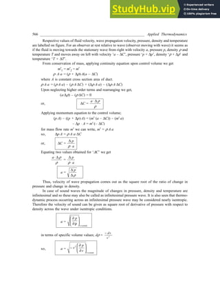


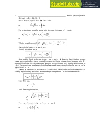

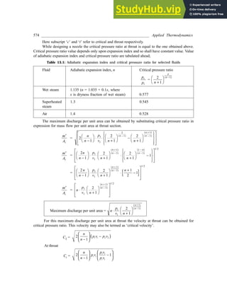


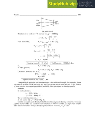


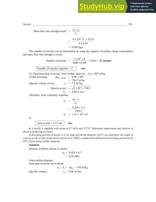


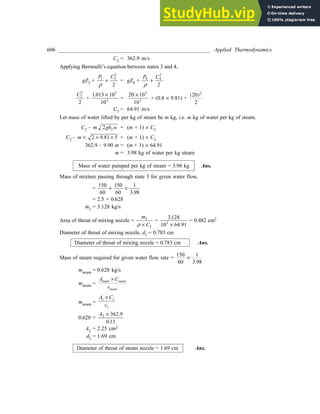


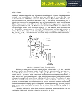


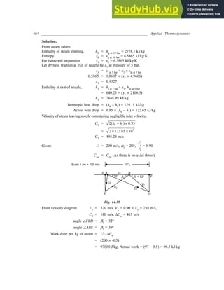


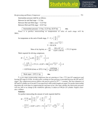


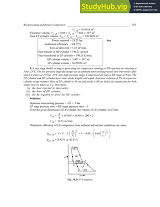


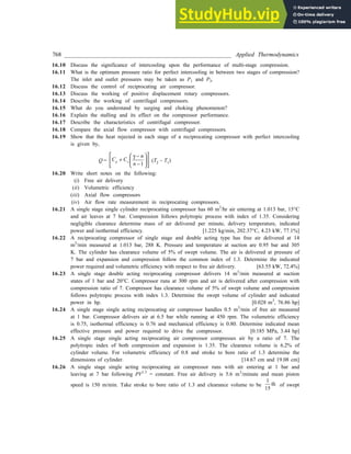


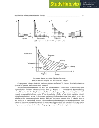


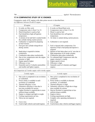


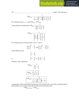


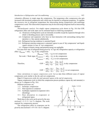


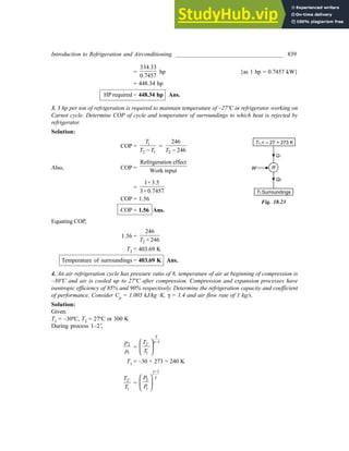


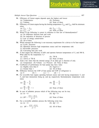


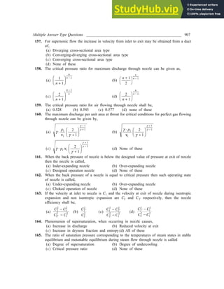


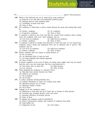
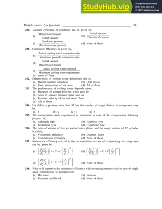


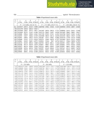


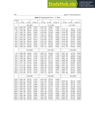


This document provides information about a textbook on engineering thermodynamics. It includes prefaces from the author for the third and first editions. The prefaces discuss the purpose and scope of the textbook, as well as acknowledgements. The document also provides a table of contents that lists the 18 chapters in the textbook, covering topics like the laws of thermodynamics, thermodynamic properties, cycles, and applications.