This document discusses Markov chains and their applications, including to genetics. It provides definitions and notations for stochastic processes and Markov chains. It then gives examples of using Markov chains to model genetics, including Mendelian inheritance where the probabilities of different genetic combinations in offspring can be represented through a transition matrix. The document concludes that Markov chains can be used to model the mixing of dominant and recessive genes across generations and calculate genetic probabilities from a mathematical perspective.

1. International Journal of Trend in Scientific Research and Development (IJTSRD)
Volume 3 Issue 5, August 2019 Available Online: www.ijtsrd.com e-ISSN: 2456 – 6470
@ IJTSRD | Unique Paper ID – IJTSRD27881 | Volume – 3 | Issue – 5 | July - August 2019 Page 2263
Applications on Markov Chain
Wai Mar Lwin1, Thinn Aung2, Khaing Khaing Wai3
1Faculty of Computing, 3Department of Information Support and Maintenance
2Department of Mathematics, Mandalay University, Myanmar
1,3University of Computer Studies, Mandalay, Myanmar
How to cite this paper: Wai Mar Lwin |
Thinn Aung | Khaing Khaing Wai
"Applications onMarkov Chain"Published
in International
Journal of Trend in
Scientific Research
and Development
(ijtsrd), ISSN: 2456-
6470, Volume-3 |
Issue-5, August
2019,pp.2263-2265,
https://doi.org/10.31142/ijtsrd27881
Copyright © 2019 by author(s) and
International Journal ofTrend inScientific
Research and Development Journal. This
is an Open Access article distributed
under the terms of
the Creative
Commons Attribution
License (CC BY 4.0)
(http://creativecommons.org/licenses/by
/4.0)
ABSTRACT
Markov chain is one of the techniques used in operations research with
possibilities view that managers in organizational decisionmaking (industrial
and commercial) use it. Markov processes arise in probability and statistics in
one of two ways. Markov process is a tool to predict that it can make logical
and accurate decisions about various aspects of management in the future.
KEYWORDS: Markov Chain, Probability, Stochastic
1. INTRODUCTION
Modern probability theory studies change process for which the knowledge of
previous outcomes influences predictions for future experiments. In principle,
when we observe a sequence of chance experiment, all of the past outcomes
could influence our predictions for the next experiment. For example, this
should be the case in predicting a student's grades on a sequence of exams in a
course. But to allow this much generality would make it very difficult to prove
general results.
In 1907, A.A. Markov began the study of an important new type of chance
process. In this process, the outcome of a given experiment can affect the
outcome of the next experiment.
2. SOME DEFINITIONS AND NOTATIONS
2.1 Stochastic Process
A stochastic process  Tt, tX is a collection of random variables.
The index t represents time and we refer Xt as the state of
the stochastic process at time t. The set T is called the index
set of the stochastic process. The index t is after interpreted
as time and as a result, as refer X(t) as the state of the
process at time.
It  .....2,1,,0T  , then the stochastic process is said to be
discrete-time process. It T is an interval of the real line, then
the stochastic process is said to be a continuous-time
process. For instance  .....2,1,0,n,Xn  is a discrete-
time process indexed by the non-negative integers; while
 0t,Xt  is a continuous-time stochastic processindexed
by the non-negative real numbers Let  ,.....2,1,0n,Xn 
be a discrete-time stochastic process. If Xn=i, then the
process is said to be state i at time n. A stochastic process
 ,.....2,1,0n,Xn  is called a Markov chain if
  ijnnnn PiXiXiXiXjXP   001111 ,,......,,|
This Equation may be interpreted as stating that; for a
Markovchain, theconditional distribution of anyfuturestate
Xn+1 given in the past states X0, X1, .....Xn-1 andthepresentstate
Xn, is independent of the past states and depends only on the
present state.
The value Pij denotes the probability that the Markov chain,
whenever in state i (the current state) moves next (one unit
of time later) into state j and is referred to as a one-step
transition probability. The transition probabilities are
collected into the one-step transition probability matrix. It is
denoted by P. This is,






2
12
02
1
11
01
0
10
00
iii P
P
P
P
P
P
P
P
P
P 
Since Probabilities are non-negative and since the process
must take a transition into some state, we have that
(i) 0ji,,0 ijP
(ii)
A state of a Markov chain is called absorbing if it is
impossible to leave it. A Markov chain is absorbing ifit has at
least one absorbing state and if from everystateitis possible
to go to an absorbing state (not necessarily in one step).
Markov chains have many applications as statistical models
of real-world processes.
2.2 Example (beauty and intelligence)
Albert Einstein was born on born March 14th, 1879 in
Germany. He died in April 18th, 1955. Marilyn Monroe was
an American actress and model. She was born on 1st June of
1926 in Los Angeles, United States. She died in August 5th,
1962.
IJTSRD27881

2. International Journal of Trend in Scientific Research and Development (IJTSRD) @ www.ijtsrd.com eISSN: 2456-6470
@ IJTSRD | Unique Paper ID – IJTSRD27881 | Volume – 3 | Issue – 5 | July - August 2019 Page 2264
At a dinner party, Einstein and Marilyn sat next to each
other. After a few flutes of champagne, she cooked in his
attentive ear: "I want to have your child. With my looks and
your brains, it will be a perfect child!" Einstein replied: "But
what if it has my looks and your brains?"
According to this quote, we can constructMarkov Model.For
example:
The child will be perfect child because of the combination of
beauty and intelligence or the child will be ugly and
ignoramus. For more details of genus model I discussed in
next example.
2.3 Example (Simple Mendelian inheritance)
A certain trait is determined by a specific pair of genes, each
of which may be two types, say G and g.
One individual may have:
 GG combination (dominant)
 Gg or gG, considered equivalent genetically (hybrid)
 gg combination (recessive)
In sexual reproduction, offspring inherit one geneofthepair
from each parent.
2.3.1 Basic assumption of Mendelian genetics
Genes inherited from each parent are selected at random,
independently of each other. This determines probability of
occurrence of each type of offspring. The offspring
 of two GG parents must be GG,
 of two gg parents must be gg,
 of one GG and one gg parent must be Gg,
 Other cases must be examined in more detail.
2.3.2 Gg and Gg parents
Offspring has probability

1
4
of being GG

1
2
of being Gg

1
4
of being gg
2.3.3 GG and Gg parents
Offspring has probability

1
2
of being GG

1
2
of being Gg
2.3.4 gg and Gg parents
Offspring has probability

1
2
of being Gg

1
2
of being gg
Let pi(n + 1) be the probability that state Si , 1  i  r , occurs
on(n + 1)th repetition of the experiment.
There are r ways to be in state Si at step n + 1:
1. Step n is S1. Probability of getting S1 on nth step is p1(n),
and Probability of having Si after S1 is p1i. Therefore, by
multiplication Principle, P (Si |S1) = p1ip1 (n).
2. We get S2 on step n and Si on step (n + 1).
Then P (Si |S2) =p2ip2 (n).
r. Probability of occurrence of Si at step n + 1 if Sr at step n is
P (Si |Sr ) = pripr(n).
Therefore, pi (n + 1) is sum of all these,
pi (n + 1) = P(Si |S1) + · + P(Si |Sr )
= p1ip1 (n) + · + pripr(n)
2.3.5 General case
Let pi(n) be the probability that the state Si will occur on the
nth repetition of the experiment, 1 i  r .
Since one the states Si must occur on the nth repetition,
p1(n) + p2(n) + · · · + pr(n) = 1.
Therefore,
p1(n + 1) = p11p1(n) + p21p2(n) + · · · + pr1pr(n)
...........

3. International Journal of Trend in Scientific Research and Development (IJTSRD) @ www.ijtsrd.com eISSN: 2456-6470
@ IJTSRD | Unique Paper ID – IJTSRD27881 | Volume – 3 | Issue – 5 | July - August 2019 Page 2265
pk(n + 1) = p1kp1(n) + p2kp2(n) + · · · + prkpr(n) (1)
............
pr(n + 1) = p1rp1(n) + p2rp2(n) + · · · + prrpr(n)
In matrix form
p(n + 1) = p(n)P, n = 1, 2, 3, . . . (2)
Where p(n) = {p1(n), p2(n), . . . , pr(n)} is a (row) probability
vector and P = (pij ) is a r × r transition matrix,
11 12 1
21 22 2
1 2
.....
.....
.... ..... ..... ....
.....
r
r
r r rr
p p p
p p p
p
p p p
 
 
 
 
  
 
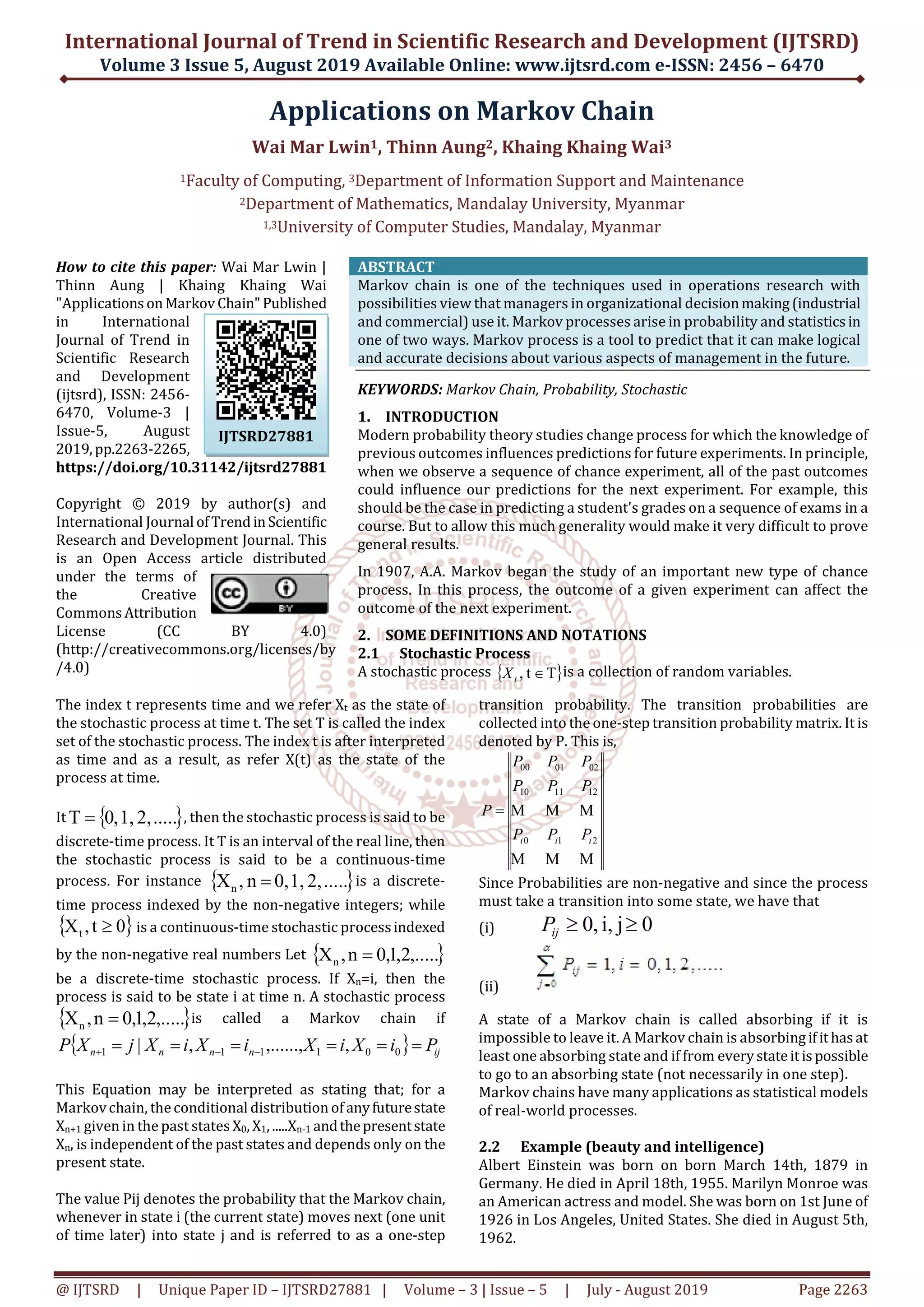
For our genetic model..
Consider a process of continued mating.
 Start with an individual of known or unknown genetic
character and mate it with a hybrid.
 Assume that there is at least oneoffspring;chooseoneof
them at random and mate it with a hybrid.
 Repeat this process through a number of generations.
The genetic type of the chosen offspring in successive
generations can be represented by a Markov chain, with
states GG, Gg and gg.
So there are 3 possible states S1 = GG, S2 =Gg and S3 = gg.
So, what we have is
[p1(n + 1), . . . , pr (n + 1)] =
[p1(n ), . . . , pr (n )]
11 12 1
21 22 2
1 2
....
....
.... .... .... ....
....
r
r
r r rr
p p p
p p p
p p p
 
 
 
 
  
 
It is easy to check that this gives the same expression as (1)
We have
GG Gg gg
GG 0.5 0.5
Gg 0.25 0.5
gg 0 0.5
The transition probabilities are
0.5 0.5 0
0.25 0.5 0.25
0 0.5 0.5
p
 
 
  
 
 
The two step transition matrix is
(2)
0.5 0.5 0 0.5 0.5 0 0.375 0.5 0.125
0.25 0.5 0.25 0.25 0.5 0.25 0.25 0.5 0.25
0 0.5 0.5 0 0.5 0.5 0.125 0.5 0.375
p
    
    
     
    
    
This result showed the fact thatwhenthedominantgene and
the recessive gene mixed the different types, the dominant
gene reappeared in second generation and later.
3. CONCLUSION
This paper aims to present the genetic science from the
mathematical point of view. To do research more from this
paper, a new, well-qualified genetic one can be produced in
combination with two existing genetics. In accordance with
calculating or speculating the genetic probability from the
mathematical aspect, it may be the logical impossibility in
real world.
REFERENCES
[1] A. M. Natarajan & A. Tamilarasi , Probability Random
Process & Queuing Theory, New Age International (p)
Ltd, Publishers, New Delhi ,2003.
[2] S. M. Ross, Stochastic Process, John Wiley & sons, New
York, 1983.
[3] S. M. Ross, Introduction to Probability Models, (Tenth
Edition), Academic Press, New York, 2010.