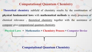
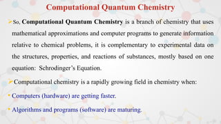
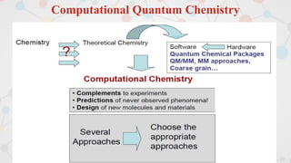
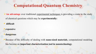
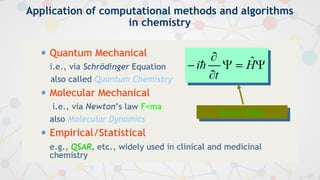
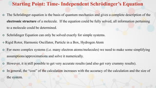
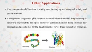
Presented By
Dr. Khulood Obaid Kzar Al-Masoodi
University of Kerbala … Faculty of Science … Department of Chemistry
20-21.4.020-2021
Applications of Computational Quantum Chemistry
Computational Quantum Chemistry
Theoretical chemistry subfield of chemistry results by the combination of
physical fundamental laws with mathematical methods to study processes of
chemical relevance , theoretical chemistry together with the assistance of
computer give computational quantum chemistry.
Physical Laws + Mathematics + Chemistry Process + Computer Device
Computational Quantum Chemistry
So, Computational Quantum Chemistry is a branch of chemistry that uses
mathematical approximations and computer programs to generate information
relative to chemical problems, it is complementary to experimental data on
the structures, properties, and reactions of substances, mostly based on one
equation: Schrodinger’s Equation.
Computational chemistry is a rapidly growing field in chemistry when:
• Computers (hardware) are getting faster.
• Algorithms and programs (software) are maturing.
Computational Quantum Chemistry
An advantage over traditional experimental techniques is providing a route to the study
of chemical questions which may be experimentally:
 difficult
 expensive
 dangerous
 Because of the difficulty of dealing with nano-sized materials, computational modeling
has become an important characterization tool in nanotechnology.
Application of computational methods and algorithms
in chemistry
Starting Point: Time- Independent Schrödinger’s Equation
 The Schrödinger equation is the basis of quantum mechanics and gives a complete description of the
electronic structure of a molecule. If the equation could be fully solved, all information pertaining
to a molecule could be determined.
 Schrödinger Equation can only be solved exactly for simple systems.
 Rigid Rotor, Harmonic Oscillator, Particle in a Box, Hydrogen Atom
 For more complex systems (i.e. many electron atoms/molecules) we need to make some simplifying
assumptions/approximations and solve it numerically.
 However, it is still possible to get very accurate results (and also get very crummy results).
 In general, the “cost” of the calculation increases with the accuracy of the calculation and the size of
the system.
Starting Point: Time- Independent Schrödinger’s Equation
Development of the Schrödinger equation from other fundamental laws of
physics.
Time- Independent Schrödinger’s Equation
The Main Three Approximations
1. Born-Oppenheimer Approximation
Electrons act separately of nuclei, electron and nuclear coordinates are independent of
each other, and thus simplifying the Schrödinger equation
Independent particle approximation.
1. Electrons experience the ‘field’ of all other electrons as a group, not
individually
Give birth to the concept of “orbital”, e.g., AO, MO, etc.
1. LCAO-MO approximation
Molecular orbitals (MO) can be constructed as linear combinations of
atom orbitals, to form Slater determinants.
Born-Oppenheimer Approximation
• The wave-function of the many-electron molecule is a function of electron and nuclear
coordinates: (R,r) (R=nuclear coords, r=electron coords).
• The motions of the electrons and nuclei are coupled.
• However, the nuclei are much heavier than the electrons
– mp ≈ 2000 me
• And consequently nuclei move much more slowly than do the electrons (E=1/2mv2). To the
electrons the nuclei appear fixed.
• Born-Oppenheimer Approximation: to a high degree of accuracy we can separate electron and
nuclear motion:
(R,r)= el(r;R) N(R)
Types of Calculations
 There are three basic types of calculations.
From these calculations, other information can be determined.
• Single-Point Energy: predict stability, reaction mechanisms
• Geometry Optimization: predict shape
• Frequency: predict spectra
Computational Models
 A model is a system of equations, or computations used to determine the
energetics of a molecule
 Different models use different approximations (or levels of theory) to
produce results of varying levels of accuracy.
 There is a trade off between accuracy and computational time.
 There are two main types of models; those that use Schrödinger's
equation (or simplifications of it) and those that do not.
Computational Models
 Types of Models
(Listed in order from most to least accurate)
 Ab initio
• uses Schrödinger's equation, but with approximations
 Semi Empirical
•uses experimental parameters and extensive simplifications of
Schrödinger's equation
 Molecular Mechanics
•does not use Schrödinger's equation
Ab Initio
 Ab initio translated from Latin means “from first principles.” This refers to the
fact that no experimental data is used and computations are based on quantum
mechanics.
 Different Levels of Ab Initio Calculations
 Hartree-Fock (HF)
•The simplest ab initio calculation
•The major disadvantage of HF calculations is that electron correlation is
not taken into consideration.
 The Møller-Plesset Perturbation Theory (MP)
 Density Functional Theory (DFT)
 Configuration Interaction (CI) Take into consideration
electron correlation
Ab Initio
 Approximations used in some ab initio calculations
 Central field approximation: integrates the electron-electron repulsion
term, giving an average effect instead of an explicit energy
 Linear combination of atomic orbitals (LCAO): is used to describe the
wave function and these functions are then combined into a
determinant. This allows the equation to show that an electron was put
in an orbital, but the electron cannot be specified.
Density Functional Theory
Considered an ab initio method, but different from other ab initio methods because the
wavefunction is not used to describe a molecule, instead the electron density is used.
Three types of DFT calculations exist:
• local density approximation (LDA) – fastest method, gives less accurate geometry,
but provides good band structures.
• gradient corrected - gives more accurate geometries.
• hybrids (which are a combination of DFT and HF methods) - give more accurate
geometries.
Self-Consistent-Field (SCF)
1.Choose start coefficients for MO’s.
2.Construct Fock Matrix with coefficients.
3.Solve Hartree-Fock-Roothaan equations.
4.Repeat 2 and 3 until ingoing and outgoing coefficients are the same.





  S
F 
  i
i
i c
c
Semi Empirical
 Semi empirical methods use experimental data to parameterize equations
 Like the ab initio methods, a Hamiltonian and wave function are used
 much of the equation is approximated or eliminated
 Less accurate than ab initio methods but also much faster
 The equations are parameterized to reproduce specific results, usually the geometry
and heat of formation, but these methods can be used to find other data.
Molecular Mechanics
 Simplest type of calculation
 Used when systems are very large and approaches that are more accurate become to costly (in time
and memory)
 Does not use any quantum mechanics instead uses parameters derived from experimental or ab initio
data
 Uses information like bond stretching, bond bending, torsions, electrostatic interactions, van der
Waals forces and hydrogen bonding to predict the energetics of a system
 The energy associated with a certain type of bond is applied throughout the molecule. This leads to
a great simplification of the equation
 It should be clarified that the energies obtained from molecular mechanics do not have any physical
meaning, but instead describe the difference between varying conformations (type of isomer).
Molecular mechanics can supply results in heat of formation if the zero of energy is taken into account.
Size vs Accuracy
Basis Sets
 In chemistry a basis set is a group of mathematical functions used to describe the shape
of the orbitals in a molecule, each basis set is a different group of constants used in the
wavefunction of the Schrödinger equation.
 The accuracy of a calculation is dependent on both the model and the type of basis set
applied to it.
 Once again there is a trade off between accuracy and time. Larger basis sets will
describe the orbitals more accurately but take longer to solve.
 General expression for a basis function = N * e(- * r)
 where: N is the normalization constant,  is the orbital exponent, and r is the radius
of the orbital in angstroms.
Examples of Basis Sets
 STO-3G basis set - simplest basis set, uses the minimal number of functions to describe each atom in the
molecule
 for nanotube systems this means hydrogen is described by one function (for the 1s orbital), while carbon
is described by five functions (1s, 2s, 2px, 2py and 2pz).
 Split valence basis sets use two functions to describe different sizes of the same orbitals.
 For example with a split valence basis set H would be described by two functions while C would be
described by 10 functions.
 6-31G or 6-311G (which uses three functions for each orbital, a triple split valence set).
 Polarized basis sets - improve accuracy by allowing the shape of orbitals to change by adding orbitals
beyond that which is necessary for an atom
 6-31G(d) (also known as the 6-31G*) - adds a d function to carbon atoms
• “The underlying physical laws necessary for the mathematical
theory of a large part of physics and the whole of chemistry are
thus completely known, and the difficulty is only that the exact
application of these laws leads to equations much too
complicated to be soluble.”
• Caution! : Different choices of methods and basis sets can yield a
large variation in results.
Thank You For Your Attention
Some of the almost limitless properties that can be calculated with
computational chemistry are:
– Geometry Optimization
– Stability and Reaction Mechanism
– Transition-state structures
– Dipole moments and polarizabilities
– Electron and Hole Density Distribution Maps
– Vibrational frequencies, IR and Raman Spectra
– NMR spectra
– Electronic excitations and UV spectra
– Thermochemical data
Geometry Optimization
• The objective of geometry optimization is to find an atomic arrangement which
makes the molecule most stable. Molecules are most stable when their energy is
low.
Stability and Reaction Mechanism
Dipole moments and polarizabilities
Electron and Hole Density Distribution Maps
Vibrational frequencies
Electronic excitations and UV spectra
Other Applications
• Also, computational Chemistry is widely used in studying the biological activity and
protein structure.
• Among one of the greatest gifts computer science had contributed to drug discovery is
the ability to predict the biological activity of compounds and in doing so drives new
prospects and possibilities for the development of novel drugs with robust properties.
Thank You For Your Attention

Applications of Computational Quantum Chemistry

  • 1.
    Presented By Dr. KhuloodObaid Kzar Al-Masoodi University of Kerbala … Faculty of Science … Department of Chemistry 20-21.4.020-2021 Applications of Computational Quantum Chemistry
  • 3.
    Computational Quantum Chemistry Theoreticalchemistry subfield of chemistry results by the combination of physical fundamental laws with mathematical methods to study processes of chemical relevance , theoretical chemistry together with the assistance of computer give computational quantum chemistry. Physical Laws + Mathematics + Chemistry Process + Computer Device Computational Quantum Chemistry
  • 4.
    Computational Quantum Chemistry So,Computational Quantum Chemistry is a branch of chemistry that uses mathematical approximations and computer programs to generate information relative to chemical problems, it is complementary to experimental data on the structures, properties, and reactions of substances, mostly based on one equation: Schrodinger’s Equation. Computational chemistry is a rapidly growing field in chemistry when: • Computers (hardware) are getting faster. • Algorithms and programs (software) are maturing.
  • 5.
  • 6.
    Computational Quantum Chemistry Anadvantage over traditional experimental techniques is providing a route to the study of chemical questions which may be experimentally:  difficult  expensive  dangerous  Because of the difficulty of dealing with nano-sized materials, computational modeling has become an important characterization tool in nanotechnology.
  • 7.
    Application of computationalmethods and algorithms in chemistry
  • 8.
    Starting Point: Time-Independent Schrödinger’s Equation  The Schrödinger equation is the basis of quantum mechanics and gives a complete description of the electronic structure of a molecule. If the equation could be fully solved, all information pertaining to a molecule could be determined.  Schrödinger Equation can only be solved exactly for simple systems.  Rigid Rotor, Harmonic Oscillator, Particle in a Box, Hydrogen Atom  For more complex systems (i.e. many electron atoms/molecules) we need to make some simplifying assumptions/approximations and solve it numerically.  However, it is still possible to get very accurate results (and also get very crummy results).  In general, the “cost” of the calculation increases with the accuracy of the calculation and the size of the system.
  • 9.
    Starting Point: Time-Independent Schrödinger’s Equation Development of the Schrödinger equation from other fundamental laws of physics.
  • 10.
  • 11.
    The Main ThreeApproximations 1. Born-Oppenheimer Approximation Electrons act separately of nuclei, electron and nuclear coordinates are independent of each other, and thus simplifying the Schrödinger equation Independent particle approximation. 1. Electrons experience the ‘field’ of all other electrons as a group, not individually Give birth to the concept of “orbital”, e.g., AO, MO, etc. 1. LCAO-MO approximation Molecular orbitals (MO) can be constructed as linear combinations of atom orbitals, to form Slater determinants.
  • 12.
    Born-Oppenheimer Approximation • Thewave-function of the many-electron molecule is a function of electron and nuclear coordinates: (R,r) (R=nuclear coords, r=electron coords). • The motions of the electrons and nuclei are coupled. • However, the nuclei are much heavier than the electrons – mp ≈ 2000 me • And consequently nuclei move much more slowly than do the electrons (E=1/2mv2). To the electrons the nuclei appear fixed. • Born-Oppenheimer Approximation: to a high degree of accuracy we can separate electron and nuclear motion: (R,r)= el(r;R) N(R)
  • 13.
    Types of Calculations There are three basic types of calculations. From these calculations, other information can be determined. • Single-Point Energy: predict stability, reaction mechanisms • Geometry Optimization: predict shape • Frequency: predict spectra
  • 14.
    Computational Models  Amodel is a system of equations, or computations used to determine the energetics of a molecule  Different models use different approximations (or levels of theory) to produce results of varying levels of accuracy.  There is a trade off between accuracy and computational time.  There are two main types of models; those that use Schrödinger's equation (or simplifications of it) and those that do not.
  • 15.
    Computational Models  Typesof Models (Listed in order from most to least accurate)  Ab initio • uses Schrödinger's equation, but with approximations  Semi Empirical •uses experimental parameters and extensive simplifications of Schrödinger's equation  Molecular Mechanics •does not use Schrödinger's equation
  • 16.
    Ab Initio  Abinitio translated from Latin means “from first principles.” This refers to the fact that no experimental data is used and computations are based on quantum mechanics.  Different Levels of Ab Initio Calculations  Hartree-Fock (HF) •The simplest ab initio calculation •The major disadvantage of HF calculations is that electron correlation is not taken into consideration.  The Møller-Plesset Perturbation Theory (MP)  Density Functional Theory (DFT)  Configuration Interaction (CI) Take into consideration electron correlation
  • 17.
    Ab Initio  Approximationsused in some ab initio calculations  Central field approximation: integrates the electron-electron repulsion term, giving an average effect instead of an explicit energy  Linear combination of atomic orbitals (LCAO): is used to describe the wave function and these functions are then combined into a determinant. This allows the equation to show that an electron was put in an orbital, but the electron cannot be specified.
  • 18.
    Density Functional Theory Consideredan ab initio method, but different from other ab initio methods because the wavefunction is not used to describe a molecule, instead the electron density is used. Three types of DFT calculations exist: • local density approximation (LDA) – fastest method, gives less accurate geometry, but provides good band structures. • gradient corrected - gives more accurate geometries. • hybrids (which are a combination of DFT and HF methods) - give more accurate geometries.
  • 20.
    Self-Consistent-Field (SCF) 1.Choose startcoefficients for MO’s. 2.Construct Fock Matrix with coefficients. 3.Solve Hartree-Fock-Roothaan equations. 4.Repeat 2 and 3 until ingoing and outgoing coefficients are the same.        S F    i i i c c
  • 21.
    Semi Empirical  Semiempirical methods use experimental data to parameterize equations  Like the ab initio methods, a Hamiltonian and wave function are used  much of the equation is approximated or eliminated  Less accurate than ab initio methods but also much faster  The equations are parameterized to reproduce specific results, usually the geometry and heat of formation, but these methods can be used to find other data.
  • 22.
    Molecular Mechanics  Simplesttype of calculation  Used when systems are very large and approaches that are more accurate become to costly (in time and memory)  Does not use any quantum mechanics instead uses parameters derived from experimental or ab initio data  Uses information like bond stretching, bond bending, torsions, electrostatic interactions, van der Waals forces and hydrogen bonding to predict the energetics of a system  The energy associated with a certain type of bond is applied throughout the molecule. This leads to a great simplification of the equation  It should be clarified that the energies obtained from molecular mechanics do not have any physical meaning, but instead describe the difference between varying conformations (type of isomer). Molecular mechanics can supply results in heat of formation if the zero of energy is taken into account.
  • 23.
  • 24.
    Basis Sets  Inchemistry a basis set is a group of mathematical functions used to describe the shape of the orbitals in a molecule, each basis set is a different group of constants used in the wavefunction of the Schrödinger equation.  The accuracy of a calculation is dependent on both the model and the type of basis set applied to it.  Once again there is a trade off between accuracy and time. Larger basis sets will describe the orbitals more accurately but take longer to solve.  General expression for a basis function = N * e(- * r)  where: N is the normalization constant,  is the orbital exponent, and r is the radius of the orbital in angstroms.
  • 25.
    Examples of BasisSets  STO-3G basis set - simplest basis set, uses the minimal number of functions to describe each atom in the molecule  for nanotube systems this means hydrogen is described by one function (for the 1s orbital), while carbon is described by five functions (1s, 2s, 2px, 2py and 2pz).  Split valence basis sets use two functions to describe different sizes of the same orbitals.  For example with a split valence basis set H would be described by two functions while C would be described by 10 functions.  6-31G or 6-311G (which uses three functions for each orbital, a triple split valence set).  Polarized basis sets - improve accuracy by allowing the shape of orbitals to change by adding orbitals beyond that which is necessary for an atom  6-31G(d) (also known as the 6-31G*) - adds a d function to carbon atoms
  • 26.
    • “The underlyingphysical laws necessary for the mathematical theory of a large part of physics and the whole of chemistry are thus completely known, and the difficulty is only that the exact application of these laws leads to equations much too complicated to be soluble.” • Caution! : Different choices of methods and basis sets can yield a large variation in results.
  • 27.
    Thank You ForYour Attention
  • 29.
    Some of thealmost limitless properties that can be calculated with computational chemistry are: – Geometry Optimization – Stability and Reaction Mechanism – Transition-state structures – Dipole moments and polarizabilities – Electron and Hole Density Distribution Maps – Vibrational frequencies, IR and Raman Spectra – NMR spectra – Electronic excitations and UV spectra – Thermochemical data
  • 30.
    Geometry Optimization • Theobjective of geometry optimization is to find an atomic arrangement which makes the molecule most stable. Molecules are most stable when their energy is low.
  • 31.
  • 32.
    Dipole moments andpolarizabilities
  • 33.
    Dipole moments andpolarizabilities
  • 34.
    Electron and HoleDensity Distribution Maps
  • 35.
  • 36.
  • 37.
  • 38.
    Other Applications • Also,computational Chemistry is widely used in studying the biological activity and protein structure. • Among one of the greatest gifts computer science had contributed to drug discovery is the ability to predict the biological activity of compounds and in doing so drives new prospects and possibilities for the development of novel drugs with robust properties.
  • 39.
    Thank You ForYour Attention