

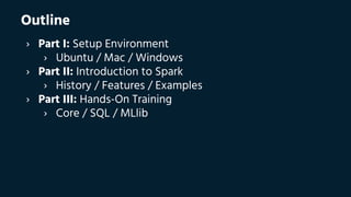


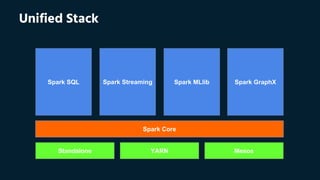
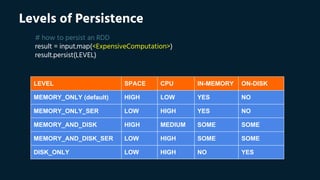
![Validate Setup
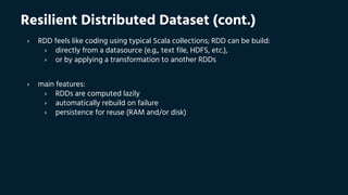
# import required libraries
from pyspark import SparkConf, SparkContext
# create spark context
sc = SparkContext(conf=(SparkConf().setMaster("local[*]")))
# print spark context
print(sc)
# print spark configuration
print(sc._conf.getAll())](https://image.slidesharecdn.com/euangeloslinardos20160402apachesparkworkshop-160409103945/85/Apache-Spark-Workshop-Apr-2016-Euangelos-Linardos-7-320.jpg)

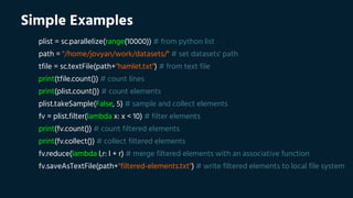

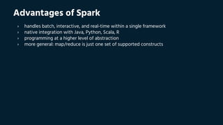

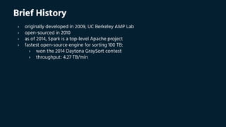
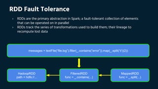


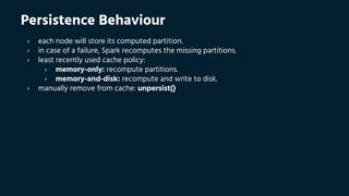
![master description
local
run Spark locally with one worker thread (i.
e. no parallelism at all)
local[*]
run Spark locally with as many worker
threads as logical cores on your machine
spark://HOST:PORT
connect to the given Spark standalone
cluster master (port 7077 by default)
mesos://HOST:PORT
connect to the given Mesos cluster
(port 5050 by default)
yarn
connect to a YARN cluster in client or
cluster mode (YARN_CONF_DIR variable)
The Spark Master
› the master parameter for a SparkContext determines which cluster to use:](https://image.slidesharecdn.com/euangeloslinardos20160402apachesparkworkshop-160409103945/85/Apache-Spark-Workshop-Apr-2016-Euangelos-Linardos-28-320.jpg)


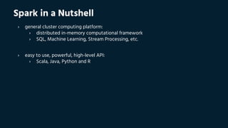
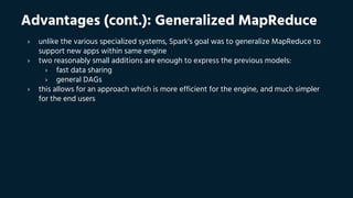
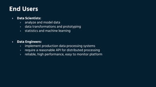
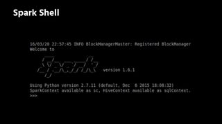
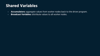
![Word Count (cont.)
# calculate word frequencies
counts = (tfile.
flatMap(lambda x: x.split(' ')).
filter(lambda x: len(x) > 0).
map(lambda x: (x, 1)).
reduceByKey(lambda l,r: l + r).
sortBy(lambda x: x[1], ascending=False))
# print (word,count) sample
print(counts.take(5))](https://image.slidesharecdn.com/euangeloslinardos20160402apachesparkworkshop-160409103945/85/Apache-Spark-Workshop-Apr-2016-Euangelos-Linardos-31-320.jpg)
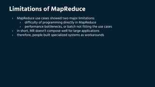
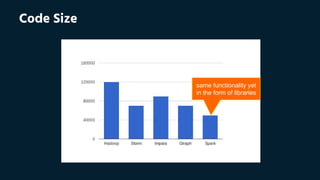
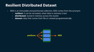
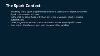
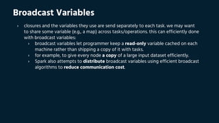
![Mining Logs
# base RDD
logRDD = sc.textFile(path+"logs.txt")
# transformed RDDs
filteredRDD = logRDD.filter(lambda x: u' "GET ' in x)
splittedRDD = filteredRDD.map(lambda x: x.split(u' "GET ')).map(lambda x: x[1])
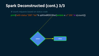
# count requests based on status code
print('with status “200”: %d' % splittedRDD.filter(lambda x: u'" 200 ' in x).count())
print('without status “200”: %d' % splittedRDD.filter(lambda x: u'" 200 ' not in x).count())](https://image.slidesharecdn.com/euangeloslinardos20160402apachesparkworkshop-160409103945/85/Apache-Spark-Workshop-Apr-2016-Euangelos-Linardos-32-320.jpg)
![Spark Deconstructed (cont.) 2/3
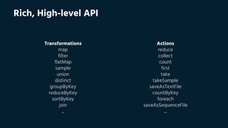
# transformed RDDs
filteredRDD = logRDD.filter(lambda x: u' "GET ' in x)
splittedRDD = filteredRDD.map(lambda x: x.split(u' "GET ')).map(lambda x: x[1])
transform
ation(s)
RDD](https://image.slidesharecdn.com/euangeloslinardos20160402apachesparkworkshop-160409103945/85/Apache-Spark-Workshop-Apr-2016-Euangelos-Linardos-35-320.jpg)
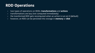
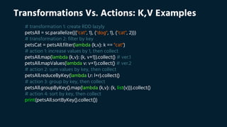
![Transformations Vs. Actions: Join Examples
# transformation 1: RDD[(date, user, clicks)]
clk = sc.textFile(path+"clk.tsv").map(lambda x: x.split("t"))
# transformation 2: RDD[(date, user, id, lat, lon)]
reg = sc.textFile(path+"reg.tsv").map(lambda x: x.split("t"))
# transformation 3: RDD[(user, (date, clicks))]
clk_reordered = clk.map(lambda (date, user, clicks): (user, (date, clicks)))
# transformation 4: RDD[(user, (date, id, lat, lon))]
reg_reordered = reg.map(lambda (date, user, id, lat, lon): (user, (date, id, lat, lon)))
# transformation 5: RDD[(user, ((date, clicks), (date, id, lat, lon)))]
joined = clk_reordered.join(reg_reordered)
print(joined.count()) # action 1: print total number of successful joins
print(joined.first()) # action 2: print first element of newly-joined RDD](https://image.slidesharecdn.com/euangeloslinardos20160402apachesparkworkshop-160409103945/85/Apache-Spark-Workshop-Apr-2016-Euangelos-Linardos-43-320.jpg)
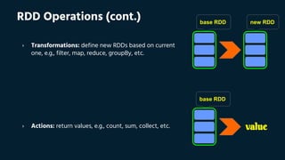
![Lineage Graph
# calculate word frequencies
counts = (sc.textFile(path+"hamlet.txt"). # MappedRDD[1], HadoopRDD[0]
flatMap(lambda x: x.split(' ')). # FlatMappedRDD[2]
map(lambda x: (x, 1)). # MappedRDD[3]
reduceByKey(lambda l,r: l + r)) # ShuffledRDD[4]
# print lineage graph representation
print(counts.toDebugString())
[0] [1] [2] [3] [4]
HadoopRDD MappedRDD FlatMappedRDD MappedRDD ShuffledRDD](https://image.slidesharecdn.com/euangeloslinardos20160402apachesparkworkshop-160409103945/85/Apache-Spark-Workshop-Apr-2016-Euangelos-Linardos-46-320.jpg)
![Lineage Graph (cont.)
# calculate word frequencies
counts = (sc.textFile(path+"hamlet.txt"). # MappedRDD[1], HadoopRDD[0]
flatMap(lambda x: x.split(' ')). # FlatMappedRDD[2]
map(lambda x: (x, 1)). # MappedRDD[3]
reduceByKey(lambda l,r: l + r)) # ShuffledRDD[4]
# print lineage graph representation
print(counts.toDebugString())
[0] [1] [2] [3] [4]
HadoopRDD MappedRDD FlatMappedRDD MappedRDD ShuffledRDD
[0] [1] [2] [3] [4]](https://image.slidesharecdn.com/euangeloslinardos20160402apachesparkworkshop-160409103945/85/Apache-Spark-Workshop-Apr-2016-Euangelos-Linardos-47-320.jpg)
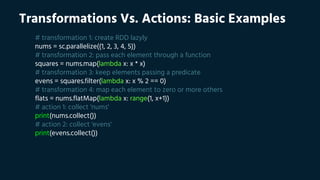
![Execution Plan
# calculate word frequencies
counts = (sc.textFile(path+"hamlet.txt"). # MappedRDD[1], HadoopRDD[0]
flatMap(lambda x: x.split(' ')). # FlatMappedRDD[2]
map(lambda x: (x, 1)). # MappedRDD[3]
reduceByKey(lambda l,r: l + r)) # ShuffledRDD[4]
# print lineage graph representation
print(counts.toDebugString())
[0] [1] [2] [3] [4]
HadoopRDD MappedRDD FlatMappedRDD MappedRDD ShuffledRDD
[0] [1] [2] [3] [4]
Stage 1 Stage 2](https://image.slidesharecdn.com/euangeloslinardos20160402apachesparkworkshop-160409103945/85/Apache-Spark-Workshop-Apr-2016-Euangelos-Linardos-48-320.jpg)

![Example Without Broadcast Variables
# dict(user: (date, id, lat, lon))
regDict = dict(reg_reordered.collect())
# CAUTION: regDict is sent along with every task!
joined = clk_reordered.
map(lambda (user, (date, clicks)): (user, ((date, clicks), regDict[user])))
# let's have a look on the output, transformed dataset
print(joined.first())
print(joined.count())](https://image.slidesharecdn.com/euangeloslinardos20160402apachesparkworkshop-160409103945/85/Apache-Spark-Workshop-Apr-2016-Euangelos-Linardos-55-320.jpg)
![Example With Broadcast Variables
# dict(user: (date, id, lat, lon))
regDict = dict(reg_reordered.collect())
bcDict = sc.broadcast(regDict)
# bcDict is a read-only variable, cached on each machine
joined = clk_reordered.
map(lambda (user, (date, clicks)): (user, ((date, clicks), bcDict.value[user])))
# let's have a look on the output, transformed dataset
print(joined.first())
print(joined.count())](https://image.slidesharecdn.com/euangeloslinardos20160402apachesparkworkshop-160409103945/85/Apache-Spark-Workshop-Apr-2016-Euangelos-Linardos-56-320.jpg)


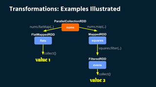
![Basic Summary Statistics
# define auxiliary functions
def computeStats(column):
return [round(column.count(),0),
round(column.sum(),3),
round(column.max(),3),
round(column.min(),3),
round(column.mean(),3),
round(computeMedian(column),3),
round(column.stdev(),3),
round(column.variance(),3)]](https://image.slidesharecdn.com/euangeloslinardos20160402apachesparkworkshop-160409103945/85/Apache-Spark-Workshop-Apr-2016-Euangelos-Linardos-61-320.jpg)
![Basic Summary Statistics (cont.)
# print stats about the dump columns
dat = []
idx = []
for i,h in enumerate(header):
dat.append(computeStats(dump.map(lambda r: r[i])))
idx.append(h)
col = ["count", "sum", "max", "min", "mean", "median", "stdev", "variance"]](https://image.slidesharecdn.com/euangeloslinardos20160402apachesparkworkshop-160409103945/85/Apache-Spark-Workshop-Apr-2016-Euangelos-Linardos-62-320.jpg)
![Correlation Between Series
# import required libraries
from pyspark.mllib.stat import Statistics
# simple example #1
ts_a = sc.parallelize([0, 1, 2, 3, 4, 5, 6, 7, 8, 9])
ts_b = sc.parallelize([0, 1, 2, 3, 4, 5, 6, 7, 8, 9])
corr = Statistics.corr(ts_a, ts_b, "pearson")
print("correlation between 'a' and 'b' is: %f" % corr)
# simple example #2
ts_a = sc.parallelize([0, 1, 2, 3, 4, 5, 6, 7, 8, 9])
ts_b = sc.parallelize([9, 8, 7, 6, 5, 4, 3, 2, 1, 0])
corr = Statistics.corr(ts_a, ts_b, "pearson")
print("correlation between 'a' and 'b' is: %f" % corr)](https://image.slidesharecdn.com/euangeloslinardos20160402apachesparkworkshop-160409103945/85/Apache-Spark-Workshop-Apr-2016-Euangelos-Linardos-63-320.jpg)
![Correlation Between Series (cont.)
# advanced example
dat = zeros((len(header), len(header)))
for ((index1, header1), (index2, header2)) in combinations(enumerate(header), 2):
(property1, property2) =
(dump.map(lambda v: v[index1]), dump.map(lambda v: v[index2]))
dat[index1][index2] = Statistics.corr(property1, property2, "pearson")](https://image.slidesharecdn.com/euangeloslinardos20160402apachesparkworkshop-160409103945/85/Apache-Spark-Workshop-Apr-2016-Euangelos-Linardos-64-320.jpg)

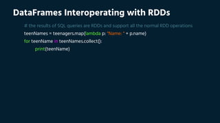
![DataFrame Operations
# # select only the "name" column
df.select("name").show()
# select everybody but increment the age by 1
df.select(df['name'], df['age'] + 1).show()
# select people older than 21
df.filter(df['age'] > 21).show()
# count people by age
df.groupBy("age").count().show()](https://image.slidesharecdn.com/euangeloslinardos20160402apachesparkworkshop-160409103945/85/Apache-Spark-Workshop-Apr-2016-Euangelos-Linardos-67-320.jpg)


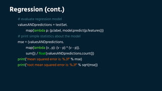
![Regression
from pyspark.mllib.linalg import Vectors
from pyspark.mllib.regression import LabeledPoint
from pyspark.mllib.regression import LinearRegressionWithSGD
def prepareDump(row):
return LabeledPoint(row[0],Vectors.dense((row[1],row[2],...,row[10],row[11])))
# dummy split into train and test set
trainSet = dump.filter(lambda x: x.features[9] <= 4000)
testSet = dump.filter(lambda x: x.features[9] > 4000)
# build regression model: without such a small step size, the algorithm would diverge
model = LinearRegressionWithSGD.train(data=trainSet, iterations=100, step=0.000000001)](https://image.slidesharecdn.com/euangeloslinardos20160402apachesparkworkshop-160409103945/85/Apache-Spark-Workshop-Apr-2016-Euangelos-Linardos-72-320.jpg)
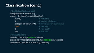
![Classification
# import required libraries
from pyspark.mllib.regression import LabeledPoint
from pyspark.mllib.linalg import Vectors
from pyspark.mllib.tree import DecisionTree
# prepare dump
dump = (dump.
map(lambda line: prepareDump(line)).
map(lambda line: LabeledPoint(line[0],Vectors.dense(line[1]))))](https://image.slidesharecdn.com/euangeloslinardos20160402apachesparkworkshop-160409103945/85/Apache-Spark-Workshop-Apr-2016-Euangelos-Linardos-74-320.jpg)
![Clustering
# import required libraries
from pyspark.mllib.linalg import Vectors
from pyspark.mllib.clustering import KMeans
# convert original data points into dence format
dump = dump.map(lambda line: Vectors.dense(line))
clusters = 2
iterations = 20
model = KMeans.train(dump, clusters, maxIterations=iterations)
# get the centers of the 2 clusters
_2_centers = [tuple(c) for c in model.clusterCenters]](https://image.slidesharecdn.com/euangeloslinardos20160402apachesparkworkshop-160409103945/85/Apache-Spark-Workshop-Apr-2016-Euangelos-Linardos-76-320.jpg)
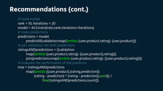
![Recommendations
# import required libraries
from pyspark.mllib.recommendation import Rating, ALS
# dummy split into three sets, namely train, validation and test
train = (ratings.map(lambda x: parseRatings1(x)).
filter(lambda x: (((x[3] % 10) < 6))).
map(lambda x: parseRatings2(x)))
validation = (ratings.map(lambda x: parseRatings1(x)).
filter(lambda x: (((x[3] % 10) >= 6) and ((x[3] % 10) < 8))).
map(lambda x: parseRatings2(x)))
test = (ratings.map(lambda x: parseRatings1(x)).
filter(lambda x: (((x[3] % 10) >= 8))).
map(lambda x: parseRatings2(x)))](https://image.slidesharecdn.com/euangeloslinardos20160402apachesparkworkshop-160409103945/85/Apache-Spark-Workshop-Apr-2016-Euangelos-Linardos-77-320.jpg)


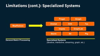
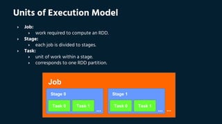
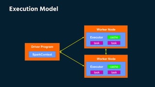
This document outlines a workshop on Apache Spark, detailing the setup environment across different operating systems and providing hands-on training examples. It covers Spark's advantages, architecture, resilient distributed datasets (RDDs), and includes sample codes for operations like word count and data transformation. Additionally, it discusses Spark's performance benefits over MapReduce and the importance of persistence in RDDs for efficient computation.