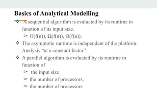
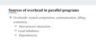
ANALYTICAL MODELS OF
PARALLEL PROGRAMS
Prof. Shashikant V. Athawale
Assistant Professor | Computer Engineering
Department | AISSMS College of Engineering,
Kennedy Road, Pune , MH, India - 411001
Contents
❖ Analytical Models: Sources of overhead in Parallel
Programs.
❖ Performance Metrics for Parallel Systems
❖ The effect of Granularity on Performance
❖ Scalability of Parallel Systems
❖ Minimum execution time and minimum cost
❖ Optimal execution time.
❖ Dense Matrix Algorithms: Matrix-Vector Multiplication
❖ Matrix-Matrix Multiplication.
Basics of Analytical Modelling
❖ A sequential algorithm is evaluated by its runtime in
function of its input size.
➢ O(f(n)), Ω(f(n)), Θ(f(n)).
❖ The asymptotic runtime is independent of the platform.
Analysis “at a constant factor”.
❖ A parallel algorithm is evaluated by its runtime in
function of
➢ the input size
➢ the number of processors,
➢
Sources of overhead in parallel programs
❖ Overheads: wasted computation, communication, idling,
contention.
➢ Inter-process interaction.
➢ Load imbalance.
➢ Dependencies.
Performance metrics for parallel systems
❖ Execution time = time elapsed between
➢ beginning and end of execution on a sequential
computer.
➢ beginning of first processor and end of the last
processor on a parallel computer.
Performance metrics for parallel systems
❖ Total parallel overhead.
➢ Total time collectively spent by all processing
elements = pTp
➢ Time spent doing useful work (serial time) = Ts
➢ Overhead function: To = pTp-Ts.
Effect of Granularity on Performance
❖ Scaling down: To use fewer processing elements than
the maximum possible.
❖ Naïve way to scale down:
➢ Assign the work of n/p processing element to every
processing element.
■ Computation increases by n/p.
■ Communication growth ≤ n/p.
❖ If a parallel system with n processing elements is cost
optimal, then it is still cost optimal with p.
Scalability of Parallel Systems
❖ Scalability: ability to use efficiently increasing
processing power.
❖ Can maintain its efficiency constant when increasing the
number of processors and the size of the problem.
❖ In many cases T0=f(TS,p) and grows sub-linearly with
TS. It can be possible to increase p and TS and keep E
constant.
❖ Scalability measures the ability to increase speedup in
function of p.
Minimum execution time and minimum cost
❖ We can determine the minimum parallel runtime T min P
for a given W by differentiating the expression for TP
w.r.t. p and equating it to zero.
❖ If p0 is the value of p as determined by this equation, Tp
(p0) is the minimum parallel time.
Dense Matrix Algorithms: Matrix-Vector
Multiplication
❖ We aim to multiply a dense n × n matrix A with an n × 1
vector x to yield the n × 1 result vector y.
❖ The serial algorithm requires n2
multiplications and
additions. W = n2
Matrix Vector Multiplication
❖ There are Two Types :
➢ Rowwise 1-D Partitioning
■ The n × n matrix is partitioned among n
processors, with each processor storing complete
row of the matrix.
■ The n × 1 vector x is distributed such that each
process owns one of its elements.
Matrix Vector Multiplication
❖ 2-D partitioning
■ The n × n matrix is partitioned among n2
processors such that each processor owns a single
element.
■ The n × 1 vector x is distributed only in the last
column of n processors.
Matrix-Matrix Multiplication
❖ The problem of multiplying two n × n dense, square
matrices A and B to yield the product matrix C = A × B.
❖ The serial complexity is O(n3
).

Analytical Models of Parallel Programs

  • 1.
    ANALYTICAL MODELS OF PARALLELPROGRAMS Prof. Shashikant V. Athawale Assistant Professor | Computer Engineering Department | AISSMS College of Engineering, Kennedy Road, Pune , MH, India - 411001
  • 2.
    Contents ❖ Analytical Models:Sources of overhead in Parallel Programs. ❖ Performance Metrics for Parallel Systems ❖ The effect of Granularity on Performance ❖ Scalability of Parallel Systems ❖ Minimum execution time and minimum cost ❖ Optimal execution time. ❖ Dense Matrix Algorithms: Matrix-Vector Multiplication ❖ Matrix-Matrix Multiplication.
  • 3.
    Basics of AnalyticalModelling ❖ A sequential algorithm is evaluated by its runtime in function of its input size. ➢ O(f(n)), Ω(f(n)), Θ(f(n)). ❖ The asymptotic runtime is independent of the platform. Analysis “at a constant factor”. ❖ A parallel algorithm is evaluated by its runtime in function of ➢ the input size ➢ the number of processors, ➢
  • 4.
    Sources of overheadin parallel programs ❖ Overheads: wasted computation, communication, idling, contention. ➢ Inter-process interaction. ➢ Load imbalance. ➢ Dependencies.
  • 5.
    Performance metrics forparallel systems ❖ Execution time = time elapsed between ➢ beginning and end of execution on a sequential computer. ➢ beginning of first processor and end of the last processor on a parallel computer.
  • 6.
    Performance metrics forparallel systems ❖ Total parallel overhead. ➢ Total time collectively spent by all processing elements = pTp ➢ Time spent doing useful work (serial time) = Ts ➢ Overhead function: To = pTp-Ts.
  • 7.
    Effect of Granularityon Performance ❖ Scaling down: To use fewer processing elements than the maximum possible. ❖ Naïve way to scale down: ➢ Assign the work of n/p processing element to every processing element. ■ Computation increases by n/p. ■ Communication growth ≤ n/p. ❖ If a parallel system with n processing elements is cost optimal, then it is still cost optimal with p.
  • 8.
    Scalability of ParallelSystems ❖ Scalability: ability to use efficiently increasing processing power. ❖ Can maintain its efficiency constant when increasing the number of processors and the size of the problem. ❖ In many cases T0=f(TS,p) and grows sub-linearly with TS. It can be possible to increase p and TS and keep E constant. ❖ Scalability measures the ability to increase speedup in function of p.
  • 9.
    Minimum execution timeand minimum cost ❖ We can determine the minimum parallel runtime T min P for a given W by differentiating the expression for TP w.r.t. p and equating it to zero. ❖ If p0 is the value of p as determined by this equation, Tp (p0) is the minimum parallel time.
  • 10.
    Dense Matrix Algorithms:Matrix-Vector Multiplication ❖ We aim to multiply a dense n × n matrix A with an n × 1 vector x to yield the n × 1 result vector y. ❖ The serial algorithm requires n2 multiplications and additions. W = n2
  • 11.
    Matrix Vector Multiplication ❖There are Two Types : ➢ Rowwise 1-D Partitioning ■ The n × n matrix is partitioned among n processors, with each processor storing complete row of the matrix. ■ The n × 1 vector x is distributed such that each process owns one of its elements.
  • 12.
    Matrix Vector Multiplication ❖2-D partitioning ■ The n × n matrix is partitioned among n2 processors such that each processor owns a single element. ■ The n × 1 vector x is distributed only in the last column of n processors.
  • 13.
    Matrix-Matrix Multiplication ❖ Theproblem of multiplying two n × n dense, square matrices A and B to yield the product matrix C = A × B. ❖ The serial complexity is O(n3 ).