An iterative method for solving nonlinear Riemann Hilbert problems.pdf

Journal of Computational and Applied Mathematics 29 (1990) 311-327
North-Holland
311
An iterative method for solving nonlinear
Xemann-Hilbert problems
Elias WEGERT
Sektion Mathematik, Bergakademie Freiberg, Akademiestrah’e 6, 9200 Freiberg, GDR
Received 20 October 1988
Revised 6 March 1989
Abstract: A geometrically motivated linearization is used to construct an iterative method for solving nonlinear
boundary value problems for holomorphic functions. The nondiscrete method is quadratically convergent. Results of
some test calculations are reported.
Keywords: Newton method, Riemann-Hilbert problem, conformal mapping, singular integral equations.
0. Introduction zyxwvutsrqponmlkjihgfedcbaZYXWVUTSRQPONMLKJIHGFEDCBA
In the last few years several authors proposed iterative methods for computing conformal
maps which make use of the easy construction of the solutions to linear Riemann-Hilbert
problems ([5,7,11-131; cf. also [4, g16.91 and the systematizing paper [2] by Gutknecht which
contains many further references).
The objective of the present paper is to extend Wegmann’s method for numerical conformal
mapping to a much wider class of strongly nonlinear Riemann-Hilbert problems. These
problems arise in different branches of mathematics as well as in applications. The close
connection of Riemann-Hilbert problems with certain classes of singular integral equations
(which involve, for instance, the Theodorsen integral equation, see [14]) is known classically.
Recently, in [9], we found relations to certain extremal problems which occur, for example, in
H”-optimization problems [3]. The paper [lo] treats an application in hydromechanics.
The iteration method considered here is based on a geometrically motivated linearization of
the boundary condition. In each step a linear Riemann-Hilbert problem must be solved, whose
solution, however, is available in a closed form. The nondiscretized method is locally quadrati-
cally convergent.
If fast Fourier transform is used to evaluate a discrete approximation to the solution of the
linear Riemann-Hilbert problems on a uniform mesh the costs are of order O(N log N) per
iteration.
Discretization brings up new effects for which some heuristic explanations are given. A more
detailed investigation is postponed to a forthcoming paper.
0377-0427/90/$3.50 0 1990, Elsevier Science Publishers B.V. (North-Holland)

312 E. Wegert / Riemann-Hilbert problems zyxwvutsrqponmlkjihgfedcbaZYXWVUTS
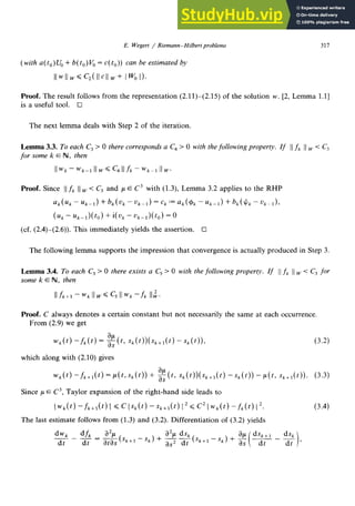
For the convenience of the reader we summarize results about the solvability of Riemann-Hil-
bert problems in the first section. In Sections 2 and 3 the algorithm is described and the
convergence of the iteration is proved. Section 4 deals with aspects of the numerical implementa-
tion. Finally, in Section 5, the results of some test calculations are reported. zyxwvutsrqponmlkjihgfedcbaZY
1. Riemann-Hilts probtems
Let H” zyxwvutsrqponmlkjihgfedcbaZYXWVUTSRQPONMLKJIHGFEDCBA
n C be the space of functions holomorphic in the unit disk lD and continuous up to
its boundary T. We use the terminology Riemann-Hilbert problem (RHP) to denote the
following boundary value problem:
Given a function F: U x R X W + IF& find all functions w = u + iu E H” n C satisfying the
boundary condition
F(t, u(t), u(t)) =o V’tE lr. (1.1)
Of particular interest is the linear RHP with the boundary condition
~(~)~(~~ + ~(~)U~~~ = c(t) vt E lr.
After introducing the curves
M,:={u+iuEQ::F(t, u, o)=O}, tEU,
the relation (1.1) can be written as
W@)EM, VfElr,
which stresses the geometric nature of this problem.
Sometimes it is more convenient to replace (1.2) by a parametric representation
Ml:= {u+iuEd=:u+iu=p((t, s), sflw}.
O-2)
It is supposed that p : + X K! + C belongs to the smoothness class C’ and satisfies an estimate
(1.3)
with a positive constant C.
We speak of a RHP of type A if all curves M, are homeomo~~c to the unit circle. In this
case it is assumed that ,u is periodic in s. The RHP is said to be of type B if all curves M, are
homeomorpbic to the real line.
We summarize some results about the solvability of RHPs and first treat problems of type A.
The above assumptions alone do not guarantee the existence of solutions. We here confine
ourselves to a simple case and require, in addition, that the origin lies in the interior of all curves
M*:
OEint M, VdtEU.
What this condition is needed for is discussed in detail in [8,9]. We remark that the iteration
method is also applicable to RHPs with regularly holomorphically traceable { M,}, see 191.
The next theorem is (in a somewhat different setting and under slightly stronger assumptions)
due to Snirel’man [6]; cf. also [8] for an alternative proof.

E. Wegert / Riemann-Hilbert problems 313 zyxwvutsr
Theorem 1.1. Under the assumptions of Problem A, for any choice oft, E U, W, E M,,, z,, . . . , z, E
IlIDthere exists exactly one function w E H” n C satisfying the following conditions:
w(t) E X vt E T ( boundary condition ),
43) = w, (initial condition),
w(z/J = 0, zyxwvutsrqponmlkjihgfedcbaZYXWVUTSRQPONMLKJIHGFEDCBA
k= l,...,n, ( interpolation conditions ),
wind w=n.
Here and in the following wind w denotes the winding number of the boundary function of w
about the origin. By the argument principle, the last two conditions ensure that w has exactly the
zeros zi, . . . , z, in [ID.
As is shown in [6,8], a simple transformation sends the solutions with wind w > 0 to solutions
with wind w = 0 of a related problem. Therefore only solutions without zeros in IID are
considered henceforth.
When dealing with RHPs of type B, we assume in addition some regularity assumptions at
infinity, namely, we suppose that the limits
v’(t) := lim
s+*,%~
4,
1 al-J
lim zyxwvutsrqponmlkjihgfedcbaZYXWVUTSRQPONMLKJIHGF
--(t, s) =0
s_+m s2 at
exist uniformly in t.
The solvability of RHPs of type B depends significantly on the index
K := wind v+ = wind v-.
A little refining of the techniques employed in the proof of [8, Theorem 31 yields the following
result. 1
Theorem 1.2. Let the assumptions of Problem B be fulfilled.
(i) If zyxwvutsrqponmlkjihgfedcbaZYXWVUTSRQPONMLKJIHGFEDCBA
K c 0, then there exists at most one function w E H” n C satisfying
w(t)EM* V,‘tElr. (1.4)
(ii) If K = 0, then f or any choice of t, E T and W, E MI, there exists exactly one function
w E H” n C satisfying (1.4) and
w(t,) = w,. (1.5)
(iii) If K > 0, then for any choice oft, E T, W, E M,(], zl,. . . , z, E D and W,, . . . , W, E Q=there
is exactly one solution w E H” n C of (1.4), (1.5) which satisfies
w(q) = W,, k=l,...,K. 0 4
The case K > 0 can easily be reduced to the case K = 0 and therefore we shall take K = 0 in the
sequel.
Remark 1.3. In either case the solutions belong to H” n Wd, 1 <p < 00, the space of holomor-
phic functions with boundary functions in the Sobolev space W,‘(T). Henceforth we shall work
in Ha n W:.
’ We take the opportunity to remark that the second condition in (*) is missing (but needed) in [8].

314 zyxwvutsrqponmlkjihgfedcbaZYXWVUTSRQPONMLKJIHGFEDCBA
E. W egert / Riemann-Hiibert problems
Remark 1.4. zyxwvutsrqponmlkjihgfedcbaZYXWVUTSRQPONMLKJIHGFEDCBA
The points zi,. . . , z, are assumed to be pairwise distinct, but the results can be
modified in the usual way if points coincide.
Remark 1.5. Conformal mapping can be used to extend the results to arbitrary smoothly
bounded simply-connected regions G in place of D. To calculate the solutions of RHPs on a
domain G, the needed conformal map of D onto G can be determined in a preceding step with
the same iteration method since conformal mapping is a special RHP of type A.
Remark 1.6. Frequently one has to solve the RHP with the boundary condition w(t) E h4, and
one of the side conditions
Re w(0) = I!& (I -7)
or
Im w(0) = V, (1.8)
at the origin (instead of an initial condition). The existence of solutions to these problems is
discussed in [8,9,15], for instance. Here we assume the existence of a solution w = w0 correspond-
ing to U, := U,, or V, := V,, respectively. By replacing the curves it4, by straight lines tangent to
44, at w,,(t) we arrive at a linear RHP a,,( t)u( t) + b,(t) U(t) = c,,(t) and put
6, := & J
2”arg( b, - iao)(eiT) d7. zyxwvutsrqponmlkjihgfedcbaZYXWVUTSRQPONMLKJIHGFE
0
(1.9)
If S, # 37 (mod a) the problem w(t) E M, with the side condition (1.7) has a solution w if
1U, - U, 1 is sufficiently small. This solution is the only solution in a certain neighborhood of
w 0. The RHP with the side condition (1.8) is locally uniquely solvable (in this sense) if So # 0
(mod T) and 1V, - V,, 1 is sufficiently small.
2. The algorithm
The iterative method applies without any changes to both types of RHPs if we look for
solutions w0 of
w(t) EM, VfEU, (2.1)
w(4)) = w, E Mt,, (2.2)
and assume wind w. = 0 for problems of type A and K = 0 for problems of type B, respectively.
This hypothesis ensures that the winding number of the function a + ib is zero, where
(a + ib)( t) is the unit vector normal to 44, at wo( t).
To avoid complications we let the parametric representation p satisfy wind ap/ a.s( *, 0) = 0
for problems of type A. Then wind a~/ &( e, s( e)) = 0 for any continuous function s : T + R, as
can easily be shown using standard arguments from topology.
Next we are going to construct two sequences { zyxwvutsrqponmlkjihgfedcbaZYXWVUTSRQPONMLK
fk} and { wk} of functions, which belong to
the Sobolev space W:(T) if p E C2(T X Iw), which is assumed henceforth. The functions fk
satisfy the relation fk(t) E M,, t E T, and f( to) = W,. In general these functions are not
holomorphically continuable into [ID.The functions wk are solutions of the linear RHPs which
emerge from replacing the curves M, by tangents to M, at fk(t). These functions can be
extended holomorphically into 119,
but they do not fulfil relation (2.1). In the next section it will
be shown that both sequences { fk} and { wk} converge to the solution of (2.1), (2.2).

E. Wegert / Riemann-Hilbert problems 315
Step 1 zyxwvutsrqponmlkjihgfedcbaZYXWVUTSRQPONMLKJIHGFEDCBA
(initial function). Choose a real-valued function s, zyxwvutsrqponmlkjihgfedcbaZYXWVUTSRQPO
n W:(U) with p( t,, sl( to)) = W, and
calculate fi = +i + i#i : lJ + C from
f*(t) := / J
FL(t>
s&)). (2.3)
Put k := 1.
Step 2 (linear RHP). Determine akr b,, ck : T -+ R! from
a,(t) := Img(t, Sk(t)),
bk(t):= -Re!$(t, Sk(t)),
c/t(t):=adth(t) +b,(tbk,(t).
Solve the linear RHP for the function wk = uk + iv,:
a,(+&) + b&)0&) = c,&),
WkGO) = 6.
Step 3 (projection). Let sk+i : T + R be given by
G+*(t) := GO) + (W/ A) -f,O))&(t~ %(G)
and determine fk+i = $~~+i+ i#k+l : U + C from
A+&) := CL@, Sk+&))*
Put k := k + 1 and repeat beginning with Step 2.
(2.4)
(2.5)
(2.6)
(2.7)
(2.8)
(2.9)
(2.10)
Remark 2.1. If the index wind( ak + ib,) of the linear RHP (2.7) is zero and if the coefficients are
normalized by 1ak + ib, 1= 1, the solution wk of (2.7), (2.8) is given by the following set of
formulas (we omit the subscripts):
U(t) := arg(b(t) - ia(t u(t) := H C(t), (2.11)
i?(t) := -a(t) exp ii(t), ii(t) := b(t) exp E(t), (2.12)
C(t):=c(t) exp(-C(t)), C(t) :=Hv^(t), (2.13)
d:= (U,b(t,) - Ga(t,)) exp(-G(t,)) - G(t,), (2.14)
w := (ii + ifi)(i; + iu^
+ d), (2.15)
with U, + iv, = W,. H denotes the singular integral operator with Hilbert kernel which assignes
to a function v (the negative of) its conjugate function Hv:
H zyxwvutsrqponmlkjihgfedcbaZYXWVUTSRQPONMLKJIHGFEDCBA
v(e”) = &k2‘v(ei”) cot +(o - 7) do.
The integral has to be interpreted in the Cauchy principal value sense.
Remark 2.2. Using that H is bounded in W:(T) and taking into account the mapping properties
of the superposition operator with differentiable functions (cf., for instance, [2, Lemma 1.11) it is

316 E. Wegert / Riemann-Hilbert problems zyxwvutsrqponmlkjihgfedcbaZYXWVUTSR
not hard to see that a, b, c E W:(T) implies w E W&T). It follows by induction that all
functions sk belong to W:(T) and, according to the remark at the beginning of this section,
wind( ak + ib,) = 0 for all k. Hence the iteration can be performed. zyxwvutsrqponmlkjihgfedcbaZYXWVUT
Remark 2.3. The linear RHP (2.7) with wind( ak + ib,) = 0 and either of the side conditions (1.7),
(1.8) is uniquely solvable if 6 # &T (mod IT) in the case of condition (1.7) and 6 f 0 (mod T) for
condition (1.8); here S is defined according to (1.9). The solution is given by (2.11)-(2.13) and
(2.15) with
d := U, + 77sin 6
cos 6
(2.16)
for condition (1.7) and
d.= P-o-)7 cos 6
sin 6
(2.17)
for condition (1.8). Herein
1
JzyxwvutsrqponmlkjihgfedcbaZYXWVUTSRQPONMLKJIHGFEDCBA
277
77”G o iT(eiT) dr.
Remark 2.4. There is another way to determine solutions of RHPs with wind w = n > 0 (Problem
A) or of RHPs with K > 0 (Problem B) without transforming the problem. This can be done by
linearizing the boundary condition as above and by solving the linear RHPs with the initial
condition and the interpolation conditions of the original problem. In case of Problem A one has
to start the iteration with a function fi satisfying wind fi = n. The iteration can be performed if
fi is sufficiently close to the exact solution.
3. Convergence
The norms in L,(T), C(U),W:(U) are denoted by 11
* 11
L, 11
. II c, II - II w.
Theorem 3.1. Let loE C3(U x R). Then there exist positive numbers e and C with the following
properties. If IIfi - w. IIw < e, then both sequences { fk } and { wk } converge in W:(U) to the
solution wo. The error can be estimated by zyxwvutsrqponmlkjihgfedcbaZYXWVUTSRQPONMLKJIHGFED
IIfk+l -wo IIw~c IIfk-wo II& (3 -1)
The proof of Theorem 3.1 is prepared by five lemmas. The first one concerns an a priori
estimate for the solutions of the linear RHP.
Lemma 3.2. For each C, > 0 there exists a constant C, > 0 with the following properties. If
& < a2(t) + b2(t) < C,, IIa IIWGc ,, IIb IIWGc ,, wind( a + ib) = 0,
1
then the solution w E H” n W: of the Riemann-Hilbert problem
a(t)u(t) + b(t)v(t) =c(t),
u(t,) + iv(to) = W, (=: U, + iv,)

(with a(to)Uo + b(t,)V, = c(t,)) can be estimated by zyxwvutsrqponmlkjihgfedcbaZYXWVUTSRQPONMLK
II~IIw~c *(IIc IIw+ VW>. zyxwvutsrqponmlkjihgfedcbaZYXWVUTSRQPONMLKJIHGFEDCBA
Proof. The result follows from the representation (2.11)-(2.15) of the solution W. [2, Lemma 1.11
is a useful tool. 0
The next lemma deals with Step 2 of the iteration.
Lemma 3.3. To each C, > 0 there corresponds a C, > 0 with the following If 11
fk 11
W < C,
for some k E N, then
11
wk zyxwvutsrqponmlkjihgfedcbaZYXWVUTSRQPONMLKJIHGFEDCBA
wk-l II Pi’< c4 11 fk - wk-l IIWe
Proof. Since 11
fk IIw < C, and p E C3 with (1.3), Lemma 3.2 applies to the RHP zyxwvutsrqponmlkjihg
ak(Uk - uk-l) + bkbk - uk-l ) = ck:= ak(+k - uk-l) + bk(+k - uk4>,
(Uk-Uk-l)(tO)+i(Uk-Uk-l)(tO)=o
(cf. (2.4)-(2.6)). This immediately yields the assertion. q
The following lemma supports the impression that convergence is actually produced in Step 3.
Lemma 3.4. To each C, > 0 there exists a C, > 0 with the following property. If IIfk 11
w < C, for
some k E N, then
IIfktl - wk IIW G c5 IIwk -fk 11;.
Proof. C always denotes a certain constant but not necessarily the same at each occurrence.
From (2.9) we get
%
Wk(t) -fkb) = a,(‘> Sk(t))(Sk+l(t) - sk<t>>, (3.2)
which along with (2.10) gives
Wk(t) -fk+#) = @, zyxwvutsrqponmlkjihgfedcbaZYXWVUTSRQPONMLKJIHGFEDCBA
Sk(t)) + $$ Sk(t))(Sk+l(t) -Sk(t)) - dt, Sk+l(t)). (3*3)
Since p E C3, Taylor expansion of the right-hand side leads to
i W&) -.fk+,(t) 1 G c lSk(d - Sk+l(t) 1 2 d c2 1 Wk(t) -fk@) 12-
The last estimate follows from (1.3) and (3.2). Differentiation of (3.2) yields
(3.4)
dw, dfk a2P
-(s Sk)+ ~~(sk+~-sk)+
2/J
---=
dt dt zyxwvutsrqponmlkjihgfedcbaZYXWVUTSRQPONMLKJIHGFEDCBA
at as k+l- as2 dt

318 E. Wegert / Riemann-Hilbert problems zyxwvutsrqponmlkjihgfedcbaZYXWVUTS
whence
II
ds kfl
dt
- 2 iIwk-fk ii&V+ iIsk+l-skIIL+
On the other hand, by differentiating equation (2.10) we obtain
-skiIC .
i
(3.5)
+) = $(& s,(t)) + $, s,(t))~(t),
which implies
< c(1 + 1)fk 11
W) < c2.
L
Using (1.3) and (2.9) we arrive at the inequalities zyxwvutsrqponmlkjihgfedcbaZYXWVUTSRQPONMLKJI
IIsk+l - sk 11C G c iI wk -fk II C G c2 11wk -fk II W,
and (3.5)-(3.7) together produce the estimate
ds kil
dt
- 2 zyxwvutsrqponmlkjihgfedcbaZYXWVUTSRQPONMLKJIHGFEDCBA
I/
~ciIwk-fk IIN’.
L
(3.6)
(3.7)
(3.8)
From (3.3) we conclude, by differentiation,
d’+‘, dfk+l
---
dt dt
= $(., Sk) + g(., sk)% + $., sk)(sk+l -‘k)
d2P
+ j--$.9 sk)$(sk+I
al-l
-Sk) + ,,(., Sk)
al-l
--
at
(-9 Sk+l) - $*Y sk+,)w
=11+12+13,
where
P-9)
I,:= $(‘, Sk) - $(., sk+i) + g(. ’ sk)(sk+l - sk)y
ap ap a%
,,(*, Sk) - z(.> sk+l) + j-$*? sk)(sk+, -sk) $3
I
ap ap
j-$, Sk) - j$ zyxwvutsrqponmlkjihgfedcbaZYXWVUTSRQPONMLKJIHGFEDCBA
sk+l
)I[
ds,,,
dsk
-
-~
1
dt dt .
In view of (3.7), (3.6) and (3.8), Taylor expansion of Ii, I,, IX yields
11
I, 11
L G c 11Sk+1 - sk 112:G c2 11wk -fk Ihi’,
bk+l-skll:~c21iwk-fkiI&
L
II
dSk+l
(I~,I~L~cI~sk+,-skIIC 7 - 2
I/
<c2jIwk-fk iI;*
L

Taking into account (3.9) we obtain
Combining the latter estimate and (3.4) completes the proof. •I zyxwvutsrqponmlkjihgfedcbaZYXWVUTSR
Lemma 3.5. For each C, > 0 there exists a C, > 0 with the following properties:
(9 IIfkIIW<C3 * IIfk+l-~kIIW~~6IIfk-~~-~II~~
(ii) IIfk zyxwvutsrqponmlkjihgfedcbaZYXWVUTSRQPONMLKJIHGFEDCBA
IIWCc 3, IIfk+l II WC c3 =$ IIwk+l -f/S+, II w G G II w/c-fk II&
Proof. (1) Using Lemma 3.4 and Lemma 3.3 one gets the estimates
IIfk+l - wk 11WG c5 II wk -fk hi’
~c5(IIwk- zyxwvutsrqponmlkjihgfedcbaZYXWVUTSRQPONMLKJIHGFEDCB
wk-l Ii W+ 11 wk-l -fk II WI*
G c5(1 + c4)2 II fk - wk-l Ihi’.
(2) Applying Lemma 3.3 and Lemma 3.4 once more, we conclude
II wk-t1 -fk+l II W G II wk+l - wk II W + II wk zyxwvutsrqponmlkjihgfedcbaZYXWVUTSRQPONMLK
-fk+l iI W
G t1 + c4> II wk -fk+l IIW
6 c5(1 + c4) 11wk -fk Ihi’* q
Lemma 3.6. Put C, = IIw. IIw + 1 and let C,, C, be determined in accordance with Lemma 3.3 and
Lemma 3.5. Let further c be given by
f = 2 max{ C,, C,(l + C,), 2(1 + C4)}. (3.10)
Then, starting the iteration with any function fl such that
Ilfl -woII WCC,
the sequences { fk }, { wk } satisfy the estimates
IIfkIIW< IIw,Il~+l-3.2-~-‘<C3, k> 1,
IIfk+l - wkIIW~311fk-Wk-lII~<2-k-2, k>l,
IIwk -fk II WG t/I wk-l -fk-1 II W<2-k-‘, k>, 2.
Proof. (1) By definition of c,
(3.11)
(3.12)
(3.13)
(2)
(3)
IIfi II w G II wo II w + IIfl - wo II w < II wo II w + 6 G II wo II w + + < c,. (3.14)
From Lemma 3.3 we derive that
IIWl -fi IIWG IIf1-woIIw+ IIW1-WoIIw~(1+C~)Ilfl-woIIw<~(1+C~)~~~
(3.15)
Because of (3.14), Lemma 3.5(i) applies to k = 1. Hence
IIf* - w1 II w G c, IIfi - wo llczG c,c IIfl - wo II w G i IIfi - wo IIw < i. (3.16)

320 E. Wegert / Riemann-Hilbert problems
(4) From (3.14)-(3.16) the following estimates result:
II zyxwvutsrqponmlkjihgfedcbaZYXWVUTSRQPONMLKJIHGFEDCBA
f2 IIw G IIf2 - Wl IIw+ zyxwvutsrqponmlkjihgfedcbaZYXWVUTSRQPONMLKJIHGFEDCBA
IIWl-f1 II w+ IIfl IIw < + + i + i + IIwoIIw
= 11
w. 11
w+ 1 - i < c ,. (3.17)
(5) The estimates (3.14), (3.17) guarantee that Lemma 3S(ii) with k = 1 is applicable. This in
conjunction with (3.10), (3.15) gives that
IIzyxwvutsrqponmlkjihgfedcbaZYXWVUTSRQPONMLKJIHGFEDCBA
w2 zyxwvutsrqponmlkjihgfedcbaZYXWVUTSRQPONMLKJIHGFEDCBA
-f2 IIWG G IIWI-f1 Ilk GO + C&II Wl-f1 IIw< ill Wl -f1 II WC i.
(6) As we have just shown, (3.11), (3.12) hold for k = 1 and (3.13) is true for k = 2. Now
Lemma 3.6 can be proved inductively by repeating the steps (3), (4) and (5). Cl zyxwvutsrqponmlkjihgfed
Proof of Theorem 3.1. (1) From Lemma 3.6 we conclude that if k < m,
Ilfk-fm IIWG Ilfk-wkIIw+ IIwk-fk+l Ilw+ ..* +IIWm-l-fm llw~3°2-k-‘.
Therefore {fk } converges in W:(U) to a certain function fo. Because of (3.13) the sequence
{ wk } also converges to f. in IVY. Since all functions fk satisfy the boundary condition (2.1)
and the initial condition (2.2), this is also true for fo. On the other hand, the functions wk can be
extended holomorphically into [IDand thus f. has the same property. So f. coincides with wo,
the only solution of the RHP (2.1), (2.2).
(2) To prove the error estimate of Theorem 3.1 we use Lemma 3.4 and Lemma 3.6:
IIfk+l -fk IIWG iI fk+l - wk II W+ II wk -fk II WG c II wk -fk II W
G c2 11wk-l -fk-1 II& (3.18)
If k is sufficiently large, Lemma 3.4 yields
11
fk -fk-1 IIWa 11 zyxwvutsrqponmlkjihgfedcbaZYXWVUTSRQPONMLKJIHGFEDCBA
wk-l -fk-1 iI W - 11fk - wk-l 11W
2 II wk-l -fk-1 II W- cII wk-l -fk-1 Ihi
> (1 - c 11
wk-1 -fk-1 IIW > iI wk-l -fk--l 11Wa :I1 wk-l -fk-1 IIW .
(3.19)
Combine (3.18) and (3.19) to obtain
11
fk+l -fk 11
W G c 11fk -fk-1 hi’.
Now let x := 11
fk - fktl IIw G 1/(3C). From (3.20) the estimate
11
fk+l - wO II WG II fk+l -fk+2 II W+ II fk+2 -fk+3 iI W+ . . ’
< cx2 + c3x4 + c7xs + . . *
< cx2(1+ 3-l + 3-2 + - *. ) = :cx2
follows. On the other hand,
(3.20)
(3.21)
11
fk - wO II Wa Ii fk -fk+l IW - II fk+l - wO II W a x - +cx2 a ix.
The relations (3.21) and (3.22) prove (3.1) (with a new constant C). 0
(3.22)
Remark 3.7. In fact the assumption p E C 2 is sufficient for the convergence of the iteration
method in We. A proof of this, however, requires more careful estimations. The convergence

E. Wegert / Riemann-Hilbert problems 321 zyxwvut
is at least superlinear, i.e., for each 4 with 0 < q -c 1 there exists a positive number C such that
IIfk - woIIWG Qk. zyxwvutsrqponmlkjihgfedcbaZYXWVUTSRQPONMLKJIHGFEDCBA
Remark 3.8. Theorem 3.1 remains in force for a modified iteration method for solving RHPs with
the side conditions (1.7) or (1.8) if 6, # HIT(mod IT) or 8, # 0 (mod T), respectively. For solving
the corresponding linear RHPs of Step 2 one only has to replace the constant d from the
formula (2.14) by d from (2.16) or (2.17), respectively (cf. Remarks 1.6 and 2.3). The solvability
of the linear RHPs is ensured if zyxwvutsrqponmlkjihgfedcbaZYXWVUTSRQPONMLKJIHGFEDCBA
fi is sufficiently near to wO.
The same can be said of the modified methods from Remark 2.4.
4. Implementation
The iteration can be performed numerically by replacing all functions needed in the iteration
process by their values on a grid of equidistant points
k=O, l,..., N-l.
If, conversely, the values of a function f at the discretization points are known, the whole
function can be reconstructed approximately by trigonometric interpolation.
The discretization of Step 3 causes no difficulties. Its computational expense is of order O(N)
for one iteration step.
The crucial point is the discretization of Step 2. For approximately solving the linear RHP one
has several possibilities.
In his paper [13], Wegmann proposed two methods for solving the discrete linear RHP. The
first one is based on a conjugate gradient method in combination with fast Fourier transform
(FFT) and has cost of order O( N log N). The second method leads to a system with a Toeplitz
matrix, for which fast solvers with cost 0( N log*N) are available. It needs FFT again.
We have performed calculations with a more naive third method (also used by Wegmann in
[11,12] for conformal mapping). It works directly with the representation (2.11)-(2.15) of the
solution where all functions are calculated only at the points t, and the operator H is replaced
by an operator HN which acts on the values of the functions on the grid. This method is simpler
to implement on a computer, but it should be mentioned that it yields only approximately a
method of Newton type. On the contrary, Wegmann’s discretization in [13] gives a discrete
Newton method and we suspect that it shows better convergence (cf. the remarks in [13]
concerning conformal mapping and the discussion at the end of our paper).
For calculating the operator HN we used Wittich’s method (cf. [l]). To outline this method we
assume that N is even. Then there exists exactly one trigonometric polynomial
fN fN- 1
c ak cos k7 + c b, sin k7, zyxwvutsrqponmlkjihgfedcbaZYXWVUTSRQPONMLKJIHGFEDCB
k =O k=l
which takes given values uk at t,, k = 0, 1,. . . , N - 1. The coefficients ak and b, can be

calculated by discrete Fourier transform. After rearranging the coefficients in accordance with
the relations
H[l] =o, H[sin /CT] =cos k7, H[cos k7] = -sin kr, k= 1, 2,...,
a second Fourier transform gives the values of the (discrete) conjugate function. In this way we
define
where I means interpolation and R restriction to the discretization points. If N is a power of 2,
the computation can be carried out by FFT with cost of order 0( N log N) (see [4, p.61).
The realization of Step 1 also involves some problems, since a function fi is needed which is
not too far from the unknown solution wO. The best expedient in this situation is to couple the
iteration method with an imbedding method. So one has to construct a family of RHPs
w(t) E Mp, 0 < p < 1, with h4,’ = M,, whose solution for p = 0 is known. Under certain not very
restrictive assumptions (cf. [9]) the solution to the RHPs depends continuously on the parameter
p, Suitable construction of Mp ensures that the e from Theorem 3.1 is bounded, away from zero
(it can be calculated explicitly in terms of M,). Hence one may choose a sequence pO =
0, Pl,. . -7 pm-I, p, = 1 of parameters such that the last approximative solution of the foregoing
problem gives an initial solution for the following one which is sufficiently good to guarantee
convergence of the iteration.
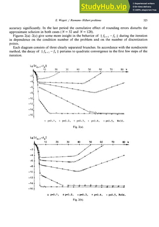
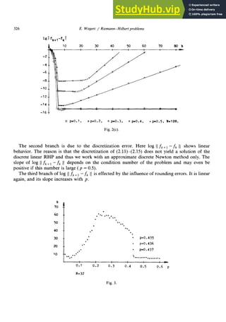
In accordance with the behavior of the nondiscrete iteration method, the values of I] zyxwvutsrqponmlk
fk+1- fk 11
of the discrete version decrease very rapidly as long as the discretization error can be neglected.
After a (possible) period of nearly linearly decreasing values those values begin to increase,
which offers a simple criterion for stopping the iteration. Unfortunately this criterion seems not
to be good, at the very least under the aspect of time saving. We shall have to say a bit more
about this in the last section.
Practical experience has shown that rapidly oscillating errors prevent the convergence of the
iteration, especially for badly conditioned problems. This can lead to increasing I]fk+l - fk 11
although the precision which could be expected is still not obtained. Therefore we recommend to
provide for a possibility of damping these oscillations, for instance by truncation of the highest
Fourier coefficients. This will be illustrated in the final section. zyxwvutsrqponmlkjihgfedcbaZYXWVUTSRQ
5. Examples
We have tested the iteration method for several examples of both types. Two of them will be
employed to present some of our experiences.
The first example is a problem of type A which arises from conformal mapping of the unit
disk onto a family of reflected ellipses {Gp }. The boundaries aG, are given by
aG, := (w = p,(s) eiS, s E [0, HIT)),
with
p,(s):=(1+(p~-2p)cos~s)1’2, O<p<l.

If we look for conformal maps which take z = 0 to w = 0 and z = 1 to w = 1 -p, the exact
mapping function is determined by the correspondence
tan s = (1 -p) tan 7, t = eiT,
of the boundary parameters.
Since simple conformal maps are related to the solutions of the RHP w(t) zyxwvutsrqponmlkjihgfedcbaZ
E dG with winding
number one, we seek the function w0 defined by w,,(z) := z- ’fi,,( z) instead of the conformal
mapping function GO. The resulting new RHP for the function w0 has the boundary condition
w,(t) E M; := t-‘GIG,,,
and the initial condition
w,(l) = 1 -p.
A well-fitted parametric representation for IV/’ is
p,(t, s) = p,(s + 7) exp(is), t = exp(ir), s E Iw.
If p = 0, then all curves Mp are unit circles and w0 = 1 is the solution of the RHP. The
condition number of the problem increases with p. We gave p successively the values p = 0.2,
0.4, 0.6, 0.8 and used the solution of the foregoing problem to construct the initial function for
the following one.
The iteration was cancelled as soon as 11 zyxwvutsrqponmlkjihgfedcbaZYXWVUTSRQPONMLKJIHG
fk+1- fk 11
c (computed as the maximum over the
discretization points) did not decrease.
The results are summarized in Table 1. The first column contains the number of iterations
needed till zyxwvutsrqponmlkjihgfedcbaZYXWVUTSRQPONMLKJIHGFEDCBA
IIfk+l -fk IIc increases. In the second column the minimal values of this norm are
listed and the error at the end of the iteration is given in the third column.
The last three lines with an asterisk reflect the results obtained with damping of rapid
oscillations. Here we listed the number of iterations which are performed after cutting off one
half of the Fourier coefficients.
The second example concerns a RHP of type B. A parametrization of the curves M/’
(involving p as an additional parameter) is
p,(t, s)=s+i(2ps*+cos 7-2~ sin*T), t=exp(ir). zyxwvutsrqponmlkjihgfedcbaZYXWVUTSR
Table 1
log, N p = 0.2 p = 0.4 p = 0.6 p = 0.8
k INCR ERR k INCR ERR k INCR ERR k INCR ERR
4 13 3.4.10p6 5.1.10p5 17 4.9.10-14 1.8.10p3 12 l.O.lO-‘” 2.2.10p2 2 5.8.10-2 1.4.10-l
5 11 4.9.10-16 7.8.10-9 15 1.6.10-14 6.9.10-6 11 4.3.10-” 8.8.10-4 2 2.9.10-l 2.3.10-l
6 5 1.5~10-‘5 1.1~10-‘5 12 4.5.10-‘5 l.l.lo-‘” 9 9.3.10-‘2 1.1.10-6 2 2.1.10-l 1.3.10-l
7 7 6.6.10_16 1.7.10-‘5 5 2.2.1Or” 5.1.10r15 6 1.4.10-12 1.7.10p’2 3 2.3.10-2 2.4.10p2
8 5 1.1.10-15 2.2.10-15 7 1.4.10-15 8.4.10p15 5 1.7.10-‘3 1.0.10-‘3 4 1.3.10-4 1.7.10-4
9 7 1.2.10p’5 1.1.10p’4 5 1.3.10-15 3.9.10-14 5 5.2.10-13 2.6.10-13 5 1.5.10-6 1.4.10K6
7* 1 8.9.10-16 1.6.10p’5 4 8.6.10-16 5.1.10-15 3 1.8.10-13 1.4.10-” 1 1.8.10-2 3.4.10-3
8* 1 8.8.10-‘6 2.6.10-15 4 1.3.10-15 7.9.10p15 2 2.6.10-14 4.1.10-14 2 2.3.10-l’ 2.9.1Or”
9* 1 1.1.10-l5 1.1.10-14 3 1.3.10-15 3.8.10-14 2 4.6.10p14 1.6.10-13 2 1.3.10-” 1.3.10-”

Table 2
log,N p = 0.2 p = 0.4 p = 0.6 p = 0.8
k INCR ERR k INCR ERR k INCR ERR k INCR ERR
4 64 9.9.10-16 1.7.10-3 4 2.2.10-* 1.7.10-l 4 l.l.lO-’ 6.2.10-l - - -
5 55 9.1.10-‘6 3.9.10-7 43 3.4.10-5 5.5.10-3 5 3.3.10-2 1.7.10-l - - _
6 28 6.8.10-16 2.4.10-14 37 3.8.10-’ 1.1.10-5 6 4.7.10p4 8.1.10-3 6 2.7.10-* 1.2.10-’
7 6 7.5-10-‘6 6.0.10-I5 19 2.1.10-” 6.1.10-‘* 6 1.3.10-6 2.2-10-5 7 3.4.10-4 6.1.10-3
8 6 1.0.10-‘5 8.8,10-15 7 2.7.10-15 1.0.10-‘4 7 9.3.10-l* 1.6.10-lo 8 2.2.10-’ 2.0.10-6
9 6 1.1.10-‘5 4.0.10-14 7 5.4.10-15 4.2.10-14 7 4.5.10-14 8.0.10-‘4 8 4.9.10-13 5.6.10-13
The exact solution subject to the additional constraint
Re w(0) =0
at the origin is the function wO(z) = iz (p arbitrary). If p = 0, the problem is linear. The
influence of the nonlinearities increases with p. In any case we chose the function zyxwvutsrqponmlkji
fp with zyxwvuts
ff(eiT) = i cos 7 for starting the iteration. The results are listed in Table 2. The high number of
iterations in the left upper corner is conspicuous. For explaining this effect we consider Fig. 1
which shows what happens during the iteration for p = 0.3 and N = 32, respectively N = 128.
For N = 32, the error 11
fk+l - w. I(c decreases slowly after the third iteration and becomes
nearly stationary after 20 iterations. At the same time the increment 11
fk+ 1‘- fk II decreases
linearly until the 50th iteration. Using the criterion of increasing (1fk+* - fk 11for stopping the
iteration the process is cancelled after 55 steps, although the last 35 steps did not improve the
-2
-4
-6
-a
-10
-12
-14
-16
10 20 30 40 50 60 70 80 k
/ ::::::: :-
Fig. 1.

E. Wegert / Riemann-HiIbert problems 325 zyxwvut
accuracy significantly. In the last period the cumulative effect of rounding errors disturbs the
approximate solution in both cases (N = 32 and N = 128).
Figures 2(a)-2(c) give some more insight in the behavior of 11
fk+i - zyxwvutsrqponmlkjihgfedcbaZYXW
fk (1during the iteration
in dependence on the condition number of the problem and on the number of discretization
points.
Each diagram consists of three clearly separated branches. In accordance with the nondiscrete
method, the decay of ((fk +1 - fk (( pertains to quadratic convergence in the first few steps of the
iteration.
-4_*
-6
-a_.
-lO_.
-12
-14_.
-16
lg (I$+, 4&I
10 20 30 40 50 60 70 80 k
I
.s c
.m.
.......a.'
..*' zyxwvutsrqponmlkjihgfedcbaZYXWVUTSRQPONMLKJIHGFEDCBA
0 p=O.l I A po.2, 0 p=o.3, x p=o.4, . p=O.5, N=32. zyxwvutsrqponmlkjihgfe
Fig. 2(a).
cl p=O.l, Ap-0.2, 0 poo.3, x P’O.4. l p-0.5. N-64.
Fig. 2(b).

-4 --
-6 ._
-8 --
-10 __
-12--
-14--
-16 -,-
-2
0 pO.1, Ap=0.2, 0 pao.3, x p0.4, . p-0.5, 159128.
Fig. 2(c). zyxwvutsrqponmlkjihgfedcbaZYXWVUTSRQPONMLK
The second branch is due to the discretization error. Here log (1fk+l - zyxwvutsrqponmlkjihgfe
fk11
shows linear
behavior. The reason is that the discretization of (2.11)-(2.15) does not yield a solution of the
discrete linear RHP and thus we work with an approximate discrete Newton method only. The
slope of log II zyxwvutsrqponmlkjihgfedcbaZYXWVUTSRQPONMLKJIHGFEDCBA
fk+1- fk 1)depends on the condition number of the problem and may even be
positive if this number is large ( p = 0.5).
The third branch of log (1fk+l - fk (1is effected by the influence of rounding errors. It is linear
again, and its slope increases with p.
k
70
60
50
40
30
20
10
0.1 0.2 0.3 0.4 0.5 0.6 p
N=32
Fig. 3.

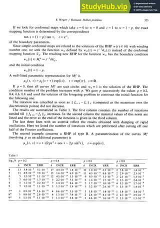
The interplay of the three branches influences the moment of stopping the iteration by the
above criterion. This is shown in Fig. 3 for N = 32 in dependence on p. Between p = 0.435 and
p = 0.438 the second branch of log 11 zyxwvutsrqponmlkjihgfedcbaZYXWVUTSRQPONMLKJIHGFEDCB
fk+i - fk 11
becomes horizontal and therefore the moment of
canceling the iteration is determined by the intersection of the first and the second branch for
p > 0.438, while the intersection of the second and the third branch is decisive if p < 0.435. This
explains the very steep descent in Fig. 3.
With regard to time saving, the above observations suggest to replace the criterion for
canceling the iteration by a refined one which detects the critical moment of going over to
linearly decreasing log 11
fk+1- fk 11.
Another way is to restrict the number of iterations, by 10,
say. This might be especially important if one intends to use the method as a black box in a
larger program. zyxwvutsrqponmlkjihgfedcbaZYXWVUTSRQPONMLKJIHGFEDCBA
Acknowledgement
I wish to thank the referee for his valuable remarks and hints, especially for those concerning
the convergence of the discrete method.
References
[l] M.H. Gutknecht, Fast algorithms for the conjugate periodic function, Computing 22 (1979) 79-91.
[2] M.H. Gutknecht, Numerical conformal mapping methods based on function conjugation, J. Comput. Appl. Math.
14 (1986) 31-77.
[3] J.W. Helton and R.E. Howe, A bang-bang theorem for optimization over spaces of analytic functions, J. Approx.
Theory 47 (1986) 101-121.
[4] P. Henrici, Apphed and Computational Complex Analysis, Vol. IZZ (Wiley, New York, 1986).
[5] 0. Htibner, The Newton method for solving the Theodorsen integral equation, J. Comput. Appl. Math. 14 (1986)
19-30.
[6] A.I. Snirel’man, A degree for quasi linear-like mapping and the nonlinear Hilbert problem (in Russian), Mat. Sb.
89 (113) (1972) 366-389.
[7] B.A. Vertgejm, Approximate construction of some conformal mappings (in Russian), Dokl. Akad. Nauk SSSR
119 (1958) 12-14.
[8] E. Wegert, Topological methods for strongly nonlinear Riemann-Hilbert problems for holomorphic functions,
Math. Nachr. 134 (1987) 201-230.
[9] E. Wegert, Boundary value problems and extremal problems for holomorphic functions, Complex Variables
Theory Appl., to appear.
[lo] E. Wegert and L. v. Wolfersdorf, Plane potential flow past a cylinder with porous surface, Math. Methods AppZ.
Sci. 9 (1987) 587-605.
[ll] R. Wegmann, Ein Iterationsverfahren zur konformen Abbildung, Numer. Math. 30 (1978) 453-466; translated as:
An iterative method for conformal mapping, J. Comput. Appl. Math. 14 (1986) 7-18.
[12] R. Wegmann, Convergence proofs and error estimates for an iterative method for conformal mapping, Numer.
Math. 44 (1984) 435-461.
[13] R. Wegmann, Discrete Riemann-Hilbert problems, interpolation of simply closed curves, and numerical
conformal mapping, J. Comput. Appl. Math. 23 (1988) 323-352.
[14] L. v. Wolfersdorf, Zur Unit% der Lijsung der Theodorsenschen Integralgleichung der konformen Abbildung, Z.
Anal. Anwendungen 3 (1984) 523-526.
[15] L. v. Wolfersdorf, Landesman-Lazer’s type boundary value problems for holomorphic functions, Math. Nachr.
114 (1983) 181-189.

An iterative method for solving nonlinear Riemann Hilbert problems.pdf

More Related Content

Similar to An iterative method for solving nonlinear Riemann Hilbert problems.pdf

More from Sarah Adams

Recently uploaded

An iterative method for solving nonlinear Riemann Hilbert problems.pdf