Downloaded 743 times

![2 The Dirichlet Problem in the Complex Plane
Cauchy-Riemann equations). In other words, a function satisfying of/oz == 0
may depend on z but not on z. Likewise, a function that satisfies af / 0 Z == 0
on a planar open set may depend on z but cannot depend on z.
Observe that
o
- z == 1
o
-z==O
oz oz
o o
- z ==0
oz ozz == 1.
Finally, the Laplacian is written in complex notation as
1.2 The Dirichlet Problem
Introductory Remarks
Throughout this book we use the notation C k (X) to denote the space of func-
tions that are k-times continuously differentiable on X-that is, functions that
possess all derivatives up to and including order k and such that all those
derivatives are continuous on X. When X is an open set, this notion is self-
explanatory. When X is an arbitrary set, it is rather complicated, but possible,
to obtain a complete understanding (see [STSI]).
For the purposes of this book, we need to understand the case when X is
a closed set in Euclidean space. In this circumstance we say that f is C k
on X if there is an open neighborhood U of X and a C k function j on U
1
such that the restriction of to X equals f. We write f E Ck(X). In case
k == 0, we write either CO(X) or C(X). This definition is equivalent to all
other reasonable definitions of C k for a non-open set. We shall present a more
detailed discussion of this matter in Section 3.
Now let us formulate the Dirichlet problem on the disc D. Let ¢ E C(oD).
The Dirichlet problem is to find a function U E C(D) n C 2 (D) such that
~U(z) == 0 if zED
U(z) == ¢ ( z) if z E aD.
REMARK Contrast the Dirichlet problem with the classical Cauchy problem
for the Lapiacian: Let S ~ lR2 == C be a smooth, non-self-intersecting curve](https://image.slidesharecdn.com/partialdifferentialequationsandcomplexanalysis-121120212851-phpapp02/85/Partial-differential-equations-and-complex-analysis-13-320.jpg)
![The Dirichlet Problem 3
s
u
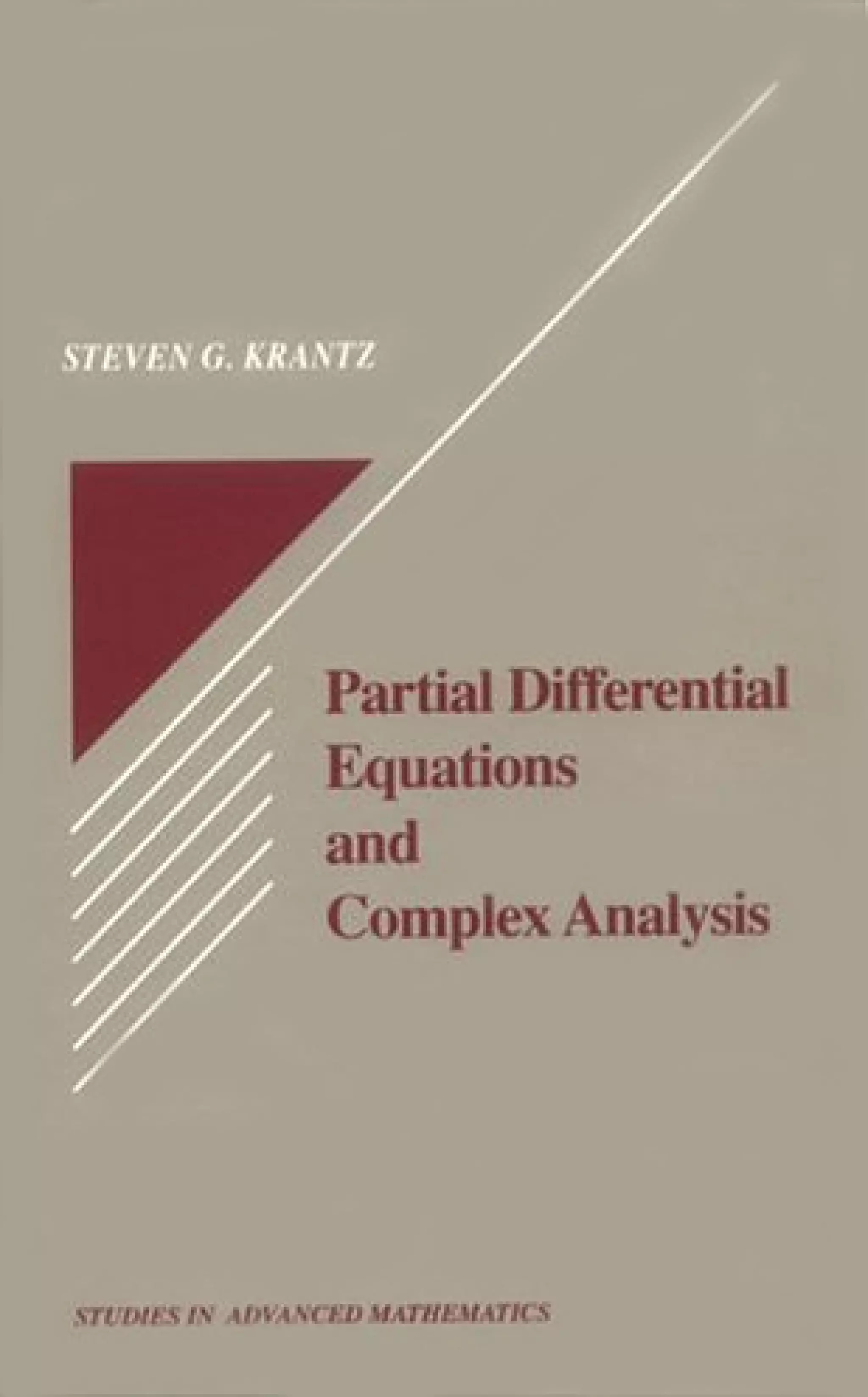
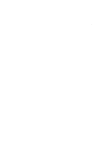
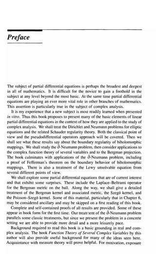
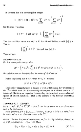
FIGURE 1.1
(part of the boundary of a smoothly bounded domain, for instance). Let U be
an open set with nontrivial intersection with S (see Figure 1.1). Finally, let ¢o
and ¢l be given continuous functions on S. The Cauchy problem is then
~u(z) == 0 if z E U
u(z) == ¢l (z) if z E S n U
au (z) == ¢l
av if z E S n U.
Here v denotes the unit normal direction at z E S.
Notice that the solution to the Dirichlet problem posed above is unique: if
Ul and U2 both solve the problem, then Ul - U2 is a hannonic function having
zero boundary values on D. The maximum principle thea implies that Ul == U2.
In particular, in the Dirichlet problem the specifying of boundary values also
uniquely determines the normal derivative of the solution function u.
However, in order to obtain uniqueness in the Cauchy problem, we must
specify both the value of U on S and the normal derivative of u on S. How can
this be? The reason is that the Dirichlet problem is posed with a simple closed
boundary curve; the Cauchy problem is instead a local one. Questions of when
function theory reflects (algebraic) topology are treated, for instance, by the de
Rham theorem and the Atiyah-Singer index theorem. We shall not treat them
in this book, but refer the reader to [GIL], [KRl], [DER]. I](https://image.slidesharecdn.com/partialdifferentialequationsandcomplexanalysis-121120212851-phpapp02/85/Partial-differential-equations-and-complex-analysis-14-320.jpg)
![The Dirichlet Problem 5
If we sum the two geometric series and do the necessary algebra then we find
that
27r 1 2
S 0 - -1
(r, ) - 21r 0
f it
1 - r d
( e ) 1 - 2r cos (0 - t) + r 2 t.
This last formula allows one to do the estimates to check for uniform conver-
gence, and thus to justify the change of order of the sum and the integral.
We set
=~
2
Pr ( 'lj;) 1- r
27r 1 - 2r cos ('l/J) + r2 '
and we call this function the Poisson kernel. Since the function
u(re iO ) == S(r, 0)
is the limit of the partial sums TN(r, 0) == E:=-N anrlnleinO, and since each
of the partial sums is hannonic, u is hannonic. Moreover, the partial sum
TN is the harmonic function that solves the Dirichlet problem for the data
f N(e iO ) == E:=_
N an einO . We might hope that u is then the solution of the
Dirichlet problem with data f. This is in fact true:
THEOREM 1.2.3
Let f(e it ) be a continuous function on aD. Then the function
u(reiO ) == { J~7r.f(ei(O-t))Pr(t) dt if 0 :::; r < 1
f(e~O) ifr == 1
solves the Dirichlet problem on the disc with data f.
PROOF Pick E > O. Choose 8 > 0 such that if Is - tl < 8, then If( eis ) -
f (e it )I < Eo Fix a point eiO E aD. We will first show that limr-t 1- u(re iO ) ==
f(e iO ) == u(e iO ). Now, for 0 < r < 1,
lu(re ill ) - I(e ill )/ = 11 2
71: l(e i(II-t»)Pr(t) dt - l(eill)l. (1.2.3.1)
Observe, using the sum from which we obtained the Poisson kernel, that
f27r f27r
1 IPr(t)1 dt = 1 Pr(t) dt = 1.
0 0
Thus we may rewrite (1.2.3.1) as
r
io
2
71: [I (e i(lI-t») - 1 (e ill )] Pr (t) dt =
i
r
1 tl<8
[I (e i(lI-t») - f( eill )] Pr (t) dt
+l<::,t <::'27r-JI( ei(lI-t») - I( eill )] Pr(t) dt
== I + II.](https://image.slidesharecdn.com/partialdifferentialequationsandcomplexanalysis-121120212851-phpapp02/85/Partial-differential-equations-and-complex-analysis-16-320.jpg)
![Lipschitz Spaces 7
1.3 Lipschitz Spaces
Our first aim in this book is to study the boundary regularity for the Dirich-
let problem: if the data f is "smooth," then will -the solution of the Dirichlet
problem be smooth up to the boundary? This is a venerable question in the
theory of partial differential equations and will be a recurring theme throughout
this book. In order to formulate the question precisely and give it a careful
answer, we need suitable function spaces.
The most naive function spaces for studying the question formulated in the
last paragraph are the C k spaces, mentioned earlier. However, these spaces
are not the most convenient for our study. The reason, which is of central
importance, is as follows: We shall learn later, by a method of Hormander
[H03], that the boundary regularity of the Dirichlet problem is equivalent to the
boundedness of certain singular integral operators (see [STSI]) on the boundary.
Singular integral operators, central to the understanding of many problems in
analysis, are not bounded on the C k spaces. (This fact explains the mysteriously
imprecise formulation of regularity results in many books on partial differential
equations. It also means that we shall have to work harder to get exact regularity
results.)
Because of the remarks in the preceding paragraph, we now introduce the scale
of Lipschitz spaces. They will be somewhat familiar, but there will be some
new twists to which the reader should pay careful attention. A comprehensive
study of these spaces appears in [KR2].
Now let U ~ ~N be an open set. Let 0 < Q < 1. A function f on U is said
to be Lipschitz of order Q, and we write f E An, if
If(x + h) - f(x)1
sup
h:;tO
Ihl a + Ilfllux,(u) == IlfIIA,,(U) < 00.
x,x+hEU
We include the term IIfIILoo(u) in this definition in order to guarantee that the
Lipschitz norm is a true norm (without this term, constant functions would have
"norm" zero and we would only have a semi-norm). In other contexts it is
useful to use IlfIlLP(u) rather than IlfIILOO(U). See [KR3] for a discussion of
these matters.
When Q == 1 the "first difference" definition of the space An makes sense,
and it describes an important class of functions. However, singular integral
operators are not bounded on this space. We set this space of functions apart
by denoting it differently:
sup If(x + h) - f(x)1
Ihl +
IIIII Loo(U) < 00.
h=¢.O
x,x+hEU](https://image.slidesharecdn.com/partialdifferentialequationsandcomplexanalysis-121120212851-phpapp02/85/Partial-differential-equations-and-complex-analysis-18-320.jpg)
![The Dirichlet Problem in the Complex Plane
The space Lipl is important in geometric applications (see [FED]), but less so
in the context of integral operators. Therefore we define
IIfIIA ==
If(x + h) + I(x - h) - 2/(x)1 IIIII
1 (U) sup
h:;iO
Ihl + LCXJ(U) < 00.
x,x+h,x-hEU
Inductively, if 0 < k E Z and k < a ::; k + 1, then we define a function f
on U to be in Aex if I is bounded, I E C1(U), and any first derivative Djl
lies in Aex - l . Equivalently, I E A ex if and only if f is bounded and, for every
nonnegative integer f < Q and multiindex {3 of total order not exceeding f we
have (8 j 8x)(3 I exists, is continuous, and lies in Aex - f .
The space Lip k' 1 < k E Z, is defined by induction in a similar fashion.
REMARK As an illustration of these ideas, observe that a function 9 is in
AS / 2(U) if 9 is bounded and the derivatives 8gj8xj, 82gj8xj8xk exist and lie
in A1/ 2 •
Prove as an exercise that if Q' > Q then Aexl ~ A ex . Also prove that the
Weierstrass nowhere-differentiable function
00
F(O) == L 2- e j i2ie
j=O
is in Al (0, 27r) but not in LiPl (0, 21r). Construct an analogous example, for
each positive integer k, of a function in A k Lip k'
If U is a bounded open set with smooth boundary and if 9 E Aex(U) then
does it follow that 9 extends to be in A ex (U)? I
Let us now discuss the definition of C k spaces in some detail. A function
f on an open set U ~ }RN is said to be k-times continuously differentiable,
written lEek (U), if all partial derivatives of I up to and including order k
exist on U and are continuous. On }Rl , the function I (x) == Ixllies in CO C 1•
Examples to show that the higher order Ok spaces are distinct may be obtained
by anti-differentiation. In fact, if we equip Ok (U) with the norm
IlfIICk(U) == IlfIIL(X)(U) + L II (~::) II
lal::;k Loo(U)
'
then elementary arguments show that C k + 1 (U) is contained in, but is nowhere
dense in, Ck(U).](https://image.slidesharecdn.com/partialdifferentialequationsandcomplexanalysis-121120212851-phpapp02/85/Partial-differential-equations-and-complex-analysis-19-320.jpg)
![Lipschitz Spaces 9
It is natural to suspect that if all the k th order pure derivatives (a/ax j )f f exist
and are bounded, 0 ::; /!, ::; k, then the function has all derivatives (including
mixed ones) of order not exceeding k and they are bounded. In fact Mityagin
and Semenov [MIS] showed this to be false in the strongest possible sense.
However, the analogous statement for Lipschitz spaces is true-see [KR2].
Now suppose that U is a bounded open set in ~N with smooth boundary. We
would like to talk about functions that are C k on U == U u au. There are three
ways to define this notion:
I. We say that a function f is in C k (0) if f and all its derivatives on U of
order not exceeding k extend continuously to (j.
II. We say that a function f is in C k (0) if there is an open neighborhood
W of 0 and a C k function F on W such that Flo == f.
III. We say that a function f is in Ck(U) if f E Ck(U) and for each Xo E au
and each multiindex Q such that IQ I ::; k the limit
ao:
lim
U3x----+xo
-a f(x)
xO:
exists.
We leave as an exercise for the reader to prove the equivalence of these
definitions. Begin by using the implicit function theorem to map U locally to a
boundary neighborhood of an upper half-space. See [HIR] for some help.
REMARK A basic regularity question for partial differential equations is as
follows: consider the Laplace equation
.6u == f.
If f E ;'0: (~N ), then where (Le. in what smoothness class) does the function u
live (at least locally)?
In many texts on partial differential equations, the question is posed as "If
f E C k(~N) then where does u live?" The answer is generally given as
"u E Cl~:2-f for any E > 0." Whenever a result in analysis is formulated in
this fashion, it is safe to assume that either the most powerful techniques are not
being used or (more typically) the results are being formulated in the language
of the incorrect spaces. In fact, the latter situation obtains here. If one uses
the Lipschitz spaces, then there is no t-order loss of regularity: f E Ao: (~N)
implies that u is locally in AO:+ 2 (IR N ). Sharp results may also be obtained by
using Sobolev spaces. We shall explore this matter in further detail as the book
develops. I](https://image.slidesharecdn.com/partialdifferentialequationsandcomplexanalysis-121120212851-phpapp02/85/Partial-differential-equations-and-complex-analysis-20-320.jpg)
![Boundary Regularity 13
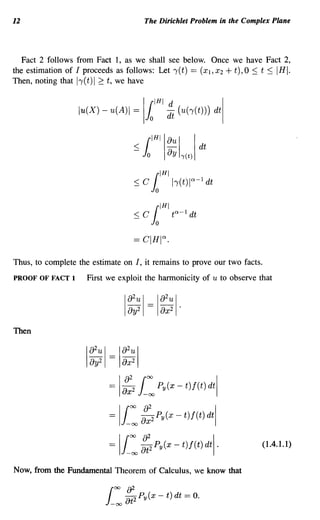
As a result, line (1.4.1.1) equals
Ii: ::2 Py (X - t) [J(t) - f(x)] dtl
< C i: ::2 I Py (X - t)llx - til> dt
cjOO 1
2Y (3(x - tf - ~2) IIX _ tl a dt
- 00 [ (x - t) 2 + y2]
2
C JOO Iy(3t - y2) Iit ia dt
-00 (t 2 + y2)3
OO 1
C a-2
y J -00 (t 2 + 1)2-a/2
dt
C ya-2 .
This completes the proof of Fact 1.
PROOF OF FACT 2 First notice that, for any x E IR,
:; ~1
7r -00
00
[(x - t)2 + y2]
2
I(x - tf + y - 22y21If(t)1 dtl
y=2
<~
- 7r
1
-00
00
If(t)1
(x - t)2 + y2
dtl
y=2
::; C . IIfIlLOO(~).](https://image.slidesharecdn.com/partialdifferentialequationsandcomplexanalysis-121120212851-phpapp02/85/Partial-differential-equations-and-complex-analysis-24-320.jpg)
![14 The Dirichlet Problem in the Complex Plane
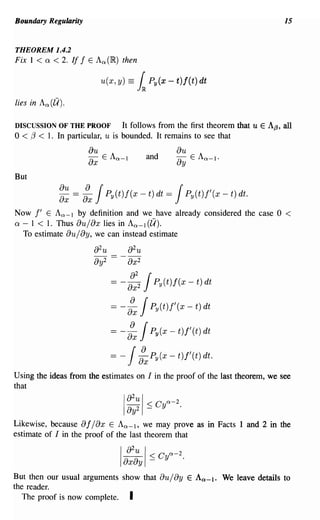
Now, if Yo ~ 2, then from Fact 1 we may calculate that
1~~(xO,Yo)1 ~ 11 ~:~(XO,Y)dY+ ~~(XO,2)1
YO
~ l YO
y"-2dy+ 1~~(XO,2)1
< Ca [ya-l
- 0 + 2a - l
] + C2
A nearly identical argument shows that
au( xo,yO) I ~
ay c 'a 1
Yo-
I
when 0 ::; Yo < 2.
We have proved Facts I and 2 and therefore have completed our estimates of
term I.
The estimate of I I I is just the same as the estimate for I and we shall say
no more about it.
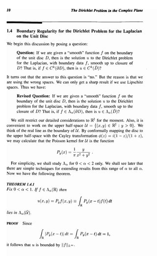
For the estimate of II, we write A == (aI, a2) and B == (b l , b2). Then
lu(A) - u(B)1 == lu(al' a2) - u(b l , b2)1
::; lu( aI, a2) - u(b l , a2) I + lu(b l , a2) - 'u(b l , b2) I
Assume for simplicity that al < bl as shown in Figure 1.2. Now set 7](t) =
(al + t, a2),O < t < bl - al. Then
bl - al d
I I I ==
l o
- (u 0 7]) (t) dt
dt
= Jo
rbl-al d
dt
1 00
-oc Pa2 (al + t - 8)f(8) d8 dt
I
I
bl-all°O -d Pa2(al + t -
d
==
l o -00 t
s) [f(s) - f(t)] ds dt.
We leave it as an exercise for the reader to see that this last expression, in
absolute value, does not exceed GIHla.
The tenn 112 is estimated in the same way that we estimated I. I](https://image.slidesharecdn.com/partialdifferentialequationsandcomplexanalysis-121120212851-phpapp02/85/Partial-differential-equations-and-complex-analysis-25-320.jpg)
![16 The Dirichlet Problem in the Complex Plane
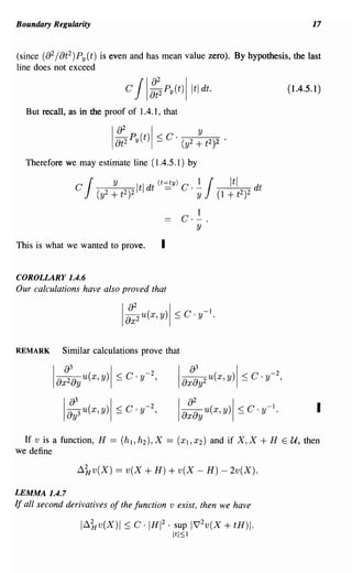
THEOREM 1.4.3
If f E AI(~), then
u(x, y) == l Py(x - t)f(t) dt
We break the proof up into a sequence of lemmas.
LEMMA 1.4.4
Fix y > O. Take (xo, YO) E U. Then
u(xo, Yo) = l Y
y' ()~~2 u(xo, Yo + y') dy' - y :y u(xo, Yo + y) + u(xo, y + Yo)·
PROOF Note that when y == 0, then the right-hand side equals O-O+u(xo, Yo).
Also, the partial derivative with respect to y of the right side is identically zero.
That completes the proof. I
LEMMA 1.4.5
If f E Al (~), then
PROOF Notice that, because u is harmonic,
I::2 ul = I::2 ul
=I ::2 f Py(x - t)f(t) dtl
= If (::2 Py(x - t)) f(t) dtl
= If (::2 Py(x - t)) f(t) dtl
= IJ (::2 Py(t)) f(x - t) dtl
= ~ IJ (:t: Py(t)) [I(x + t) + I(x - t) - 2f(x)] dtl](https://image.slidesharecdn.com/partialdifferentialequationsandcomplexanalysis-121120212851-phpapp02/85/Partial-differential-equations-and-complex-analysis-27-320.jpg)
![Boundary Regularity 19
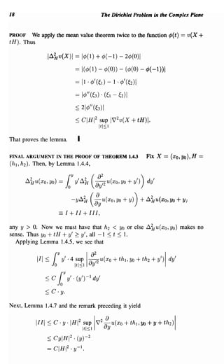
Finally, the same reasoning gives
11111::; IHI 2 . sup 1V'2 u (xo+th l ,yo+th2 +y)1
It I:::; I
::; C . IHI 2 . y-I.
Now we take y == 21HI. The estimates on 1,11,111 then combine to give
1~~u(X)1 ::; CIHI·
This is the desired estimate on u. I
REMARK We have proved that if f E Al (IR) then u == Pyf E Al (U) us-
ing the method of direct estimation. An often more convenient, and natural,
methodology is to use interpolation of operators, as seen in the next theorem.
I
THEOREM 1.4.8
Let V ~ IRm, W ~ IRn be open with smooth boundary. Fix 0 < 0: < (3
and assume that T is a linear operator such that T : Aa(V) ~ Aa(W) and
T : A{J(V) ~ A{J(W). Then, for all 0: < 1 < (3 we have T : A,(V) ~ A,(W).
Interpolation of operators, presented in the context of Lipschitz spaces, is
discussed in detail in [KR2]. The subject of interpolation is discussed in a
broader context in [STW] and [BOL]. Here is an application of the theorem:
Let 0: == 1/2, {3 == 3/2, and let T be the Poisson integral operator from
functions on IR to functions on U. We know that
and
We may conclude from the theorem that
Thus we have a neater way of seeing that Poisson integration is well behaved
on AI.
REMARK Twenty years ago it was an open question whether, if T is a bounded
linear operator on CO and on C 2 , it follows that T is a bounded linear operator
on C l . The answer to this question is negative; details may be found in [MIS].
In fact, AI is the appropriate space that is intennediate to CO and C2.](https://image.slidesharecdn.com/partialdifferentialequationsandcomplexanalysis-121120212851-phpapp02/85/Partial-differential-equations-and-complex-analysis-30-320.jpg)
![20 The Dirichlet Problem in the Complex Plane
One might ask how Poisson integration is behaved on Lip I (IR). Set f(x) ==
Ixl· ¢(x) where ¢ E Cgo(IR), ¢ == 1 near O. One may calculate that
(x, Y ) == P yf (x ) == ~ In [ (1 - 2x) + y2 . (1 +2x) + y2]
2 2
U 2- 2 2
X +y x +y
+x 1- x 1+ x]
[ arctan -y- - arctan -y-
+ (smooth error).
Set x == O. Then, for y small,
Again, we see that the classical space Lipi does not suit our purposes, while
Al does. We shall not encounter LiPI any more in this book. The space Al was
invented by Zygmund (see [ZYG]), who called it the space of smooth functions.
He denoted it by A*.
Here is what we have proved so far: if ¢ is a piece of Dirichlet data for
the disc that lies in An (aD), 0 < a < 2, then the solution u to the Dirichlet
problem with that data is An up to the boundary. We did this by transferring
the problem to the upper half-space by way of the Cayley transform and then
using explicit calculations with the Poisson kernel for the half-space.
1.5 Regularity of the Dirichlet Problem on a Smoothly Bounded
Domain and Conformal Mapping
We begin by giving a precise definition of a domain "with smooth boundary":
DEFINITION 1.5.1 Let U ~ C be a bounded domain. We say that U has
smooth boundary if the boundary consists of finitely many curves and each of
these is locally the graph of a COO function.
In practice it is more convenient to have a different definition of domain with
smooth boundary. A function p is called a defining function for U if p is defined
in a neighborhood W of au, l p i= 0 on au, and wnu == {z E W : p(z) < O}.
Now we say that U has smooth (or C k ) boundary if U has a defining function
p that is smooth (or C k ). Yet a third definition of smooth boundary is that the
boundary consists of finitely many curves rj, each of which is the trace of a
smooth curve r( t) with nonvanishing gradient. We invite the reader to verify
that these three definitions are equivalent.](https://image.slidesharecdn.com/partialdifferentialequationsandcomplexanalysis-121120212851-phpapp02/85/Partial-differential-equations-and-complex-analysis-31-320.jpg)
![Regularity of the Dirichlet Problem 21
"",---- ........... ,
/ ", "
/_-........" U ",
/-- ........
""
I / " / /
~ '
laD'
Iw /
I / ~ I
I I
I
aD
/ I I I
/ / I I /
I ( / / I
"
au' / / / ",/
"'-..... -. ' - _ / "'B /
"........
" ........ _--_/ ",
/
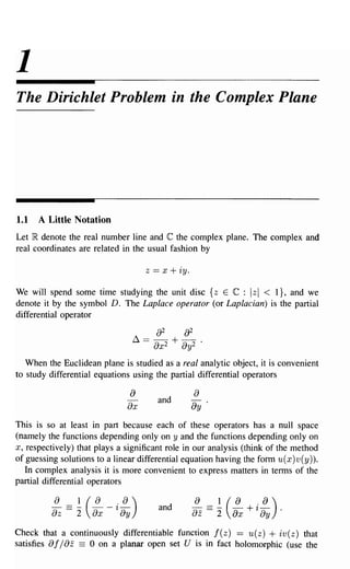
FIGURE 1.3
Our motivating question for the present section is as follows:
Let n ~ C be a bounded domain with smooth boundary. Assume
that! E An (an). If u E C(n) satisfies (i) u is harmonic on nand
(ii) ulan == !, then does it follow that u E An(n)?
Here is a scheme for answering this question:
Step 1: Suppose at first that U is bounded and simply connected.
Step 2: By the Riemann mapping theorem, there is a conformal mapping ¢ :
U ~ D. Here D is the unit disc. We would like to reduce our problem
to the Dirichlet problem on D for the data ! 0 ¢ - 1•
In order to carry out this program, we need to know that ¢ extends smoothly
to the boundary. It is a classical result of Caratheodory [CAR] that if a simply
connected domain U has boundary consisting of a Jordan curve, then any con-
formal map of the domain to the disc extends univalently and bicontinuously to
the boundary. It is less well known that Painleve, in his thesis [PAl], proved that
when U has smooth boundary then the conformal mapping extends smoothly to
the boundary. In fact, Painleve's result long precedes that of Caratheodory.
We shall present here a modem approach to smoothness to the boundary
for conformal mappings. These ideas come from [KERl]. See also [BKR]
for a self-contained approach to these matters. Our purpose here is to tie the
smoothness-to-the-boundary issue for mappings directly to the regularity theory
of the Dirichlet problem for the Laplacian.
Refer to Figure 1.3. Let W be a collared neighborhood of au. Set au' ==
aw n U and let aD' == ¢(aU'). Define B to be the region bounded by aD](https://image.slidesharecdn.com/partialdifferentialequationsandcomplexanalysis-121120212851-phpapp02/85/Partial-differential-equations-and-complex-analysis-32-320.jpg)
![22 The Dirichlet Problem in the Complex Plane
and aD'. We solve the Dirichlet problem on B with boundary data
I if (E aD
f(() ={ 0 if (E aD'.
Call the solution u.
Consider v == u 0 ¢ : U ~ nt Then, of course, v is still hannonic. By
Caratheodory's theorem, v extends to au, au', and
I if (E au
v == { 0 if (E au'.
Suppose that we knew that solutions of the Dirichlet problem on a smoothly
bounded domain with Coo data are in fact Coo on the closure of the domain.
Then, if we consider a first-order derivative V of v, we obtain
IVvl == IV(u 0 ¢)I == l7ull7¢1 ~ C.
It follows that
(1.5.2)
This will prove to be a useful estimate once we take advantage of the following
lemma.
LEMMA 1.5.3 HOPF'S LEMMA
Let n cc }RN have C 2 boundary. Let u E C(n) with u harmonic and noncon-
stant on n. Let PEn and assume that u takes a local minimum at P. Then
the one-sided normal derivative satisfies
au
av (P) < O.
PROOF Suppose without loss of generality that u > 0 on n near P and that
n
u(P) == O. Let B R be a ball that is internally tangent to at P. We may assume
that the center of this ball is at the origin and that P has coordinates (R, 0, ... ,0).
Then, by Harnack's inequality (see [KR1]), we have for 0 < r < R that
R2 - r 2
u(r, 0, ... , 0) ~ c· R2 + r 2 '
hence
u(r,O, ... ,O)-u(R,O, ... ,O) , 0
- - - - - - - - - - - < -c < .
r-R -
Therefore
ou() ,
ov p ~ -c < o.
This is the desired result. I](https://image.slidesharecdn.com/partialdifferentialequationsandcomplexanalysis-121120212851-phpapp02/85/Partial-differential-equations-and-complex-analysis-33-320.jpg)
![Regularity of the Dirichlet Problem 23
Now let us return to the u from the Dirichlet problem that we considered
prior to line (1.5.2). Hopf's lemma tells us that l7ul 2 c' > 0 near aD. Thus,
from (1.5.2), we conclude that
17¢1 ~ C. (1.5.4)
Thus we have bounds on the first derivatives of ¢.
To control the second derivatives, we calculate that
C 2 17 2 vl == 17(7v) 1== 17(7(u 0 ¢))I
== 1 (7 u ( ¢) . 7¢)1== 1(7 2U . [7¢] 2 ) + (7 u . 7 2 ¢)
7 I·
Here the reader should think of 7 as representing a generic first derivative and
72 a generic second derivative. We conclude that
Hence (again using Hopf's lemma),
17 2 "'1 <
f' -
~
l7ul
< C".
-
In the same fashion, we may prove that l7 k ¢1 ~ Ck , any k E {1,2, ...}. This
means (use the fundamental theorem of calculus) that ¢ E Coo (0).
We have amved at the following situation: Smoothness to the boundary
of confonnal maps implies regularity of the Dirichlet problem on a smoothly
bounded domain. Conversely, regularity of the Dirichlet problem can be used,
together with Hopf's lemma, to prove the smoothness to the boundary of con-
formal mappings. We must find a way out of this impasse.
Our solution to the problem posed in the last paragraph will be to study the
Dirichlet problem for a more general class of operators that is invariant under
smooth changes of coordinates. We will study these operators by (i) localizing
the problem and (ii) mapping the smooth domain under a diffeomorphism to
an upper half-space. It will tum out that elliptic operators are invariant under
these operations. We shall then use the calculus of pseudodifferential operators
to prove local boundary regularity for elliptic operators.
There is an important point implicit in our discussion that deserves to be
brought into the foreground. The Laplacian is invariant under conformal trans-
formations (exercise). This observation was useful in setting up the discussion
in the present section. But it turned out to be a point of view that is too narrow:
we found ourselves in a situation of circular reasoning. We shall thus expand
to a wider universe in which our operators are invariant under diffeomorphisms.
This type of invariance will give us more flexibility and more power.
Let us conclude this section by exploring how the Laplacian behaves under
a diffeomorphic change of coordinates. For simplicity, we restrict attention to](https://image.slidesharecdn.com/partialdifferentialequationsandcomplexanalysis-121120212851-phpapp02/85/Partial-differential-equations-and-complex-analysis-34-320.jpg)
![24 The Dirichlet Problem in the Complex Plane
]R2 with coordinates (x, y). Let
¢ ( x, y) == (¢ 1 (x, y), cP2 (x, y)) == (x', y')
be a diffeomorphism of }R2. Let
In (x', y') coordinates, the operator ~ becomes
In an effort to see what the new operator has in common with the old one, we
introduce the notation
where
a a a a
axO: axr 1 ax~2 ... ax~n
is a differential monomial. Its "symbol" (for more on this, see the next two
chapters) is defined to be
The symbol of the Laplacian ~ == (a 2 / ax 2 ) + (a 2 / ay2) is
(J(~) == ~f + ~i·
Now associate to (J(~) a matrix ..4~ == (aij)1:S;i,j:S;2, where aij = aij(x) is the
coefficient of ~i~j in the symbol. Thus
The symbol of the transfonned Laplacian (in the new coordinates) is
(J(¢*(~)) == 17¢112~f + 17¢212~i
ax' ay' ax' ay,]
+2 [ - - + - - ~le2
ax ay By By
+ (lower order tenns).](https://image.slidesharecdn.com/partialdifferentialequationsandcomplexanalysis-121120212851-phpapp02/85/Partial-differential-equations-and-complex-analysis-35-320.jpg)
![2
Review of Fourier Analysis
2.1 The Fourier Transform
A thorough treatment of Fourier analysis in Euclidean space may be found in
[STW] or [HOR4]. Here we give a sketch of the theory.
If t, ~ E }RN then we let
t· ~ == tl~1 + ... + tN~N.
We define the Fourier transform of an f E £1 (I~N) by
j(~) = Jf(t)eit.~ dt.
Many references will insert a factor of 271" in the exponential or in the measure.
Others will insert a minus sign in the exponent. There is no agreement on this
matter. We have opted for this definition because of its simplicity. We note that
the significance of the exponentials eit.~ is that the only continuous multiplicative
homomorphisms of}RN into the circle group are the functions ¢~ (t) == eit.~.
(We leave this as an exercise for the reader. A thorough discussion appears
in [KAT] or [BAC].) These functions are called the characters of the additive
group }RN.
Basic Properties of the Fourier Transform
PROPOSITION 2.1.1
If f E £1 (}RN) then
PROOF Observe that
Ij(~) I ::; J If(t)1 dt. I](https://image.slidesharecdn.com/partialdifferentialequationsandcomplexanalysis-121120212851-phpapp02/85/Partial-differential-equations-and-complex-analysis-37-320.jpg)
 J (pf)(t)eif,.t dt = J f(p(t))eif,.t dt
(s=g,(t)) J f(s)e i f,.p-'(s) ds =J f(s)eip(f,).s ds
(p(j)) (~). I
PROPOSITION 2.1.8
We have
PROOF We calculate that
PROPOSITION 2.1.9
If 8 > 0 and f E L 1(IR N ), then we set 08f(x)
8- N f(x/8). Then
(alif) = ali (I)
0 8f == 08j.
PROOF We calculate that
(alif) = J(ali/) (t)eit.f, dt = J f(8t)e it .f, dt
= J f(t) ei(t/li)-f, 8- N dt = 8- N j(E,/8) = ali(j).
That proves the first assertion. The proof of the second is similar. I
If I, g are L 1 functions, then we define their convolution to be the function
f * g(x) = J f(x - t)g(t) dt = J g(x - t)f(t) dt.
It is a standard result of measure theory (see [RUD3]) that I *g so defined is
an L 1 function and III * gllL1 ::; IIfllL1 IIgllLI.](https://image.slidesharecdn.com/partialdifferentialequationsandcomplexanalysis-121120212851-phpapp02/85/Partial-differential-equations-and-complex-analysis-40-320.jpg)
![The Fourier Transform 31
PROOF It is enough to do the case N == 1. Set I == J~oo e- t2 dt. Then
I "I = I: I: e-
s2
ds e-
t2
dt = II
IR2
e-!(s,t)!2 dsdt
{21r roo _r 2
= Jo Jo e rdrd()=7L
Thus I == ~, as desired. I
REMARK Although this is the most common method for evaluating J e- 1x !2 dx,
several other approaches are provided in [HEI]. I
Now let us calculate the Fourier transform of e- 1xI2 • It suffices to treat the
one-dimensional case because
(e- 1xI2 f = IN e-lx!2eixof, dx = l e-x~eixlf,1 dX"""l e-x~eixNf,N dXN"
Now when N == 1 we have
l e-
x2 ix
+ f, dx =l e(f,/2+ix)2 e-e/ 4 dx
= e-e /4l e(f,/2+ix)2 dx
== e-~2 /4 { e(~/2+ix/2)2 ~ dx
J
IR 2
== ~e-~2 /4 1 e(Z/2)2 dz. (2.1.12.1)
2 Jr
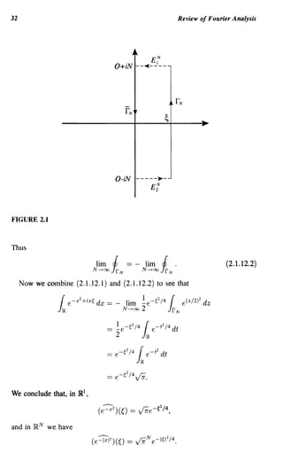
Here, for ~ E R fixed, r == r ~ is the curve t ~ ~ + it. Let r N be the part of
the curve between t == - Nand t == N. Since Ir
== limN ---l>OO Jr N' it is enough
J
for us to understand r N' Refer to Figure 2.1.
Now
Therefore
But, as N -+ 00,
1 +1 -+ O.
JEfl JEr](https://image.slidesharecdn.com/partialdifferentialequationsandcomplexanalysis-121120212851-phpapp02/85/Partial-differential-equations-and-complex-analysis-42-320.jpg)
![The Fourier Transform 33
It is often convenient to scale this formula and write
The function G(x) == (27r)-N/2 e- 1 I2 /2 is called the Gauss-Weierstrass ker-
x
nel. It is a summability kernel (see [KAT]) for the Fourier transform. Observe
that G(~) == e-I~12 /2.
On R N we define
Then
-- --
~(~) = (e-'1~12 /2) = (avee-I~12 /2)
= ave [(27r)N/2e-I~12/2]
== E-N/2(27r)N/2e-I~12 /(2E).
Now assume that !, j are in L 1 and are continuous. We apply Proposi-
tion 2.1.11 with 9 == GE ELI. We obtain
Jf~(x) Jj(~)C.(~) d~.
dx =
In other words,
(2.1.13)
Now e-EI~12 /2 - t 1 uniformly on compact sets. Thus J j(~)e-EI~12 d~ -t
J j(~) d~. That takes care of the right-hand side of (2.1.13).
Next observe that
Thus the left side of (2.1.13) equals
(27r)N Jf(x)G,(x) dx = (27r)N J f(O)G,(x) dx
+(27r)N j[f(x) - f(O)JG,(x) dx
-t (27r)N ·1(0).](https://image.slidesharecdn.com/partialdifferentialequationsandcomplexanalysis-121120212851-phpapp02/85/Partial-differential-equations-and-complex-analysis-44-320.jpg)
![34 Review of Fourier Analysis
Thus we have evaluated the limits of the left- and right-hand sides of (2.1.13).
We have proved the following theorem.
THEOREM 2.1.14 THE FOURIER INVERSION FORMULA
If !, j E £1 and both are continuous, then
f(O) = (27r)-N Jj(~) d~. (2.1.14.1 )
Of course there is nothing special about the point 0 E R N . We now exploit
the compatibility of the Fourier transform with translations to obtain a more
general formula. First, we define
(Th!)(x) == I(x - h)
for any function I on RN and any h E RN . Then, by a change of variable in
the integral,
T;] == eih.~ j(~).
Now we apply formula (2.1.14.1) in our theorem to T-h/: The result is
or
THEOREM 2.1.15
If I, j E £1 then for any h E R N we have
f(h) = (2JT)-N Jj(~)e-ih.f, d~.
COROLLARY 2.1.16
The Fourier transform is univalent. That is, if I, 9 E £1 and j == 9 then f = 9
almost everywhere.
PROOF Since I - 9 E £1 and j - g == 0 E £1, this is immediate from either
the theorem or (2.1.13). I
Since the Fourier transform is univalent, it is natural to ask whether it is
surjective. We have
PROPOSITION 2.1.17
The operator
is not onto.](https://image.slidesharecdn.com/partialdifferentialequationsandcomplexanalysis-121120212851-phpapp02/85/Partial-differential-equations-and-complex-analysis-45-320.jpg)
![The Fourier Transform 35
PROOF Seeking a contradiction, we suppose that the operator is in fact surjec-
tive. Then the open mapping principle guarantees that there is a constant C > 0
such that
IIIIILI :S cllj"L~'
On IR , let g(~) be the characteristic function of the interval [-1, 1]. The in-
I
verse Fourier transform of g is a nonintegrable function. But then {G 1/ j * g}
forms a sequence that is bounded in supremum norm but whose inverse Fourier
transforms are unbounded in £1 norm. That gives the desired contradiction.
I
Plancherel's Formula
PROPOSITION 2.1.18 PLANCHEREL
If I E C~ (IR N ) then
JIj(~)12 d~ = J (21T)N If(xW dx.
PROOF Define g( x) == I * 1E c~ (IRN ). Then
,,~ ,,~ ,,~ .... 2
9 == I . I == I . I == I . f == III . (2.1.18.1)
Now
g(O) = f * 1(0) = J f( -t)!( -t) dt = J f(t)/(t) dt = J 2
If(t)1 dt.
By Fourier inversion and formula (2.1.18.1) we may now conclude that
J If(t)1 2 dt = g(O) = (21T)-N Jg(~) d~ = (27T)-N JIj(~)12 df
That is the desired formula. I
COROLLARY 2.1.19
If f E £2 (IR N ) then the Fourier transform of I can be defined in the following
fashion: Let Ij E C~ satisfy fj -+ I in the £2 topology. It follows from
the proposition that {.fj } is Cauchy in £2. Let g be the £2 limit of this latter
sequence. We set j == g.
It is easy to check that the definition of j given in the corollary is independent
of the choice of sequence Ij E C~ and that
J11(01 d~ 2
= (21T)N J If(xW dx.](https://image.slidesharecdn.com/partialdifferentialequationsandcomplexanalysis-121120212851-phpapp02/85/Partial-differential-equations-and-complex-analysis-46-320.jpg)
![36 Review of Fourier Analysis
We now know that the Fourier transform F has the following mapping prop-
erties:
F: £1 ~ LX
F: L 2 ~ £2.
The Riesz-Thorin interpolation theorem (see [STW]) now allows us to conclude
that
F : £P ~ LP' , 1 ~ p ~ 2,
where p' == p/ (p - 1). If p > 2 then F does not map LP into any nice function
space. The precise norm of F on LP has been computed by Beckner [BEC].
Exercises: Restrict attention to dimension 1. Consider the Fourier transform F
as a bounded linear operator on the Hilbert space £2 (IR N ). Prove that the four
roots of unity (suitably scaled) are eigenvalues of F.
Prove that if p(x) is a Hermite polynomial (see [STW], [WHW]), then the
function p(x)e-lxI2/2 is an eigenfunction of F. (Hint: (ix!) == (j)' and == l'
-i~j.)
2.2 Schwartz Distributions
Thorough treatments of distribution theory may be found in [SCH], [HOR4],
[TRE2]. Here we give a quick review.
We define the space of Schwartz functions:
s = {¢ E c oo (IRN ) : Pa,(3(¢) == x~~ Ix
a
(~) (3 ¢(x) I < 00,
0: = (0:1, .. " O:N), {3 = ({31,"" (3N) }.
Observe that e- 1x12 E Sand p(x) . e- 1x12 E S for any polynomial p. Any
derivative of a Schwartz function is still a Schwartz function. The Schwartz
space is obviously a linear space.
It is worth noting that the space of Coo functions with compact support (which
we have been denoting by C~) forms a proper subspace of S. Since as recently
as 1930 there was some doubt as to whether C~ functions are genuine functions
(see [OSG]), it may be worth seeing how to construct elements of this space.
Let the dimension N equal 1. Define
if x ~ 0
if x < o.](https://image.slidesharecdn.com/partialdifferentialequationsandcomplexanalysis-121120212851-phpapp02/85/Partial-differential-equations-and-complex-analysis-47-320.jpg)
![Schwartz Distributions 37
Then one checks, using l'Hopital's Rule, that A E Coo (IR). Set
h(x) == A( -x - 1) . A(X + 1) E C~(I~).
I:
Moreover, if we define
g(x) = h(t) dt,
then the function
f(x) == g(x + 2) . g( -x - 2)
lies in C~ and is identically equal to a constant on (-1, 1). Thus we have
constructed a standard "cutoff function" on ~l. On IR N , the function
plays a similar role. '
Exercise: [The Coo Urysohn lemma] Let K and L be disjoint closed sets
in IR N . Prove that there is a Coo function ¢ on IR N such that ¢ == 0 on K and
¢ == 1 on L. (Details of this sort of construction may be found in [HIR].)
The Topology of the Space 5
The functions Pn,(3 are seminorms on 5. A neighborhood basis of 0 for the
corresponding topology on 5 is given by the sets
NE,f,m == {¢: L lal:S€
Pa,(3(¢) < E} .
1.6I:Sm
Exercise: The space 5 cannot be normed.
DEFINITION 2.2.1 A Schwartz distribution Q is a continuous linear functional
on 5. We write Q E 5'.
Examples:
1. If f EL I , then f induces a Schwartz distribution as follows:
S:3 qH--> f </>fdx E C.
We see that this functional is continuous by noticing that
If </>(x)f(x) dxl ::; sup 1</>1· Ilfll£l = C . Po,o(</».](https://image.slidesharecdn.com/partialdifferentialequationsandcomplexanalysis-121120212851-phpapp02/85/Partial-differential-equations-and-complex-analysis-48-320.jpg)
![38 Review of Fourier Analysis
A similar argument shows that any finite Borel measure induces a distri-
bution.
2. Differentiation is a distribution: On R I , for example, we have
5 ::1 ¢ ~ ¢'(O)
satisfies
I¢' (0) 1 ::; sup I¢' (x) I == PO.I (¢).
xElR
3. If f E LP (RN ), 1 :::; p ::; 00, then f induces a distribution:
Tf : S 3 </J f--> J </Jf dx E c.
To see that this functional is bounded, we first notice that
(2.2.2)
where 1/ p + 1/ p' == 1. Now notice that
(1 + Ix IN +I) I¢(x )I ::; C (po,o (¢) + PN + 1,0 ( ¢)) ,
hence
C
I</J(x) I ::; 1 + Ixl N +1 (Po,o( </J) + PN+I,O(</J)) .
Finally,
II</JII Lp f ::; c· [
J(1 + I~IN+I ) P
,
dx
] lip'
. [Po,o(</J) + PN+I,O(</J)] .
As a result, (2.2.2) tells us that
T f ( ¢) ::; ell f II Lp (Po ,0 ( ¢) + PN + I ,0 ( ¢)) .
Algebraic Properties of Distributions
(i) If Q, (3 E 5' then Q+ (3 is defined by (Q + (3) (¢) == Q(¢) + (3( ¢). Clearly
Q + (3 so defined is a Schwartz distribution.
(ii) If Q E 5' and C E C then CQ is defined by (CQ)(¢) == c[Q(¢)]. We see
that CQ E 5'.
(iii) If 1/J E 5 and Q E 5' then define (1/JQ) (¢) == Q(1/J¢). It follows that 1/JQ
is a distribution.
(iv) It is a theorem of Laurent Schwartz (see [SCH]) that there is no contin-
uous operation of multiplication on S'. However, it is a matter of great
interest, especially to mathematical physicists, to have such an operation.](https://image.slidesharecdn.com/partialdifferentialequationsandcomplexanalysis-121120212851-phpapp02/85/Partial-differential-equations-and-complex-analysis-49-320.jpg)
![Schwartz Distributions 39
Colombeau [CMB] has developed a substitute operation. We shall say no
more about it here.
(v) Schwartz distributions may be differentiated as follows: If J-l E S' then
(8/ 8x)(3 J-l E S' is defined, for ¢ E S, by
Observe that in case the distribution J-l is induced by integration against a
C~ function f, then the definition is compatible with what integration by
parts would yield.
Let us differentiate the distribution induced by integration against the function
f(x) == Ixl on lIt Now, for ¢ E S,
f'(¢) == - f(¢')
= - [ : f¢' dx
= -100 f(x)¢'(x) dx - [°00 f(x)¢'(x) dx
= _ roo x¢'(x) dx + fO x¢'(x) dx
io -00
00
=- [x¢(x)]: + 1 ¢(x) dx + [x¢(x)]~oo - [°00 ¢(x) dx
= roo ¢(x) dx _ fO ¢(x) dx.
io -00
Thus f' consists of integration against b( x) == -x (-00,0] + X[O,oo). This function
is often called the Heaviside function.
Exercise: Let n ~
R N be a smoothly bounded domain. Let v be the unit
outward normal vector field to 8n. Prove that -VXn E S'. (Hint: Use Green's
theorem. It will tum out that (- VXn) (¢) == Jan ¢ da, where da is area measure
on the boundary.)
The Fourier Transform
The principal importance of the Schwartz distributions as opposed to other dis-
tribution theories (more on those below) is that they are well behaved under the
Fourier transform. First we need a lemma:](https://image.slidesharecdn.com/partialdifferentialequationsandcomplexanalysis-121120212851-phpapp02/85/Partial-differential-equations-and-complex-analysis-50-320.jpg)
![42 Review of Fourier Analysis
THEOREM 2.2.6 STRUCTURE THEOREM FOR V'
flu E V' then
k
U == LDjJ-lj,
j=1
where J-lj is a finite Borel measure and each Dj is a differential monomial.
IDEA OF PROOF For simplicity, restrict attention to R I . We know that the
dual of the continuous functions with compact support is the space of finite
Borel measures. In a natural fashion, the space of C I functions with compact
support can be identified with a subspace of the set of ordered pairs of Ce
functions: f +-+ (I, f'). Then every functional on C~ extends, by the Hahn-
Banach theorem, to a functional on C e x C e . But such a functional will be
given by a pair of measures. Combining this information with the definition
of derivative of a distribution gives that an element of the dual of C~ is of the
form J-l1 + (J-l2)'. In a similar fashion, one can prove that an element of the dual
of C~ must have the form J-li + (J-l2)' + ... + (J-lk+I)(k).
Finally, it is necessary to note that V' is nothing other than the countable
union of the dual spaces (C~)'. I
The theorem makes explicit the fact that an element of V' can depend on
only finitely many derivatives of the testing function-that is, on finitely many
of the norms Pn,(3.
We have already noted that the Schwartz distributions are the most convenient
for Fourier transform theory. But the space V' is often more convenient in the
theory of partial differential equations (because of the control on the support
of testing functions). It will sometimes be necessary to pass back and forth
between the two theories. In any given context, no confusion should result.
Exercise: Use the Paley-Wiener theorem (discussed in Section 4) or some other
technique to prove that if cP E V then ¢ (j. V. (This fact is often referred to as
the Heisenberg uncertainty principle. In fact, it has a number of qualitative and
quantitative formulations that are useful in quantum mechanics. See [FEG] for
more on these matters.)
More on the Topology of V and V'
We say that a sequence {cPj} ~ V converges to ¢ E V if
1. all the functions ¢j have compact support in a single compact set K o;
2. PK,n(¢j - ¢) -+ 0 for each compact set K and for every multiindex Q.
I
The enemy here is the example of the "gliding hump": On R , if 'ljJ is a
fixed Coo function and ¢j (x) == 'ljJ (x - j), then we do not want to say that the
sequence {¢j} converges to O.](https://image.slidesharecdn.com/partialdifferentialequationsandcomplexanalysis-121120212851-phpapp02/85/Partial-differential-equations-and-complex-analysis-53-320.jpg)
![44 Review of Fourier Analysis
PROOF We calculate that
(a * g)(cP) = a(§ * cP) = aX [1 §(x - t)cP(t) dt] .
Here the superscript on Q denotes the variable in which Q is acting. This last
Next we introduce the concept of Friedrichs mollifiers. Let ¢ E C~ be
supported in the ball B (0, 1). For convenience we assume that ¢ 2: 0, although
this is not crucial to the theory. Assume that J ¢( x) dx == 1. Set ¢E (x) ==
N
E- ¢(x/ E).
The family {¢E} will be called a family of Friedrichs mollifiers in honor of
K. O. Friedrichs. The use of such families to approximate a given function
by smooth functions has become a pervasive technique in modem analysis. In
functional analysis, such a family is sometimes called a weak approximation to
the identity (for reasons that we are about to see). Observe that J ¢E (x) dx == 1
for every E > O.
LEMMA 2.3.3
If f E LP(RN ), 1~p ~ 00, then
PROOF The case p == 00 is obvious, so we shall assume that 1 :::; p < 00.
Then we may apply Jensen's inequality, with the unit mass measure ¢E(X) dx,
to see that
Ilf*cP,II1p = 111 P
f(x-t)cP,(t)dtI dx
:=; 1
1 If(x - t)IPlcP,(t)1 dt dx
= 11 If(x - t)IP dx cP,(t) dt
= 1IlflltpcP,(t) dt
== 11111~p· I
REMARK The function IE == f * ¢E is certainly Coo Gust differentiate under
the integral sign) but it is generally not compactly supported unless I is. I](https://image.slidesharecdn.com/partialdifferentialequationsandcomplexanalysis-121120212851-phpapp02/85/Partial-differential-equations-and-complex-analysis-55-320.jpg)
![Convolution and Friedrichs Mollijiers 45
LEMMA 2.3.4
For 1 :::; p < 00 we have
PROOF We will use the following claim: For 1 :::; p < 00 we have
where 7ft f (x) == ! (x - h). Assume the claim for the moment.
Now
II!< - !11~p 111 !(x - t)¢«t) dt - 1!(x)¢«t) dtl[
111[!(x - t) - f(x)]¢«t) dtl[
111[Ttf(x) - f(x)]¢«t) dtl[
< 1IITt! - fll~p¢«t) dt
(t=J-U)
== 1II -! liP ()
TJi,E! LP¢ J-l dJ-l.
In the inequality here we have used Jensen's inequality. Now the claim and the
Lebesgue dominated convergence theorem yield that lifE - fllLP -+ O.
To prove the claim, first observe that if 1/J E GYe then I Th1/J - 1/J I sup -+ 0
by uniform continuity. It follows that II Th 1/J - 1/J II Lp -+ O. Now if ! E LP is
arbitrary and E > 0, then choose 1/J E Ce such that II! - 1/J II Lp < E/2. Then
lim sup II Thf - !IILP :::; lim sup II Th(! -1/J)IILP + lim sup IITh1/J -1/JII :::; E.
h---+O h---+O h---+O
Since E > 0 was arbitrary, the claim follows. I
LEMMA 2.3.5
If ! E C e then fE -+ ! uniformly.
PROOF Let 1] > 0 and choose E > 0 such that if Ix-yl < E then If(x)- f(y)1 <
1]. Then
If«x) - !(x)1 11 f(x - t)¢«t) dt - !(x)1
=
= I/[f(x - t) - f(x)J¢«t) dtl](https://image.slidesharecdn.com/partialdifferentialequationsandcomplexanalysis-121120212851-phpapp02/85/Partial-differential-equations-and-complex-analysis-56-320.jpg)
![46 Review of Fourier Analysis
:; r J1tl$.E
Ij(x-t)-j(x)I¢«t)dt
::; / ry¢< (t) dt
== 1].
That completes the proof. I
Exercise: Is the last lemma true for a broader class of /? Prove that if
f E C~(IRN), then lifE - flick - t O.
Now if Q E V' and cPE is a family of Fredrichs mollifiers, then we define
o:«x) == 0: * cP«x) = o:(¢«x - .)) = 0: ('L:i<) .
LEMMA 2.3.6
Each QE is a Coo function. Moreover, Q E -t Q in the topology of V'.
PROOF For simplicity of notation, we restrict attention to dimension one. First
let us see that Q E is differentiable on R We calculate:
Q[cPE(X + h - .)] - Q[cPE(X - .)]
h
= 0: ( ¢< (x +h -1- cP< (x - .)) . (2.3.6.1)
Observe that
cP«x + h -1- ¢«x - .) _ ¢:(x _ .)
in the topology of V. Thus (2.3.6.1) implies that
0:< (x + h~ - o:«x) _ o:(cP:(x _ .))
as h - t O.
Now let us verify the convergence of Q E to Q. Fix a testing function 'l/J E V.
Then
0:< ( 'ljJ) = / 0:< ( x) 'ljJ (x) dx = / 0:
8
(cP< (x - s)) 'ljJ (x) dx
= 0:
8
[/ (¢«x - s)) 'ljJ(x) dX] = 0: 8
[/ (¢«x)) 'ljJ(x + s) dX]
= 0:
8
[/ ¢< ( -x )'ljJ( S - x) dX] . (2.3.6.2)](https://image.slidesharecdn.com/partialdifferentialequationsandcomplexanalysis-121120212851-phpapp02/85/Partial-differential-equations-and-complex-analysis-57-320.jpg)
![48 Review of Fourier Analysis
To see this, let ¢ E V. Then
REMARK If a E V' is compactly supported and 'l/J E £, then we can define
Q( 'l/J) in the following manner: Let supp Q ~ K a compact set. Let <I> E C~
be identically equal to 1 on K. Then we set Q ( 'l/J) == Q (<I> . 'l/J). I
Now let us use (2.3.8) to see that & is Coo when Q E V' is compactly
supported. For simplicity, we assume that the dimension is one. Then
Notice that we may pass the limit inside the brackets because the Newton quo-
tients converge in C k for every k on the support of Q. Thus we have shown
that & is differentiable. Iteration of this argument shows that & is Coo. We
shall learn in the next section that, in fact, the Fourier transform of a compactly
supported distribution is real analytic.
We conclude with a remark on how to identify a smooth distribution. The
spirit of this remark will be a recurring theme throughout this book. We ac-
complish this identification by examining the decay of & at infinity. Namely, let
¢ E C~ be such that ¢ == 1 on a large compact set. We write & == ¢& +(1- ¢ )&.
Applying the inverse Fourier transform (denoted by ---), we see that
Then, since (¢&) is compactly supported, the first term is a Coo function. We
conclude that, in order to see whether Q is Coo, we must examine (( 1 - ¢) &)".
But this says, in effect, that we must examine the behavior of & at infinity.
2.4 The Paley-Wiener Theorem
We begin by examining the so-called Fourier-Laplace transform. If f E C~ (I~N )
and ( == ~ + if] E ]RN + ilRN ~ eN, then we define
j(() = r
J~N
!(x)e ix -( dx.](https://image.slidesharecdn.com/partialdifferentialequationsandcomplexanalysis-121120212851-phpapp02/85/Partial-differential-equations-and-complex-analysis-59-320.jpg)
![leVleW oJ ~"ourier Analysis
for some C, K. As a result,
I&(()I == IQX(eix'()1 == IQx (¢((x))1
:S C L sup IDJ3¢(1
1J3I~K B(O,A)
:S C(I(I + I)K sup le ix .( I
xEB(O,A)
Next let us assume that Q is a C~ function supported in B(O, A). We shall
prove (2.4.1.2). Now
I&(()I = If a(x)e ix -<: dxl
::: r la(x)leA11m(1 dx
JB(O,A)
:S IIQIILle A1Im (l.
This is (2.4.1.2) with K == 0. To obtain (2.4.1.2) with K == 1 we write, for
(j i= 0,
I&(()I = If a(x)e
ix
-<: dxl
== Ifa(x)~~eix,(
Z(j aXj
dxl
= I :j f (&~j a(x)) eix .( dxl
:S _1 II~QII eA11m(l.
I(jl aXj Ll
We can iterate this argument to obtain (2.4.1.2) for every K.
Next we prove that if (2.4.1.2) holds then Q is a C~ function with support
in B(O, A). We write
la(x)1 = I(27r)-N f U(~)e-ix,~ d~1
= I(27r)-N JU(~ + i1])e-ix.(~+i'7) d~l·](https://image.slidesharecdn.com/partialdifferentialequationsandcomplexanalysis-121120212851-phpapp02/85/Partial-differential-equations-and-complex-analysis-61-320.jpg)
![Introduction to Pseudodifferential Operators 53
Ehrenpreiss and Malgrange, among others. The approach of Ehrenpreiss was to
write
u(x) = c· Ju(~)e-ix.~ d~ = J-1;1 j(~)e-ix,~ ~. 2
Using Cauchy theory, he was able to relate this last integral to
J- + I~
1.
~1712
j(~ + i1])e- ix '(U i7]) d~.
In this way he avoided the singularity at ~ == 0 of the right-hand side of (3.1.2).
Malgrange's method, by contrast, was to first study (3.1.1) for those f such
that j vanishes to some finite order at 0 and then to apply some functional
analysis.
We have already noticed that, for the study of Coo regularity, the behavior
of the Fourier transform on the finite part of space is of no interest. Thus
the philosophy of pseudodifferential operator theory is to replace the Fourier
multiplier 1/1~12 by the multiplier (1 - ¢(~))/1~12, where ¢ E C~(IRN) is
identically equal to 1 near the origin. Thus we define
for any 9 E C~. Equivalently,
Now we look at u - Pf, where f is the function on the right of (3.1.1):
.-..
(u - P f) == it - P f
1 A 1- ¢(~) A
=-~f+ 1~12 f
== _ ¢(~) fA
1~12 .
Then u - P f is a distribution whose Fourier transform has compact support,
that is, u - P f is Coo. So studying the regularity of u is equivalent to studying
the regularity of P f. This is precisely what we mean when we say that P is a
parametrix for the partial differential operator~. And the point is that P has
symbol - (1 - ¢) / 1~12, which is free of singularities.
Now let L be a partial differential operator with (smooth) variable coefficients:
The classical approach to studying such operators was to reduce to the constant](https://image.slidesharecdn.com/partialdifferentialequationsandcomplexanalysis-121120212851-phpapp02/85/Partial-differential-equations-and-complex-analysis-64-320.jpg)
![Introduction to Pseudodifferential Operators 55
In the constant coefficient case, composition of operators corresponds to multi-
plication of symbols so that we would have
((L 0 T)f) = £(~) . (I ~(;)(~)) j(~)
== (1 - <P(~))j(~).
In the variable coefficient case, we hope for an equation such as this with the
addition of an error.
A calculus of pseudodifferential operators is a collection of integral opera-
tors that contains all elliptic partial differential operators and their parametrices
and such that the collection is closed under composition and the taking of ad-
joints. Once the calculus is in place, then, when one is given a partial or
pseudodifferential operator, one can instantly write down a parametrix and ob-
tain estimates. Pioneers in the development of pseudodifferential operators were
Mikhlin ([MIK1], [MIK2]) and Calderon and Zygmund [CZ2].
One of the classical approaches to developing a calculus of operators finds
it roots in the work of Hadamard [HAD] and Riesz [RIE] and Calderon and
Zygmund [CZ1]. To explain this approach, we introduce two types of integral
operators.
The first are based on the classical Calderon-Zygmund singular integral ker-
nels. Such a kernel is defined to be a function of the form
O(x)
K(x) = Ixl N '
where 0 is a smooth function on }RN {O} that is homogeneous of degree zero
(i.e., O(AX) == O(x) for all A > 0). Then it can be shown (see [STSI]) that the
Cauchy principal value integral
TK f(x) == lim r
E---+O+ J1tl>E
f(x - t)K(t) dt
converges for almost every x when f E LP and that T is a bounded operator
from LP to LP, 1 < p < 00.
The second type of operator is called a Riesz potential. The Riesz potential
of order ex has kernel
0< ex < N,
where CN,Q is a positive constant that will be of no interest here. The Riesz
potentials are sometimes called fractional integration operators because the
Fourier multiplier corresponding to k Qis c~ Q I~I-Q. If we think about the fact
that multiplication on the Fourier transform side by ( -I ~ 1) ex > 0, corresponds
2
Q ,
to applying a power of the Laplacian-that is, it corresponds to differentiation-](https://image.slidesharecdn.com/partialdifferentialequationsandcomplexanalysis-121120212851-phpapp02/85/Partial-differential-equations-and-complex-analysis-66-320.jpg)
![56 PseudodifferentiDl Operators
then it is reasonable that a Fourier multiplier 1~1J3 with (3 < 0 should correspond
to integration of some order.
Now the classical idea of creating a calculus is to consider the smallest algebra
generated by the singular integral operators and the Riesz potentials. Unfortu-
nately, it is not the case that the composition of two singular integrals is a
singular integral, nor is it the case that the composition of a singular integral
and a fractional integral is (in any simple fashion) an operator of one of the com-
ponent types. Thus, while this calculus could be used to solve some problems,
it is rather clumsy.
Here is a second, and rather old, attempt at a calculus of pseudodifferential
operators:
DEFINITION 3.1.1 A function p(x,~) is said to be a symbol of order m if p
is Coo, has compact support in the x variable, and is homogeneous of degree
m in ~ when ~ is large. That is, we assume that there is an M > 0 such that
if I~I > ]v! and A > 1 then
It is possible to show that symbols so defined, and the corresponding operators
form an algebra in a suitable sense. These may be used to study elliptic operators
effectively.
But the definition of symbol that we have just given is needlessly restrictive.
For instance, the symbol of even a constant coefficient partial differential oper-
ator is not generally homogeneous and we would have to deal with only the top
order terms. It was realized in the mid-1960s that homogeneity was superfluous
to the intended applications. The correct point of view is to control the decay
of derivatives of the symbol at infinity. In the next section we shall introduce
the Kohn-Nirenberg approach to pseudodifferential operators.
3.2 A Formal Treatment of Pseudodifferential Operators
Now we give a careful treatment of an algebra of pseudodifferential operators.
We begin with the definition of the symbol classes.
DEFINITION 3.2.1 KOHN-NIRENBERG [KONlj Let m E}R. We say that a
smoothfunction a(x,~) on }RN x}RN is a symbol of order m if there is a compact
set K ~ }RN such that supp a ~ K x}RN and, for any pair of multiindices Q, (3,](https://image.slidesharecdn.com/partialdifferentialequationsandcomplexanalysis-121120212851-phpapp02/85/Partial-differential-equations-and-complex-analysis-67-320.jpg)
![A Formal Treatment of Pseudodifferential Operators 57
there is a constant Cn ,/3 such that
(3.2.1.1)
We write a E sm.
As a simple example, if <I> E C~ (IR N ), <I> == 1 near the origin, define
Then a is a symbol of order m. We leave it as an exercise for the reader to
verify condition (3.2.1.1).
For our purposes, namely the local boundary regularity of the Dirichlet prob-
lem, the Kohn-Nirenberg calculus will be sufficient. We shall study this calculus
in detail. However, we should mention that there are several more general cal-
culi that have become important. Perhaps the most commonly used calculus is
the Hormander calculus [HOR2]. Its symbols are defined as follows:
DEFINITION 3.2.2 Let m E IR and 0 ~ p, 8 ~ 1. We say that a smooth
function a( x,~) lies in the symbol class S;::c5 if
The Kohn-Nirenberg symbols are special cases of the Hormander symbols
with p == 1 and 8 == 0 and with the added convenience of restricting the x
support to be compact. Hormander's calculus is important for the study of the
a-Neumann problem (treated in our Chapter 8). In that context symbols of class
S:/2,1/2 arise naturally.
Even more general classes of operators, which are spatially inhomogenous
and nonisotropic in the phase variable ~, have been developed. Basic references
are [BEF2], [BEA 1], and [HOR5]. Pseudodifferential operators with "rough
symbols" have been studied by Meyer [MEY] and others.
The significance of the index m in the notation sm
is that it tells us how the
corresponding pseudodifferential operator acts on certain function spaces. While
one may formulate results for C k spaces, Lipschitz spaces, and other classes of
functions, we find it most convenient at first to work with the Sobolev spaces.
DEFINITION 3.2.3 If ¢ E V then we define the norm
II¢IIHS = 11¢lls == (/ 1¢(~)12 (1 + 1~12r d~) 1/2 .
We let HSC~N) be the closure of V with respect to II I/s.](https://image.slidesharecdn.com/partialdifferentialequationsandcomplexanalysis-121120212851-phpapp02/85/Partial-differential-equations-and-complex-analysis-68-320.jpg)
![A Formal Treatment of Pseudodifferential Operators 59
Our plan is to show that {¢j} is an equibounded, equicontinuous family of
functions. Then the Ascoli-Arzehi theorem [RUD1] will imply that there is a
subsequence converging uniformly on compact sets to a (continuous) function
g. But (3.2.5.1) guarantees that a subsequence of this subsequence converges
pointwise to the function f. So f == 9 almost everywhere and the required
assertion follows.
To see that {¢j} is equibounded, we calculate that
IcPj(x)1 = c ·11 e-ix.F,Jj(~) d~1
~ c· 1IJj(~)1(1 + 1~12)s/2(1 + 1~12)-s/2 d~
~ c· 1IJj(~)12(1 + 1~12)s d~ . 1 + 1~12)-s d~)
( )
1/2 (
(1
1/2
.
Using polar coordinates, we may see easily that, for s > N /2,
Therefore
and {¢ j} is equibounded.
To see that {¢j} is equicontinuous, we write
Observe that le-ix,~ - e-iy·~ I ::; 2 and, by the mean value theorem,
Then, for any 0 < E < 1,
le-ix,~ _ e-iY'~1 == le-ix,~ _ e-iY'~ll-t:le-ix,~ _ e-iY'~It: ::; 21-€lx _ ylt:I~It:.
Therefore
IcPj(x) - cPj(y)1 ~c 1IJj(~)lIx yl'I~I' d~
-
~ C1x - 1IJj(~)1 + 1~12)'/2 d~
yl' (1
~ C1x - yl' IlcPj IIHB ( J(1 + It;Y)-s+, d~ )
1/2
.](https://image.slidesharecdn.com/partialdifferentialequationsandcomplexanalysis-121120212851-phpapp02/85/Partial-differential-equations-and-complex-analysis-70-320.jpg)
![62 Pseudodifferential Operators
LEMMA 3.2.8
If P E sm then, for any multiindex a and integer k > 0, we have
Here F x denotes the Fourier transform in the x variable.
PROOF If a is any multiindex and r is any multiindex such that I,I == k, then
1'YIIFx
17 (D~p(x,~)) 1== IFx (D1D~p(x,~)) (1])1
::; IID~+'Yp(x,~)IILI(x) ~ Ck,o:' (1 + 1~I)m.
As a result,
This is what we wished to prove. I
LEMMA 3.2.9
We have that
PROOF Observe that
But then HS and H-s are clearly dual to each other by way of the pairing
(I, g) = Jj(~)g(~) df I
The upshot of the last lemma is that, in order to estimate the H S norm of a
function (or Schwartz distribution) cP, it is enough to prove an inequality of the
form
for every 1/J E V.](https://image.slidesharecdn.com/partialdifferentialequationsandcomplexanalysis-121120212851-phpapp02/85/Partial-differential-equations-and-complex-analysis-73-320.jpg)
![A Formal Treatment of Pseudodifferential Operators 63
PROOF OF THEOREM 3.2.6 Fix ¢ E V. Let p E Smand let P = Op(p). Then
PcjJ(x) = 1 O¢(~) d~.
e-ix.€p(x,
Define
SX(A,~) = 1eiX·)o.p(x,~)dx.
This function is well defined since p is compactly supported in x. Then
P¢(1]) = 11 ~)¢(~) d~eiTJ'x
e-ix.€p(x, dx
= 1 ~)¢(~)eix'(TJ-O d~
1 p(x, dx
= 1Sx(1]-~,~)¢(~)df
We want to estimate IIP¢Is-m. By the remarks following Lemma 3.2.9, it is
enough to show that, for 'l/J E V,
We have
11 PcjJ(x)ijj(x) dxl = 11 P¢(~)~(~) d~1
= 11 (1 Sx(~ - 1], 1])¢(1]) d1]) ~(~) d~1
= 1 Sx(~
1 - 1],1])(1 + 11]I)-s(1 + Iw s- m
x ~ ( ~) (1 + 1 1) m - s ¢(17) (1 +
~ 1171) s d 17 d~ .
Define
K(~,1]) = ISx(~ -1],1])(1 + 11]I)-s(1 + Iws-ml·
We claim that
JIK(~, d~ 1])1 :::; C
and
JIK(~,1])1 d1]:::; C.](https://image.slidesharecdn.com/partialdifferentialequationsandcomplexanalysis-121120212851-phpapp02/85/Partial-differential-equations-and-complex-analysis-74-320.jpg)
![66 Pseudodifferential Operators
Here D~ == (ia j ax)Q. We shall learn more about asymptotic expansions later.
The basic idea of an asymptotic expansion is that, in a given application, the
asymptotic expansion may be written in more precise form as
One selects k so large that the error term £k is negligible.
If we apply this asymptotic expansion to the operator a(X)ajaxl that was
just considered, it yields that
o-(A*) = i~la(x) - ~a (x),
UXI
which is just what we calculated by hand.
Now let us look at an example to motivate how compositions of pseudodif-
ferential operators will behave. Let the dimension N be 1 and let
d
and B == b(x) dx .
Then a(A) == a(x)( -i~) and a(B) == b(x)( -i~). Moreover, if ¢ E 'D then
(A 0 B)(¢) = (a(x) d~) (b(X) ~~)
Thus we see that
0-( A 0 B) = a(x) ~~ (x) (-i~) + a(x )b(x)( -i~f.
Notice that the principal part of the symbol of A 0 B is
a(x)b(x)( -i~)2 == a(A) . a(B).
In general, the Kohn-Nirenberg formula says (in }RN) that
o-(A 0 B) = L Q
od (a)Q (o-(A)) . D~(o-(B)).
1 fJ~ (3.3.1)
Recall that the commutator, or bracket, of two operators is
[A,B] == AB - BA.](https://image.slidesharecdn.com/partialdifferentialequationsandcomplexanalysis-121120212851-phpapp02/85/Partial-differential-equations-and-complex-analysis-77-320.jpg)
![The Calculus of Pseudodifferential Operators 67
Here juxtaposition of operators denotes composition. A corollary of the Kohn-
Nirenberg formula is that
a([A, B]) = L (8/8~Y>a(A)D~a(B) -, (8/80aa(B)D~a(A)
Q.
Inl>O
(notice here that the Q == 0 term cancels out) so that a([A, B]) has order strictly
less than (order(A) + order(B)). This phenomenon is illustrated concretely in
JRl by the operators A == a(x)d/dx, B == b(x)d/dx. One calculates that
db da) d
AB - BA == ( a(x) dx (x) - b(x) dx (x) dx'
which has order one instead of two.
Our final key result in the development of pseudodifferential operators is the
asymptotic expansion for a symbol. We shall first have to digress a bit on the
subject of asymptotic expansions.
Let f be a Coo function defined in a neighborhood of 0 in R Then
00 1 dn f
f(x) r-..J " -(0) x n .
- (3.3.2)
L..-i n! dx n
o
We are certainly not asserting that the Taylor expansion of an arbitrary Coo func-
tion converges back to the function, or even that it converges at all (generically
just the opposite is true).
This formal expression (3.3.2) means instead the following: Given an N > 0
there exists an M > 0 such that whenever m > M and x is small then the
partial sum Sm satisfies
Now we present a notion of asymptotic expansion that is related to this one,
but is specially adapted to the theory of pseudodifferential operators:
DEFINITION 3.3.3 Let {aj} be symbols in UmS m . We say that another symbol
a satisfies
if for every L E jR+ there is an M E Z+ such that
M
a - Laj E S-L.
j=l](https://image.slidesharecdn.com/partialdifferentialequationsandcomplexanalysis-121120212851-phpapp02/85/Partial-differential-equations-and-complex-analysis-78-320.jpg)
![The Calculus of Pseudodifferential Operators 69
Notice that the integral is not absolutely convergent and must therefore be in-
terpreted as an iterated integral.
PROPOSITION 3.3.7
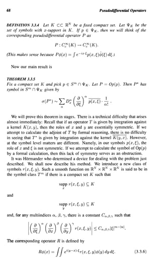
Let r E T m have x- and y-supports contained in a compact set K. Then
the operator R defined as in (3.3.6) defines a pseudodifferential operator of
Kohn-Nirenberg type with symbol pEW K having an asymptotic expansion
p(x,~) '" L ~!alD~r(x,~,y)ly=x'
n
PROOF We calculate that
JeiY'~r(x, ~,y )¢>(y) dy = (r(x, ~, .)¢>(-))
= (i3 (x, y, .) * J(-)) (~).
Here f3 indicates that we have taken the Fourier transform of r in the third
variable. By the definition of R¢ we have
R¢>(x) = JJei(-x+Y)'~r(x,~,y)¢>(y)dyd~
J
= e-ix.~ [i3(x,~,.) * J(-)] (~) d~
= JJi3(x,~, ~ - TJ)J(TJ) dTJe-ix,~ d~
= JJi3(x,~, ~ - TJ)e-ix,(~-'f}) d~J(TJ)e-ix.'f} dT]
== J p(x, y)J(TJ)e-ix.'f} dTJ·
Here
Ji3(x,~, ~ TJ)e-ix(~-'f}) ~
p(x, TJ) == -
=Je-ix'~i3(x, ~ + TJ,~) d~.
Now if we expand the function f3 (x, TJ + .,~) in a Taylor expansion in powers
of ~, it is immediate that p has the claimed asymptotic expansion. In particular,
one sees that p E sm. In detail, we have
i3(x, 1] +~,~) = L a;i3(x, TJ,~) ~~ + R.
Inl<k](https://image.slidesharecdn.com/partialdifferentialequationsandcomplexanalysis-121120212851-phpapp02/85/Partial-differential-equations-and-complex-analysis-80-320.jpg)
![70 Pseudodifferential Operators
Thus (dropping the ubiquitous c from the Fourier integrals),
p(x,Tj) = L 1e-iX'€8;f3(x,Tj,~):~ d~ + 1Rd~
lal<k
= L ~!8;D~r(X,Tj,y)ly=x + 1 Rd~.
lal<k
The rest is formal checking. I
PROOF OF THEOREM 3.3.5 Let pEW K n sm
and choose cP, 1/J E V. Then,
with P the pseudodifferential operator corresponding to the symbol p, we have
(dJ, P* 1/J) == (PcP, 1/J)
= 1[1 e-iX'€p(X,~)¢(~)d~] "j;(x)dx
= 1 1e-i(x-YH4>(y)dyp(x,~)d~"j;(x)dx.
1
Let us suppose for the moment that p is compactly supported in~. With this
extra hypothesis the integral is absolutely convergent and we may write
(4), P*7/J) = 14>(Y) [11 ei(x-y)·€ p(x, ~)7/J(x) d~ dx ] dy. (3.3.5.1)
Thus we have
P*7/J(y) = 1 ei(x-YHp(x,~)7/J(x)d~dx.
1
Now let p E C~ be a real-valued function such that p == 1 on K. Set
r(x,~,y) == p(x)· p(y,~).
Then
P*7/J(y) =11 ~)p(Y)7/J(x) d~
ei(x-YH p(x, dx
=1ei(x-YHr(y,~,x)7/J(x)d~dx
== R1/J(y),
where we define R by means of the multiple symbol r. (Note that the roles of
x and y here have unfortunately been reversed.)](https://image.slidesharecdn.com/partialdifferentialequationsandcomplexanalysis-121120212851-phpapp02/85/Partial-differential-equations-and-complex-analysis-81-320.jpg)
![The Calculus of Pseudodifferential Operators 71
By Proposition 3.3.7, P* is then a classical pseudodifferential operator with
symbol p* whose asymptotic expansion is
p*(x,~) '" ~ ~! of D; [p(x)p(y, ~)] Iy=x
'" L J,af D';p(x, ~).
Q.
a
We have used here the fact that p == 1 on K. The theorem is thus proved with
the extra hypothesis of compact support of the symbol in ~.
To remove the extra hypothesis, let ¢ E ergo satisfy ¢ == 1 if I~ I ~ 1 and
¢ == 0 if I~I 2: 2. Let
Observe that Pj ~ P in the e k topology on compact sets for any k. Also, by
the special case of the theorem already proved,
The proof is completed now by letting j ~ 00. I
THEOREM 3.3.8 KOHN-NIRENBERG
Let P E l1 K n sm, q E l1 K n sn. Let P, Q denote the pseudodifferential
operators associated with p, q respectively. Then Po Q == Op(a) where
1. a E l1 K n sm+n;
2. a ~ La ~8rp(x, ~)D~q(x, ~).
PROOF We may shorten the proof by using the following trick: write Q =
(Q*) * and recall that Q* is defined by
Q*¢J(y) = / / ei(x-YH¢J(x)q(x,~)dxd(,
= (/ eix'~¢J(x)q(x,~) dx ) ---- (y).
Here we have used (3.3.5.1).
Then
Q¢J(x) = (J eiY·~¢J(y)q.(y,~) dy) ---- (x), (3.3.8.1 )](https://image.slidesharecdn.com/partialdifferentialequationsandcomplexanalysis-121120212851-phpapp02/85/Partial-differential-equations-and-complex-analysis-82-320.jpg)
![72 Pseudodifferential Operators
where q* is the symbol of Q*. (Note that q* is not if; however, we do know
that if is the principal part of q*.) Then, using (3.3.8.1), we may calculate that
(P 0 Q)(¢»(x) = J e-ix·ep(x, ~)(Q¢)(O d~
= JJe-ix·ep(x,Oeiy·eq*(y,~)¢>(y)dyd~
= JJe-i(x-y)·e [p(x,~)q*(y,~)] ¢>(y)dyd~.
Set q == q*. Define
r(x,~, y) == p(x,~) . ij(y, ~).
One verifies directly that r E Tn+m. We leave this as an exercise. Thus R,
the associated operator, equals P 0 Q. By Proposition 3.3.7 there is a classical
symbol a such that R == Op( a) and
a(x,O "-J L ~! of D~r(x,~, y)ly=x'
Q
Developing this last line we obtain
a(x,O "-J L ~!OfD~ (p(x,Oq(y,~))ly=x
Q
"-J L ~!Of [p(x,OD~q(y,O] Iy=x
Q
"-J L ~or [p(x,OD~q(x,O]
o.
Q
"-J L all! [or1p(x,o] a;! [otD~2D~lq(X,~)]
QI,Q2
QI
'""" oI! 8 ~ p ( x, ~ ) D x
~ 1 ~ 0 1 ! 8Q2 D x q x, ~ ) ]
2 ~
QI ['""" Q2 _(
f"V
QI Q2
"-J L ~o{p(X,~)D~lq(X,~).
0'.
QI](https://image.slidesharecdn.com/partialdifferentialequationsandcomplexanalysis-121120212851-phpapp02/85/Partial-differential-equations-and-complex-analysis-83-320.jpg)
![The Calculus of Pseudodifferential Operators 73
Here we have used the fact that the expression inside the brackets is just the
asymptotic expansion for the symbol of (Q*) *. That completes the proof. I
The next proposition is a useful device for building pseudodifferential oper-
ators. Before we can state it we need a piece of terminology: we say that two
pseudodifferential operators P and Q are equal up to a smoothing operator if
P - Q E Sk for all k < O. In this circumstance we write P rv Q.
PROPOSITION 3.3.9
Let Pj, j == 0, 1,2, ..., be symbols of order mj, mj ~ -00. Then there is a
symbol P E smo, unique modulo smoothing operators, such that
PROOF Let 'l/J : ~n ~ [0, 1] be a Coo function such that 'l/J == 0 when Ixl ::; 1
and 'l/J == 1 when Ixl 2: 2. Let 1 < t l < t2 < ... be a sequence of positive
numbers that increases to infinity. We will specify these numbers later. Define
00
p(x,~) == L 'l/J(~/tj )Pj (x, ~).
j=O
Note that for every fixed x, ~ the sum is finite, for 'l/J (~/ tj) == 0 as soon as
tj> I~I. Thus P is a well-defined Coo function.
Our goal is to choose the tj'S so that P has the correct asymptotic expansion.
We claim that there exist {t j} such that
Assume the claim for the moment. Then for any multiindices Q, {3 we have
00
ID~Drp(x,~)1 ::; L ID~Dr ('l/J(~/tj)Pj(x,~))1
j=O
00
::; L2- (1 + 1~l)mJ-IQI
j
j=O](https://image.slidesharecdn.com/partialdifferentialequationsandcomplexanalysis-121120212851-phpapp02/85/Partial-differential-equations-and-complex-analysis-84-320.jpg)
![74 Pseudodifferential Operators
It follows that p E sm
o• Now we want to show that p has the right asymptotic
°
expansion. Let < k E Z be fixed. We will show that
k-l
p- LPj
j=O
lives in smk. We have
k-l
- L (l-7/J(~/tj))Pj(x,~)
j=O
== q(x,~) + s(x, ~).
It follows directly from our construction that q(x,~) E k
sm
• Since [l-'ljJ(~/tj)]
has compact support in B(O, 2t l ) for every j, it follows that s(x,~) E S-oo.
Then
k-l
P - LPj E sm k
j=O
as we asserted.
We wish to see that P is unique modulo smoothing terms. Suppose that
qE smo and q L~OPj. Then
f"V
P- q== (p - LPj) - (q - LPj)
J<k J<k
for any k. That establishes the uniqueness.
It remains to prove the claim. First observe that, for lad == j,
IDf7/J(~/tQ)1 = ik I(Df7/J) (~/tj)1
t·
J
+
~ tjl I1€1::;2t
sup
J
{(DQ'lj;). (1 + I~I)IQI}I (1 + I~I)-IQI](https://image.slidesharecdn.com/partialdifferentialequationsandcomplexanalysis-121120212851-phpapp02/85/Partial-differential-equations-and-complex-analysis-85-320.jpg)
![4
Elliptic Operators
4.1 Some Fundamental Properties of Partial Differential Operators
We begin this chapter by discussing some general properties that it is desirable
for a partial differential operator to have. We will consider why these proper-
ties are desirable and illustrate with examples. We follow this discussion by
introducing an important, and easily recognizable, class of partial differential
operators that enjoy these desirable properties: the elliptic operators.
Our first topic of discussion is locality and pseudolocality. Let T : C~ ~
Coo. We say that T is local if whenever a testing function ¢ vanishes on an
open set U then T¢ also vanishes on U. The most important examples of local
operators are differential operators. In fact, the converse is true as well:
THEOREM 4.1.1 PEETRE
If
T: Cr: ~ COO
is a linear operator that is local then T is a R.artial differential operator.
PROOF See [HEL]. I
The calculation of a derivative at a point involves only the values of the
function at points nearby. Thus the notion of locality is well suited to differ-
entiation. In particular, it means that if T is local and ¢ == 'l/J on an open set
then T¢ == T'l/J on that open set. For the purposes of studying regularity for
differential operators, literal equality is too restrictive and not actually necessary.
Therefore we make the following definitions:
DEFINITION 4.1.2 Let ex E V' and U ~ IR N an open set. If there is a Coo](https://image.slidesharecdn.com/partialdifferentialequationsandcomplexanalysis-121120212851-phpapp02/85/Partial-differential-equations-and-complex-analysis-87-320.jpg)
![Properties of Differential Operators 77
function f on U such that for all ¢ E V that are supported in U we have
n(¢» = 1 j(x)¢>(x) dx,
then we say that 0 is Coo on u.
The singular support of a distribution 0 is defined to be the complement of
the union of all the open sets on which 0 is Coo.
DEFINITION 4.1.3 A linear operator T : V' ~ V'is said to be pseudolocal
if whenever U is an open set and 0 E V'is Coo on U then To is Coo on U.
Now we have
THEOREM 4.1.4
If T is a pseudodifferential operator, then T is pseudoloeal.
The theorem may be restated as "the singular support of Tu is contained in the
singular support of u for every distribution u."
A sort of converse to this theorem was proved by R. Beals in [BEA2-4]. That
is, in some sense the only pseudolocal operators are pseudodifferential. We shall
not treat that result in detail here.
The proof of the theorem will proceed in stages. First, we need to define how
a pseudodifferential operator operates on a distribution. Let P be a pseudodif-
ferential operator and let u E V' have compact support. We want Pu to be a
distribution. For any testing function ¢, we set
(Pu, ¢) == (u, t P¢).
Here t P is the transpose of P which we define by
for ¢,'l/J E V.
To illustrate the definition, suppose that u is given by integration against an
Ll function f. Suppose also that the pseudodifferential operator P is given by
integration against the kernel K(x, x - y) with K(·, y) E L 1 and K(x, .) ELI.
Then P has symbol K (x, ~). We see that
2
(Pu)(¢» = 1[1 K(x,x-y)j(Y)dY] ¢>(x)dx
=J~ K(x, x - y)¢>(x) dX] j(y) dy
=J t P¢>(y)f(y) dy.](https://image.slidesharecdn.com/partialdifferentialequationsandcomplexanalysis-121120212851-phpapp02/85/Partial-differential-equations-and-complex-analysis-88-320.jpg)
![82 Elliptic Operators
for x E suppp(·,~), ~ large with a(x) > 0 a continuous function. Select a
relatively compact open set L ~ supp p(.,~) so that there is a constant CO > 0
with a(x) > Co on L. We also select Ko > 0 such that, for I~I 2: K o and x E L,
it holds that Ip(x,~)1 2: col~lm. Let'l/J be a C~ function with support in the
(x variable) domain of a(P) such that 'l/J == 1 on L. Also choose a function
¢ E Coo such that ¢(~) == 1 for I~I 2: K o + 2 and ¢(~) == 0 for I~I :::; K o + 1.
Then set
and
Qo == Op( qo).
Observe that ¢ == 0 on a neighborhood of the zeroes of p(x, ~); hence qo is Coo.
Furthermore, qo has compact support in x. Finally, qo E s-m. To see this, first
notice that
Moreover,
la~j qo(X,~)1 = '1/J(X)'·lp(x,~)(ac/>/a~j)~l(:,~~~)(ap(x,o/a~j) I
< C. [(1 + IW ·1(a¢>/a~j)(~)1 + (1 + IW
m m 1
- ]
- (1 + 1~1)2m (1 + 1~1)2m
for lei large. But this is
However, B¢/ Bej is compactly supported, so it follows that
Arguing in a similar fashion, one can show that
Since x derivatives are harmless, we conclude that qo E s-m.](https://image.slidesharecdn.com/partialdifferentialequationsandcomplexanalysis-121120212851-phpapp02/85/Partial-differential-equations-and-complex-analysis-93-320.jpg)
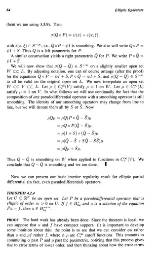
![Regularity for Elliptic Operators 85
would affect the parametrix.) Let 'l/J E C~ satisfy'l/J == 1 on suppu. Let Q be
a left parametrix for P:
S == QoP - 'l/JI
is smoothing. Then
u == 'l/Ju == (Q 0 P - S)u == Qf - Suo
Since f E H S and Q is of order -m, it follows that Qf E H s +m ; also, Su is
smooth. Then Qf - Su E Hs+m, that is, u E Hs+m. I
Now that we have our basic regularity result in place we will use it, and some
functional analysis, to prove our basic existence result. We would be remiss
not to begin by mentioning the paramount discovery of Hans Lewy in 1956
[LEW2]: not all partial differential operators are locally solvable. In fact, we
shall discuss Lewy's example in detail in Chapter 9.
Although we do not attempt to fonnulate the most general local solvability
result, we present a result that will suffice in our applications. The most impor-
tant ideas connected with local solvability of partial differential operators appear
in [NTR], [BEFI], and the references therein.
THEOREM 4.2.5
Let P be an elliptic partial differential operator on a domain o. If f E V'(O)
and Xo E 0, then there exists a u E D' (0) such that Pu == f in a neighborhood
ofxo.
PROOF We may assume, by the usual arguments, that f has compact support-
that is, f E ['. Then f E H S for some s. Thus we may take the partial
differential operator P to have compact support in a neighborhood K of Xo.
Let 'l/J E C~ (0) satisfy 'l/J == 1 on K. Let Q be a right parametrix for P such
that
Po Q - 'l/JI == S (4.2.5.1)
and S is smoothing. By looking at the left side of this equation we see that
a(S) has x-support also lying in supp'l/J. Thus
S: H S ~ C~(supp'l/J).
Then S : HS ~ HS is compact by Rellich's lemma. Therefore the equation
(S + I)u == f (4.2.5.2)](https://image.slidesharecdn.com/partialdifferentialequationsandcomplexanalysis-121120212851-phpapp02/85/Partial-differential-equations-and-complex-analysis-96-320.jpg)
![00 Elliptic Operators
can be solved if fEN 1-, where
N == {g E H
S
: (S* + 1)g == O};
here the inner product is with respect to the Hilbert space HS. Notice that, since
S* is also smoothing (why?) and 9 == -S* 9 for 9 E N, we know that N is a
finite-dimensional space of Coo functions.
Let gl , ... , 9 M be a basis of N. We claim that there exists a neighborhood U
of Xo such that gl , ... , 9 M are linearly independent as functionals on C~ (0 U).
To see this, suppose that U does not exist. Let Un be neighborhoods of Xo such
that Un '. xo. For each n, let C l, ... ,CnM be constants (not all zero) such that
n
M
G n == LCnjgj == 0
j=1
as functionals on C~(O Un). By linearity, we may suppose that each G n has
nonn 1 in N for all n (note in passing that G n -# 0 for every n). Since N is finite
dimensional, there is a convergent subsequence G nm such that G nm ~ G E N
and G has nonn 1. However, viewed as a functional on C~(O), G has support
{xo}. Since G is Coo, we have a contradiction.
Thus we have proved the existence of U. We may assume that U cc K.
Now we can find a Coo function h with support in 0 U such that f + h is
perpendicular to N in the HS(O) topology. By (4.2.5.2), there is a distribution
u such that
(1 + S)u == h + f == f on U.
By (4.2.5.1), we see that P (Qu) == f on U. Therefore Qu solves the differential
equation. I
Exercise: The proofs of the last two theorems, suitably adapted, show that
the local solution exhibits a gain in smoothness, in the Sobolev topology, of
order m.
It is also the case that elliptic partial differential equations exhibit a gain of
order m in the Lipschitz topology. We shall present no details for this assertion.
Given the machinery that we have developed, it is only necessary to check that
if p Esm then Op(p) : A~c ~ A~~m for any Q > O. This material is discussed
in [TAY].
Exercise: Prove that the elliptic operator P in Theorem 4.2.5 is surjective in a
suitable sense by showing that its adjoint is injective.](https://image.slidesharecdn.com/partialdifferentialequationsandcomplexanalysis-121120212851-phpapp02/85/Partial-differential-equations-and-complex-analysis-97-320.jpg)
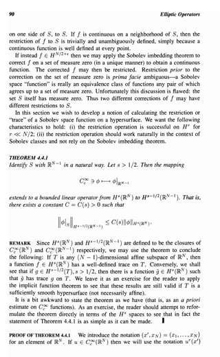
![Restriction Theorems for Sobolev Spaces 91
to denote u(x', 0). Now we have
Ilu r l/;JS-l/2(IRN - = { 11?(e)ll + WI 2)S-I/2 de
J~N-l
1)
== r [_ J(')O ~IUi(e,xN)12(1
J~N-l o aXN
+ leI 2)S-I/2 dXN] d~'.
Here UI denotes the partial Fourier transform in the variable x'. The product
rule yields that, if D is a first derivative, then D(lhI 2) ::; 2Ihl·IDhl. Therefore
the last line does not exceed
2 {
J~N-l Jo
to IUi(e,XN)I.la XN Ui(e,XN)I. (1 + 1~'12)s-I/2dxNd~'.
8
Since 20:(3 ::; 0: 2 + (32, the last line is
2
: :; J~N-l JtOla8 Ui (e,XN)1
( o XN dXN(1+WI 2)S-lde'
== I + II.
Now apply Plancherel's theorem to term I I in the x N variable. The result is
II :::; C IN-1 llu(e,eN)1 2 deN(l + lel 2
)" de
::; Cllull~s(~N).
Plancherel '8 theorem applied, in the x N variable, to the term I yields
2
I::;C r J~ laXN Ui(e,XN)1
J~N-l
r 8 dXN(1+leI 2)S-Id1,'
: :; err IU(e,~N)12 ·1~NI2d~N(1 + leI 2)S-Id1,'
J~N-l JJR
:::; C { lu(~)12. (1 + 1~12)sd1,
J~N
I
As an immediate corollary we have:
COROLLARY 4.4.2
Let u E HS(lR N ) and let 0: be a mu!tiindex such that s > lal + 1/2. Then nau
has trace in Hs-la l-I/2(lRN - 1 ).](https://image.slidesharecdn.com/partialdifferentialequationsandcomplexanalysis-121120212851-phpapp02/85/Partial-differential-equations-and-complex-analysis-102-320.jpg)
![92 Elliptic Operators
Now we present a converse to the theorem. Again set S == {(x', 0) E IR N }.
THEOREM 4.4.3
Assume that cPo, ... , cPk are defined on S, each cPj E Hs-j-l/2CIR N - 1 ) with
s > 1/2 + k. Then there exists a function f E HS (IR N ) such that D~ f has
trace cPj on S, j == 0, ... ,k. Moreover,
k
IIfIlHs(~N) ~ Cs,k L IlcPjllks-J-I/2(~N-I).
j=O
PROOF Let h E C~ (IR), h == 1 in a neighborhood of the origin, 0 ~ h ~ 1.
We define
and
This is the function f that we seek. For if m is any integer, 0 ~ m ~ k, then
==
J. e -'LX
I
.~ I 'm ~ _1
l
k
~.,
j=O J.
(m)
.
J
"
.
J. ( _ l')J
x 8:-~j [h(xN(l + 1e1 2)1/2)] I . ¢;(~') d~'
8x N XN=O
= J e- ix ',( ¢;;,(e) de
== cPm(X').
This verifies our first assertion.](https://image.slidesharecdn.com/partialdifferentialequationsandcomplexanalysis-121120212851-phpapp02/85/Partial-differential-equations-and-complex-analysis-103-320.jpg)
![94 Elliptic Operators
Then (4.4.3.1) is
k
::; Cf; (j~)2 kN-l k Ih(j)(~N)12 (1 + 1;'1 2)1+ 1(1 + leI 2)1/2
xl¢;(~/) 1 [( 1 + 1 ) (1 + 1N 1) ] s d~' d~ N
2
~/12 ~ 2
k
= CL: ~ (
(J.)
j=O JRN-I
l¢j(OI2(1 + leI 2)S-j-I/2de
X kIh(j)(~N )1 (1 + I~NI2)s d~N
2
k
~ Cs,k L: lI¢jll~s-j-I/2(~N-I).
j=o
That completes the proof of our trace theorem. I
REMARK The extension iii was constructed by a scheme based on ideas that
go back at least to A. P. Calderon-see [STSI] and references therein. I](https://image.slidesharecdn.com/partialdifferentialequationsandcomplexanalysis-121120212851-phpapp02/85/Partial-differential-equations-and-complex-analysis-105-320.jpg)
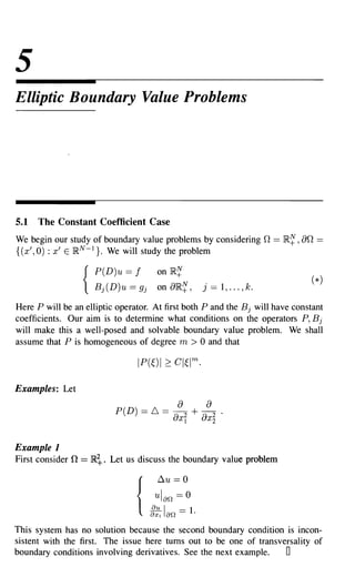
![The Constant Coefficient Case 97
For each fixed ~' == (~1, ... ,~N -1), we consider P(~', D N). We will solve
as an ordinary differential equation. Thus our problem has the fonn
m
Lap(t)
( d
dx
)£ v = o.
£=0 N
The solution ,v of such an equation will have the form
r(~/) VJ-I
V(XN) == L L Cj£(~')(XN )£eiXN~j(~/),
j=1 £=0
where Al (~'), A2 (~'), ... , Ar (~') are the roots of P (~', . ) == 0 with multiplicities
VI (~'), V2(~'),' .. ,Vr(~').
We restrict attention to those Aj with positive real part. Since these roots
alone will be enough to enable us to carry out our program, this choice is
justified in the end. However, an a priori theoretical justification for restricting
attention to these A'S may be found in [HOR1].
After renumbering, let us say that we have retained the roots
Al (~' ), ... , Aro ( ~') , TO :::; T.
Then
ro v J - l
V == L L Cj£(~')(XN )£eiXN~j(~/).
j=1 £=0
Fact: A fundamental observation for us will be that the number TO of roots
(counting multiplicities) with positive imaginary part is independent of ~' E
]RN -1 {O}. This is proved by way of the following two observations:
(i) Each Aj (~'), j == 1, ... , TO, depends continuously on ~'.
(ii) There are no Aj with zero imaginary part (except possibly A == 0).
We leave it to the reader to supply the details verifying that these two obser-
vations imply that the number of roots is independent of ~' (use the ellipticity
for (ii». Now we summarize the situation: our problem is to solve, for fixed
~', the system
P(~/, DN)v == 0 on 1R~
Bj(~', DN)v == gj(€') on 8IR~ ,j = 1, ... , k. (5.1.1)
From now on we take k to equal Vo + ... + V ro '](https://image.slidesharecdn.com/partialdifferentialequationsandcomplexanalysis-121120212851-phpapp02/85/Partial-differential-equations-and-complex-analysis-108-320.jpg)
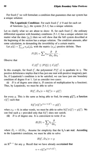
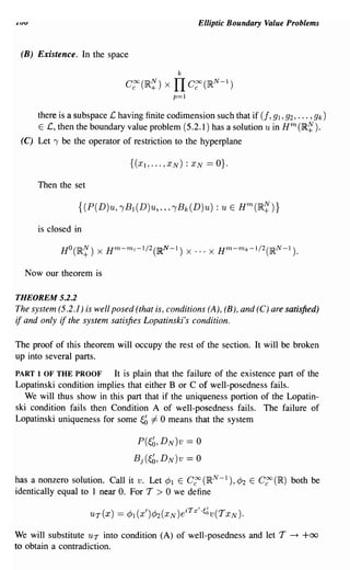
![Well-Posedness 101
First observe that lIuT I sup < 00. Now let Q
multiindex of order m. We calculate that
IIUTIIHm 2: IIDQuTII~o
=JID~, [¢JI(X')¢J2(xN)eiT(X"~~)v(TXN)] 1
2
dx'dxN
~ JI¢JI(x')¢J2(xN)(~~)aTla'V(TxN)12
C dx'dxN
2
- c J L C/3ID~,[¢JI(X')]¢J2(XN)(~~)'Thlv(TxN) dx'dxN
13+,=0
1131>0
2
-~ J L 13+,=0
C/3ID~,[¢JI(X')]¢J2(XN/T)(~~)'Thlv(XN) dx'dxN
1/31>0
2: cT T- 2m 1 - C'T 2m - 2T- 1
2: cr2m - 1
for T large. Therefore
(5.2.2.1)
for T large. On the other hand,
P(D)UT = P(D) [¢JI(X')¢J2(xN)eiTX"~~v(TxN)]
= ¢JI (X')¢J2 (x N)P(D) [e iTX ' '~~v(T xN)]
+ (terms in which a derivative falls on a cutoff function)
== 0 + (terms in which fewer than m derivatives
fall on eiTxl'~~v(TxN))' (5.2.2.2)
We have used here the fact that
P(D) [eiT(X"~~)v(TxN)] = P(T~~, TDN)vI TxN
== T m P(~b, D N )vl TxN
== o.](https://image.slidesharecdn.com/partialdifferentialequationsandcomplexanalysis-121120212851-phpapp02/85/Partial-differential-equations-and-complex-analysis-112-320.jpg)
![102 Elliptic Boundary Value Problems
As a result, from (5.2.2.2), we obtain
IIP(D)uTII~ ::; CT2m - 2
. (5.2.2.3)
Similarly,
Bj(D) [eiTX"~~v(TxN)] = Bj(T~~, TD N )vl TxN
== TmJ Bj(~b, D N )vI TxN ·
Therefore
Bj(D)[uyJ = Bj(D) [¢>I(X')¢>2(xN)eiYX"~~v(TxN)]
== 0 + terms in which derivatives of total order
not exceeding mj - 1 land on eiTxl·~~v(TxN).
As above,
2m 3
I J m-m J -1/2 < C [TmJ-1+m-mJ-1/2]2 == CT - •
I B·(D)u T 112 - (5.2.2.4)
Therefore, substituting UT into condition (A) of the definition of well-posedness,
we obtain (from (5.2.2.1), (5.2.2.3), and (5.2.2.4» that
CT 2m - 1 ::; C'T 2m - 2 + C".
This inequality leads to a contradiction if we let T ---+ +00.
PART 2 OF THE PROOF Assume that the Lopatinski condition holds at all
~' =1=O. We will prove that the system is well posed. This argument will
proceed in several stages and will take the remainder of the section.
Let u E Hm (IR~) be a solution of
P(D)u == 0 on IR~
{ Bj(D)u == 0 on aIR~, j == 1, ... , k.
Let
Then
P(~',DN)V==O onn
{ Bj(~',DN)V == 0 on an.
The general solution of P(~', D N)V == 0 looks like
ro v J -1
V(~',XN) == L L Cj£(~')(XN)£eiXN~j(().
j=1 £=0
But the Lopatinski hypothesis then guarantees that such a v == 0 so that u == O.](https://image.slidesharecdn.com/partialdifferentialequationsandcomplexanalysis-121120212851-phpapp02/85/Partial-differential-equations-and-complex-analysis-113-320.jpg)

![106 Elliptic Boundary Value Problems
Here, of course, we have used the standard restriction theorem for Sobolev
spaces.
Now this last line is
because £ is an operator of order -me We apply the partial Fourier transform,
denoted by -, in the x' variable to transform our system to
P(~', DN)v == 0 on }RN
+
Bj(~', DN)v == hj on a}R~, j == 1, ... , k. (5.2.4.1)
By Lopatinksi's condition, the space of solutions of the first equation that de-
crease exponentially has finite dimension (indeed k dimensions) and the map
is one-to-one and onto. Thus a solution to (5.2.4.1) exists. By the fact that all
norms on a finite-dimensional vector space are comparable (alternatively, by the
open mapping principle),
f1
j=O 0
00
ID{yv((,XNWdxN + Y:
j=O
ID{yv((,O)1 2 :::; C2(() t Ih (012.
j=1
j
Here the right-hand side represents a norm on the space of k-tuples, while the
left-hand side is a norm on the solution space of the boundary value problem.
Now by direct estimation, or using Theorem 10.2.1 of [HOR1], we obtain
L: Ihj (()1 2 :::; C· (L: 19j((W + L: IB ((,DN)U((,O)1 2) j
) ) )
[~19j(012 + 1 11((, XN )1 2dXN] .
00
:::; C3 (0
The constant C (~') is a continuous function of ~' (since it arises from the
inversion of a matrix with continuous coefficients). Therefore it is bounded
above and below on {~' : I~'I == I}. We conclude that
f1
)=0 0
00
IDi¥v((,XN)2dxN + Y:
j=O
ID{yv((,OW
[~l§j(()12 + 1 11((, XN )1 2dXN]
00
:::; Co](https://image.slidesharecdn.com/partialdifferentialequationsandcomplexanalysis-121120212851-phpapp02/85/Partial-differential-equations-and-complex-analysis-117-320.jpg)
![Well-Posedness 107
provided that I~' I == 1. Let r > 0 be a constant. Then any inequality that holds
for the original system
P(D)u == f
Bj(D)u == gj, j == 1, ... , k
must also hold for the system
P(rD)u == r m f
Bj(rD)u == rmJgj, j == 1, ... ,k
when I~' I == 1I r. Putting this information into our inequality, and substituting
I~'I for 1/r, yields that
J
Adding Iv(~', XN )1 2 dXN to both sides of the inequality and integrating in the
~' variable yields
IlvllkTn(~N) + Ilv(x', 0) IlkTn-I/2(~N-I)
:::; Co [llfll~O(IRNl + 1; Ilgjll~m-mj-1/2(IRN-ll + IIVIIHO(IRNl] .
This is just the sort of estimate that we seek for the finite dimensional solution
space of the system
P(D)v == 0
Bj(D)v == h j .
Combining this with the obvious estimate
gives the estimate that we need for part (A) of well-posedness. Our proof is
therefore complete. I](https://image.slidesharecdn.com/partialdifferentialequationsandcomplexanalysis-121120212851-phpapp02/85/Partial-differential-equations-and-complex-analysis-118-320.jpg)
![108 Elliptic Boundary Value Problems
5.3 Remarks on the Solution of the Boundary Value Problem in the
Constant Coefficient Case
We have considered the boundary value problem
P(u) == f
B.V.P. { B j U == 9 j if j == l, ... , k.
Here the operator P is assumed to have constant coefficients, to be elliptic, and
to be homogeneous of degree m. We assume that the Bj's satisfy the Lopatinski
nondegeneracy condition.
For ~' fixed, we examined
if XN >0
if XN == 0, j == l, ... ,k.
Lopatinski's condition tells us that this is a well-posed linear system of ordinary
differential equations. Thus the standard classical theory of ordinary differential
equations (see [HORl], [INCE], or [COL]) guarantees that there is a unique
solution Ul (~/, XN).
The solution that we seek for the B.V.P is
For if is the partial Fourier transform, then
Properties of this solution u are
1. u is unique.
2. The map (f, 91, ... , 9k) ~ u is linear.
3. Define
k
1t == L2(IR~) x IT H m- m j-l/2(lRN - 1 ).
j=1
There are two basic ingredients to seeing why property (3) holds:
(i) Solving an ordinary differential equation in the x N variable entails m
integrations, so u should be m degrees smoother in the x N direction
than f.](https://image.slidesharecdn.com/partialdifferentialequationsandcomplexanalysis-121120212851-phpapp02/85/Partial-differential-equations-and-complex-analysis-119-320.jpg)
![110 Elliptic Boundary Value Problems
where F == (f, 91, ... ,9k). Here 1t is the usual product Hilbert space and the
operator
is defined by
Au == (Pu, ,B1u, ... , ,Bku).
The error operators T, T 1 are compact operators on Hm (1R~) and 1-l, respec-
tively. The operator, denotes restriction.
Main Results
THEOREM 5.4.1
Assume that our boundary value problem satisfies the Lopatinski condition as
defined above. Assume that f E L2(~~), 9j E Hm-mJ -1/2(~N -1). Then there
is a linear operator
E: 1t ~ Hm(~~)
such that if F == (f, 91, ... , 9k) and u == E(F), then
Au == F + TF,
where T is of order -1 and
PROOF We assume for convenience that the coefficients of P and of the Bj's
have compact support. We will make decisive use of the hypothesis that the
coefficients are smooth. [Much modem research concentrates in part on studying
elliptic and other problems with rough coefficients. From the point of view of
applications, such a study is rather natural (see [MOS] for some of the pioneering
work and [FKP] for more recent work along these lines). But the necessary
techniques are extremely complicated and we cannot explore them here.]
Now let E > O. Then there is a 8 > 0 such that if Ix - yl < 8 and if a is any
coefficient of P or of one of the Bj's then
la(x) - a(y)1 < Eo
Let <Pj E ergo (~N), cPj 2 0, L cPj == 1 on ~N. Assume that diam supp cPj <
8/2. We can assume that no point x is in more than M (N) of the supports of
the <pj's. (If we take the supports to be balls, then in fact we may take M (N)
to be N + 1.) Now choose functions 1/Jj E ergo (~N) such that 1/J == 1 on the
support of cPj. We may also assume that diam supp 1/Jj < 8/2. (The trick of
choosing cutoff functions 1/J that are identically equal to 1 on the support of](https://image.slidesharecdn.com/partialdifferentialequationsandcomplexanalysis-121120212851-phpapp02/85/Partial-differential-equations-and-complex-analysis-121-320.jpg)
![Solution of the Boundary Value Problem in the Varitlble Coefficient Case 111
some smaller cutoff functions ¢ is a device of wide utility in this subject. We
already saw it enter into our study of interior estimates for elliptic operators. We
will see it put to particularly good use when we study the 8- Neumann problem
in a later chapter.)
Define Wj to be the support of 1Pj. If, for some £, Wi n aIR~ == 0, then
we choose a point xl E Wl and construct a parametrix Ei for the constant
coefficient problem
where Pm is the principal symbol of P. Next we treat the other £' s.
If Wl n aIR~ :/: 0 then select xl E Wl n aIR~. By our work on the boundary
value problem for the constant coefficient case, we may find for each £ an
operator
such that the function
satisfies
and
Now we set
Define an approximate solution of our boundary value problem by u = Eo(F),
where F == (f, gl, ... ,gk). Then
P(x, D)Eo(F) == L P(x, D) [¢lEl 1Pl F ]
l
== L ¢lP(X, D) (El1PlF)
l
+ L (
some )
derivative
( At most
(m - 1) derivatives
)
e of ¢e of Ef'l/Je F](https://image.slidesharecdn.com/partialdifferentialequationsandcomplexanalysis-121120212851-phpapp02/85/Partial-differential-equations-and-complex-analysis-122-320.jpg)
![112 Elliptic Boundary Value Problems
== L ¢£P(x, D) (E£1};£F) + OP m - I (E£1};£F)
£
== L ¢£Pm(x£, D) (E£1};£F)
£
+ L ¢£ [Pm(x, D) - Pm(x l , D)] (EL'l/JlF)
£
+ L [P(x, D) - Pm(x, D)] (El'l/JlF)
£
+ OPm - I (E£1};£F)
== I + II + III +OPm-I(El'l/JlF).
By the definition of E£, we have
I == L ¢£1P£f + lower order errors
£
where 5 I f E HI when f E HO. Set II == TF and III == TIF, where T is the
sum of operators from H into HO with arbitrarily small norms (depending on E)
and T I is an operator mapping H to HI. (Observe that the assertion about the
size of the norm of T follows immediately from the presence of the coefficients
[Pm(x, D) - Pm(x£, D)], which are uniformly small.)
In summary, we have
Similarly, we can calculate B j (x, D)EoF and obtain that
Bj(x, D)EoF == L [¢£1P£gj] + TjF + TJ F + SJF.
£
Here T j and T) are operators with properties analogous to those of T and T 1•
Let
Then we can summarize our findings with the equation
AEoF == F + UF + UIF, (5.4.1.1)](https://image.slidesharecdn.com/partialdifferentialequationsandcomplexanalysis-121120212851-phpapp02/85/Partial-differential-equations-and-complex-analysis-123-320.jpg)
![114 Elliptic Boundary Value Problems
We would like now to show that if
then
The experience that we have so far with pseudodifferential operators suggests
that they will serve us well in this endeavor.
We begin by defining As to be the pseudodifferential operator with symbol
(1 + 1~/12) oS /2. (In other contexts this operator is known as a tangential Bessel
potential of order s. See [STSI] and [FOK].) We will use these extensively in
Chapter 7. Let F E KS. Then AsF E H and hence EAsF E Hm. But As
commutes with A (up to a lower order error) so that EA s == AsE + (error) and
we find that E == A; 1EA s modulo a smoothing error term. In conclusion, if
u == EF then Asu E Hm.
With these preliminaries out of the way, we begin by treating the case 0 <
s ~ 1. Write P(x, D) == DlJ + Do, where Do involves terms of the fonn
Dr;;-jDf,lod ~ j, and 0 < j ~ m. To see that Dr;;-jDfu E HS, it suffices
for us to check that
But
1i5fU1 (1 + 1~12)(m-j+s)/2 :S lilll(l j
(1 + 1~12)(m-j+s)/2
== 1~/lsl~/lj-S(l + 1~12)(m-j+s)/2Iul
~ 1~/ISlul(l + 1~12)m/2.
We have used here the fact that 0 < s ~ 1 ::; j. The latter expression is clearly
in £2 since Asu E Hm. Finally, since Pu == f, we have that DlJu E HS (from
the partial differential equation itselt). Hence u E H m + s .
Next, if 1 < s ~ 2, then As-1u E Hm+l and with the same argument as
above we may see that u E Hm+s. The result for higher s follows inductively
by similar arguments.
In summary, we have proved that
Ilull s+m ~ C (II Au lls + Ilulls)
=c (IIPUIIHS(IR~) + "t.IIBjUlls+m-mJ-1/2 + IIUlls) .
Now we vindicate the form that our program has taken (that is, concentrating
on regularity estimates in the absence of existence results) by using our regularity
theorems together with some functional analysis to prove an existence theorem.](https://image.slidesharecdn.com/partialdifferentialequationsandcomplexanalysis-121120212851-phpapp02/85/Partial-differential-equations-and-complex-analysis-125-320.jpg)
![Solution of the Boundary Value Problem Using Pseudodifferential Operators 115
COROLLARY 5.4.3 AN EXISTENCE THEOREM
If the B.VP. satisfies the Lopatinski condition, then there are functions VI , ... , v p E
COO(JR~) and WjI, ... ,Wjp E COO(8IR~),j == 1, ... ,k, such that the fol-
lowing is true. If (f,gI, ... ,gk) E KS, S > max(m - mj - 1/2), and
f 1- Vj Vj == 1, ... , p and gj 1- Wjn Vj == 1, ... , k and n == 1, ... , p, then
there is a solution of the B. VP.
j == 1, ... , k.
PROOF We have constructed a parametrix E such that
AE==I+T_ 1 •
If we take adjoints, we obtain
E*A* == 1+ (T_ I )*.
Thus E* is a parametrix for A *. By Corollary 5.4.2, we know that the dimension
of the kernel of A * is finite. Also Ker A * ~ nK s. Hence the kernel consists
of functions that are Coo on the closure of the half-space. Let G 1, ••• ,Gp be a
basis for the kernel of A *. Then each G n has the form (v n , WIn, ... ,Wkn).
Because of the inequality
lIull s+m ~C (1lAull s+ Ilulls) ,
the range of A is closed. Then F is in the range of A if and only if it is
perpendicular to the kernel of A *. This is exactly what we want to prove. I
5.5 Solution of the Boundary Value Problem Using Pseudodifferential
Operators
In his seminal paper [HOR3], Hormander used the new theory of pseudodif-
ferential operators to study a class of noncoercive boundary value problems.
However, the techniques that he introduced are already interesting when applied
to the classical coercive problems that we have been studying. We will explain
how Hormander's techniques work in this section.
For simplicity we restrict attention to order-two partial differential equations.
We adhere to the custom of letting D j == i8/ Ox j, j == 1, ... , N. This makes
the formulas involving the Fourier transfonn come out more cleanly. Thus our](https://image.slidesharecdn.com/partialdifferentialequationsandcomplexanalysis-121120212851-phpapp02/85/Partial-differential-equations-and-complex-analysis-126-320.jpg)
![116 Elliptic Boundary Value Problems
boundary value problem takes the form
N N
Pu == L aj£(x)DjD£u + L bj(x)Dju + c(x)u == f(x) for x E IR~
),£=1 j=1
N
Bu == L exj (x )Dju + f3o(x)u == g(x) for x E aIR~ .
j=1
Here we have assumed that all the coefficients are real-valued and smooth.
Notice that, because P is second order, there is only one boundary condition.
The ellipticity condition on P is
N
L aj£(x)~j~£ 2: Col~12.
j,£=1
We further assume that
IV
L 2
lexj 1 + lf3ol 2 =1= O.
j=1
We will use the power of the theory of distributions. To that end, we introduce
a little notation. If v E Coo (IR~), then
v {von IR~
O_
o elsewhere.
We let v denote any smooth extension of v to IR N . The symbol Vo denotes
the trace of v on aIR~, and VI is the trace of (a/ax N)V on aIR~. Now we
require the following preliminary calculations. The reader is invited to sharpen
his prowess at distribution theory by actually carrying out the details.
1. DN(vO) == [DNv]O + i8(XN) Q9 vo(x')
2. Dj(vO) == [Dj(v)]O, j == 1, ... , N - 1
3. D'Jv(vO) == (D'Jvv)O - 8(XN) Q9 VI (x') - 8'(XN) Q9 vo(x')
4. DNDj(vO) == (DNDjv)O + i8(XN) Q9 Djvo(x'), j == 1, ... N - 1
5. DjD£(vO) == (DjDlV)O, £,j == 1, ... , N - 1.
What is lurking in the background here is the fact that the derivative, in the
sense of distributions, of -X[a,b], where X(a,b] is the characteristic function of
the interval [a, b] ~ R is 8b - 8a . This is the distribution-theoretic formulation
of the fundamental theorem of calculus. The five properties listed above show
us that the function vO is sensitive to normal derivatives but not to tangential
derivatives at the boundary.
Perhaps a comment is in order here about the use of the tensor Q9 nota-
tion. Technically speaking, it is not possible to take the product of 8 (x N) and](https://image.slidesharecdn.com/partialdifferentialequationsandcomplexanalysis-121120212851-phpapp02/85/Partial-differential-equations-and-complex-analysis-127-320.jpg)
![The Use of Pseudodifferential Operators 117
Vo (x') because these two (generalized) functions have different domains. The
Q9 notation serves as a mediator to address this situation: we understand that
8(x N) Q9 Vo (x') is a distribution that acts on a testing function ¢( Xl, ... , XN)
according to the fonnula
(8(XN) ® vo(x')) (¢) = J ¢(x',O)vo(x') dx'.
For completeness, we now sketch the proofs of three of the five assertions:
PROOF OF (I)
== (DNv)o + v(x') Q9 i8(XN)
== (DNV)O + ivo(x') Q9 8(x N)'
PROOF OF (3)
D~(vO) = D N {(DNv)o + i8(XN) Q9 vo(x')}
= DN {(DNV)XIRr;' + i8(XN) ® vo(x') }
== [DN(DNv)]XIRN + DNv Q9 i8(XN) - 8'(XN) Q9 vo(x')
+
PROOF OF (4)
DNDj(vO == D N ((Djv)O)
)
= DN (DjV. XIRr;' )
= (DNDjv) . XIRr;' + Djv (DNXIRr;' )
== (DNDjv)o + Djv(x') Q9 i8(XN)
== (D N Djv)O + i8(XN) 0 Djvo(x').](https://image.slidesharecdn.com/partialdifferentialequationsandcomplexanalysis-121120212851-phpapp02/85/Partial-differential-equations-and-complex-analysis-128-320.jpg)
![120 Elliptic Boundary Value Problems
y
~N
.~
FIGURE 5.1
See Figure 5.1. Be sure to let x N ---+ 0+ when evaluating the residue.
Similarly, the principal symbol of K 1 is
, ( -ZN )
kl(X,~)
Q
= Res" (ZN - Q
)( ZN -
(3) = -f3- .
- Q
Finally, we are in a position to calculate P(va):
N-l N-l
P(vo) == D~(vo) +2 L ajNDNDjvO + L DjD£vO
j=1 j,£=1
N
+L bj(x)DjvO + c(x)vo.
j=1
From our preliminary calculations (1)-(5), we may now see that
N-l
+2L ajN [(D N Djv)o + iDjvo(x') Q9 8(XN)]
j=1
N-I
+ L aj£(x)(DjD£v)o + bN(x) [(DNv)o + i8(XN) Q9 vo(x')]
j,£=1
N-I
+ L bj(x)(Djv)o + c(x)vo(x)
j=1](https://image.slidesharecdn.com/partialdifferentialequationsandcomplexanalysis-121120212851-phpapp02/85/Partial-differential-equations-and-complex-analysis-131-320.jpg)
![122 Elliptic Boundary Value Problems
where A 1 is of order 1, A -1 is of order -1, and A o is of order O. Moreover,
Al == -M - M K 1 + 2i L ajN(x)Dj .
j
As a result,
== i [(3 + 2 t ajN(X)~j]
)=1
== i [13 - (Q + 13)]
== -iQ.
Now we examine the boundary condition: on 8IR.~ we have
N
Bu == L Qj(x)Djv + 13o(x)v == g(x)
j=l
or
N-1
-~CXN(X') >} {) v(x') +L cxj(x')Djv(x') + f30(x')v = g(x')
'l UXN j=l
or
N-1
iQN(X')V1 (x') + L Qj(x')Djvo(x') + f3o(x')vo == g(x').
j==l
We substitute equation (5.5.3) for VI into this last equation to obtain
N-1
iQN(X) [A 1Vo + A_ 1vO + Aovo] (x')+ L Qj(x')DjVo(x')+13o(x')vo == g(x').
j=l
We want to be able to solve this equation for Vo.
Our problem amounts to this: If
<I> ( va) == F (f, 9 ),](https://image.slidesharecdn.com/partialdifferentialequationsandcomplexanalysis-121120212851-phpapp02/85/Partial-differential-equations-and-complex-analysis-133-320.jpg)
![124 Elliptic Boundary Value Problems
This map, under the standard push forward by <Pl' induces a boundary value
problem
plu == 1 on Wl n ~~
{ B]Ul an == 9] on a}R~ n Wl, j == 1, ... , k.
Notice that this is still an elliptic boundary value problem, for we established
long ago that the property of ellipticity is invariant under diffeomorphisms. We
will say that our boundary value problem satisfies the Lopatinski condition if
(B. V. P.) does. By our previous work, we can obtain (assuming the Lopatinski
condition) a parametrix El for (B.V.P. l ). Then we use ¢i l to pull El back to
the original Ul and we thus obtain an operator E l on U l .
In case (2), let El be any parametrix for P.
Now let {/ll} be a partition of unity subordinate to the covering {Ul}' For
each £, let 1Pl be such that SUPP?Pl ~ Ul and 1Pl == 1 on supp Ill. Finally define
Exercise: Verify for yourself that E is a parametrix for the original boundary
value problem (B.V.P.).
Recall that our motivation for studying elliptic boundary value problems was
a consideration, in Chapter 1, of boundary regularity of the Riemann mapping
function from the disc to a smoothly bounded, simply connected domain in the
complex plane. We reduced that problem to the problem of proving bound-
ary regularity for solutions of the Dirichlet problem for the Laplacian. That
regularity is now established via the parametrix just constructed. We have
THEOREM 5.6.1
Let 0 ~ }RN be a smoothly bounded domain. Then the unique solution to the
Dirichlet problem
Lu o
{ ulan ¢,
with smooth data ¢, is smooth on O.
Now we have established this regularity, and much more. Of course there are
other, more direct approaches to the boundary regularity problem for confonnal
mappings. For examples, see both [BEK] and [KEL].
In the function theory of several complex variables, the boundary regularity
of biholomorphic mappings is a much deeper problem-inaccessible by way of
elliptic boundary value problems. In fact, the correct partial differential equation
to study is the a-Neumann problem (see Chapter 7 of the present book). The
work of Bell in particular (for instance [BEl], [BE2]) makes the connection quite](https://image.slidesharecdn.com/partialdifferentialequationsandcomplexanalysis-121120212851-phpapp02/85/Partial-differential-equations-and-complex-analysis-135-320.jpg)
![Arbitrary Domains and Conformal Mapping 125
explicit. Although it is known for a large class of domains that biholomorphic
mappings extend smoothly to diffeomorphisms of the closures of the respective
domains, the problem in general remains open. The paper [BED] is a nice
survey of what was known until 1984, beginning with the breakthrough paper
of Fefferman [FEF].
Boundary estimates for solutions of elliptic boundary value problems of the
sort we have been studying in this section and the last are commonly referred
to as the "Schauder estimates" after Julius Schauder. Our setup using pseudo-
differential operators makes it easy to derive estimates in the Sobolev topology
because our· pseudodifferential operators have sharp bounds in the Sobolev
topology.
However analogous estimates hold in many other classical function spaces,
including Lipschitz spaces (see [KR2] for definitions and a detailed study of
these spaces) and, more generally, Triebel-Lizorkin spaces. Let us briefly dis-
cuss the first of these (which are a special case of the second). In order to obtain
Lipschitz regularity for our boundary value problem, all that is required is to see
that if a lies in the symbol class sm then the associated operator Op( a) maps
An to An _m' This is a complicated business and we we will say just a few
words about the proof at this time (a good reference for this and related matters
is [KR2]). But we wish to emphasize that the problem is entirely harmonic
analysis: the partial differential equation has been solved.
In order to study the mapping properties of a translation invariant operator
on a Lipschitz space, it is useful to have a new description of these spaces. Fix
¢ E C~(IRN). For E > 0 we set ¢f(X) == E- N¢(XjE). The function ¢f is called
a function of "thickness" E because it has the property that
with Ck independent of Eo Then a bounded function I on IR. N lies in An, a > 0,
if and only if the functions If == I * ¢f satisfy
If TO" is a pseudodifferential operator, then one studies TO" I, for I E An n LP,
by considering
We can say no more about the matter here. Again we refer the reader to [KR2]
and references therein.
Because restriction theorems for Lipschitz spaces are trivial (namely the re-
striction of a An function to a smooth submanifold is still in An), the regularity
statement for elliptic boundary value problems is rather simple in the Lipschitz
topology. For the record, we record here one small part of the Schauder theory
that is of particular interest for this monograph.](https://image.slidesharecdn.com/partialdifferentialequationsandcomplexanalysis-121120212851-phpapp02/85/Partial-differential-equations-and-complex-analysis-136-320.jpg)
![126 Elliptic Boundary Value Problems
THEOREM 5.6.2
Let n ~ }RN be a smoothly bounded domain. Let P be a uniformly elliptic
operator of order two (in the sense that we have been studying) with smooth
coefficients on n.The unique solution to the boundary value problem
Pu == 0 on n
u== f on an
has the following regularity property: If f E Aa(an), then the solution u of
the problem satisfies u E A a (0).
This result bears a moment's discussion. It is common in partial differential
equations books for the regularity to be formulated thus:
This is essentially the sharpest result that can be proved when using the C k
norms. That is because, from the point of view of integral operators, C k norms
are flawed. On the other hand, Lipschitz spaces (where at integer values of Q we
use Zygmund's definition with higher order differences-see [KR2]) are well
behaved under pseudodifferential operators. Thus one obtains sharp regularity
in the Lipschitz topology.
Similar comments apply to the interior regularity. The correct regularity
statement, in the Lipschitz topology, for the equation
Pu == 9
with 9 E A~c is that u E A~~m (where m is the degree of P elliptic). This is
true even when Q is an integer, provided that we use the correct definition of
Lipschitz space as in [KR2]. Again this is at variance with the more commonly
cited regularity statement that 9 E C k implies that u E C k +m - f • It is important
to use function spaces that are well suited to the problem in question.
5.7 A Coda on the Neumann Problem
Besides the Dirichlet problem, the other fundamental classical elliptic boundary
value problem is the Neumann problem. It may be formulated as follows:
o
¢
for smooth data ¢. Here a/av
denotes the unit outward normal vector field
to an. Unlike the Dirichlet problem, the data for the Neumann problem is](https://image.slidesharecdn.com/partialdifferentialequationsandcomplexanalysis-121120212851-phpapp02/85/Partial-differential-equations-and-complex-analysis-137-320.jpg)
![A Coda on the Neumann Problem 127
not completely arbitrary. For we may apply Green's theorem (see [KRl]) as
follows: if u is a solution to (*), then
u
{ aa da == { LudV == O.
Jan v Jn
Subject to this caveat, the theory that we have developed certainly applies to the
Neumann problem. One must check that the problem is well-posed (we leave
this as an exercise). We may conclude that a solution of the Neumann problem
must satisfy the expected interior and boundary regularity.
Because of the noted compatibility condition, existence is more delicate. Be-
cause we are working on a bounded domain, there are algebraic-topological
conditions at play (recall the earlier discussion of the maximum principle in
this light). Thus other considerations would apply if we were to treat existence.
Note in passing that the existence theorem that we have established for elliptic
boundary value problems does not apply directly to the Dirichlet problem either,
and for a philosophically similar reason.](https://image.slidesharecdn.com/partialdifferentialequationsandcomplexanalysis-121120212851-phpapp02/85/Partial-differential-equations-and-complex-analysis-138-320.jpg)
![Introductory Remarks 129
Next we introduce the differential operators
a 2l(a .a)
---
az - ax ay--'l- and
It is straightforward to check that the Laplacian ~ satisfies
Also,
a
- z == 1 ==
a
-z
az az
and
a a
az z == 0 == azz.
If 1 is a C 1 complex-valued function, then we may write 1 == u + iv with u
and v real-valued. Then
a1 == ~ [au _ av] +~ [au + av] .
az 2 ax ay 2 ay ax
a az
We see that 1/ == 0 if and only if 1 satisfies the Cauchy-Riemann equations,
that is, if and only if 1 is holomorphic.
Now consider an arbitrary second-order partial differential operator in C:
We want to study those £ 's that satisfy the following properties:
1. £ at the origin equals the Laplacian.
2. If 1 E COO(D) and ¢ E Aut (D) then
L(I 0 ¢)(z)lz=o == [(£/) 0 ¢(z)] Iz=o·
These two properties uniquely determine £ up to a constant multiple. Suitably
normalized, the operator becomes unique. We leave these assertions as an
exercise. In fact, it turns out that
(6.1.1)
This operator is called the invariant Laplacian (or sometimes the Laplace-
Beltrami operator for the Poincare-Bergman metric). We note that the anal-
ogous second-order operator on jRN that commutes with the group of rigid
motions of the plane (translations, rotations, and reflections) is the Laplacian](https://image.slidesharecdn.com/partialdifferentialequationsandcomplexanalysis-121120212851-phpapp02/85/Partial-differential-equations-and-complex-analysis-140-320.jpg)
![130 A Degenerate Elliptic Boundary Value Problem
(or constant multiples thereof). For many purposes the pre-factor of (1 - 1(1
2
)2
in the invariant Laplacian is of no interest. So we end up with just the familiar
Laplacian, and it seems that we have discovered nothing new.
On the unit ball in en, matters are more complicated. The uniquely deter-
mined second-order partial differential operator that commutes with biholomor-
phic transformations of the ball is not the standard Laplacian. It will turn out
to be the Laplace-Beltrami operator for the Bergman metric of the ball, and
will have a different form. (We say more about Bergman geometry in the next
section.) We provide the details in the next few sections.
For simplicity of notation, we restrict attention to the unit ball B in complex
dimension two. A function on B is called holomorphic if it is holomorphic,
in the usual one-variable sense, in each variable separately. A mapping F ==
(II, 12) : B -+ B is called holomorphic if each of II, 12 is holomorphic. It
is biholomorphic if F is one-to-one, surjective, and has a holomorphic inverse.
(Background in these matters may be found in [KR1].) We begin by determining
the biholomorphic self-maps of B.
e
The unitary maps of 2 are those 2 x 2 complex matrices satisfying U- I == U*.
Here * is the conjugate transpose, or Hermian adjoint. A geometrically more
appealing description of the unitary group is that it is the collection of those
mappings that preserve the Hermitian inner product of vectors Z == (ZI, Z2) and
W == (WI, W2):
Obviously any unitary map is a biholomorphic self-mapping of the ball.
The other important biholomorphic self-mappings of the ball are the Mobius
transformations. A thorough consideration of these mappings appears in [RU2].
Here we shall be brief. For a E e, lal < 1, we define
(6.1.2)
We first check that ¢a : B -+ B. Now
if and only if
that is,](https://image.slidesharecdn.com/partialdifferentialequationsandcomplexanalysis-121120212851-phpapp02/85/Partial-differential-equations-and-complex-analysis-141-320.jpg)
![The Bergman Kernel 131
This is equivalent to
which is the defining inequality for the ball. Notice that cP-a (0,0) == (a, 0) and
cPa (a, 0) == O. If a, b are complex numbers each with modulus less than one,
then cP-b 0 cPa(a, 0) == cP-b(O, 0) == (b,O). Thus we see that the group generated
by the Mobius transformations (6.1.2) together with the unitary transformations
acts transitively on B. In fact, one may prove using the one-variable Schwarz
lemma that this group coincides with the group of all biholomorphic self-maps
of B (exercise, or see [RUD2]).
6.2 The Bergman Kernel
Let 0 be a bounded domain in en. Set
2
A (O) = {f hoIomorphic on 0 : k1fl2 dV < oo.}
Here dV represents the standard Euclidean volume element. As on the ball, a
function of two complex variables is holomorphic precisely when it is holomor-
phic in each variable separately.
For f, 9 E A2 (O) we define
With this inner product, A 2 (O) becomes an inner product space. The corre-
sponding norm on A 2 is
Ilfll == V(D).
In a moment we shall see that it is in fact complete.
LEMMA 6.2.1
If K is a compact subset of 0 then there exists a constant C = C(K, 0) such
that for all f E A2(O) we have
PROOF If f is holomorphic, then in particular f is hannonic in each variable
separately and hence hannonic as a function of several real variables. Thus f](https://image.slidesharecdn.com/partialdifferentialequationsandcomplexanalysis-121120212851-phpapp02/85/Partial-differential-equations-and-complex-analysis-142-320.jpg)
![The Bergman Kernel 135
Therefore we take "Ij = ~ / VJ and set
~.()_ ~z j - l .
f/J Z
-
VJ
Then
00
K(z, () == L cPj(z)cPj(()
j=1
= 2- f(j +
1r j=O
l)(z()i.
Recall that
~( . ».J - d ~ )..,i _ d 1 _ 1
~ J + 1 - d)" ~ - d)" 1 -).. - (1 - )..)2 .
We conclude that
1 1
K(z,() = - ( )2
7r 1 - z(
Exercise: Give an alternate derivation of the Bergman kernel for the disc by
using the Cauchy integral formula together with Stokes's theorem.
Now we return our attention to the ball in C2 . In analogy with what we did
on the disc, we could set
j k
~ ( ) _ ZI z2
f/jk Z - - -
"Ijk
and proceed to calculate suitable values for the "Ijk (this procedure is carried
out in [KR 1]. However we shall instead use approach (1) for calculating the
Bergman kernel. In order to carry out this procedure, we shall need the following
proposition:
PROPOSITION 6.2.8
Let <P : 0 1 -+ O2 be biholomorphic. Then the Bergman kernels K n ) and K n2
of these two domains are related by the formula
Kn) (z, () == detJacc<p(z)Kn2(<p(z), <p(())detJacc<p((). (6.2.8.1)
Before we prove this proposition, we make some remarks. First, recall that
in real multivariable calculus when we do a change of variables in an integral
we use the real Jacobian determinant det Jac IR. But now we are doing complex
calculus and we use the complex Jacobian determinant det Jac c. In the context
of en, the real Jacobian is a real 2n x 2n matrix. On the other hand, the](https://image.slidesharecdn.com/partialdifferentialequationsandcomplexanalysis-121120212851-phpapp02/85/Partial-differential-equations-and-complex-analysis-146-320.jpg)
![136 A Degenerate Elliptic Boundary Value Problem
complex Jacobian is a complex n x n matrix. How are these two concepts of
the Jacobian related? It turns out that, when <P is holomorphic, then
det Jac IR <P == Idet Jac c <p1 2 •
The reader may wish to prove this as an exercise, or consult [KR 1] for details.
LEMMA 6.2.9
If 9 E A 2(02) then
PROOF We calculate that
2
(g 0 <I>(z)) detJacc<I>(z) dV(z)
in)
{ I 1
= ( Ig(wWIdetJac c <I>(<I>-1 (w)) 121detJac IR <I>-1 (w) 1dV(w)
in 2
=( Ig(w)1 2 dV(w) < 00. I
in 2
COROLLARY 6.2.10
The right-hand side of equation (6.2.8.1) is square integrable and holomorphic
in the z variable and square integrable and conjugate holomorphic in the (
variable.
PROOF Obvious. I
Now, in order to prove formula (6.2.8.1), it remains to verify property (3) of
the three properties characterizing the Bergman kernel. Let f E A 2 ( 0 1 ). Let
us write J for det Jac c. Then we have
in) f(().1<I>(z)KI1 (<I>(z) , <I>(()).1<I>(() dV(()
( 2
f (<I>-1 (~) ).1<I>( Z )K11 2 (<I>(z), ~).1( <I> (<I>-1 (~))) • 1.1<I>-1 (~) 1 dV (~)
2
={
in 2
== .1<I>(z) {
in 9( ~) K 11
2
2( <I> (z), ~) dV (~) ,
where](https://image.slidesharecdn.com/partialdifferentialequationsandcomplexanalysis-121120212851-phpapp02/85/Partial-differential-equations-and-complex-analysis-147-320.jpg)
![The Szego and Poisson-Szego Kernels 139
where do- is area measure on the boundary of 0 (see [KRl], Appendix II). and
let H 2 (0) be the closure of A (0) with respect to this norm.
REMARK It is natural to wonder how this definition of H 2 (0) relates to other,
perhaps more familiar, definitions of the space. On the unit disc H 2 (D) is
usually defined to be the space of those functions 1 holomorphic on D such
that
21T"
sup
O<r<l 10
II(re iO ) 2 dO < 00.
1
There is an analogous definition on more general domains (see [KRl]). Yet a
third approach to Hardy spaces is due to Lumer [LUM]. According to Lumer, a
holomorphic function 1 on a domain 0 is in H 2 if there is a harmonic function
h such that 111 2 S h. On domains in en
with C 2 boundary, all three definitions
are equivalent (see [KRl]). The equivalence of the first definition with the other
two on an arbitrary pseudoconvex domain is difficult-see [BEA]. I
LEMMA 6.3.1
If K is a compact set contained in 0, then there exists a constant C == C(O, K)
such that for every 1 E H 2 (0) it holds that
sup If(z)1 SCIIIIIH2.
zEK
PROOF Exercise: The shortest proof uses the Bochner-Martinelli formula, for
which see [KRI]. I
Equipped with this lemma, one can imitate the Bergman theory to prove the
existence of a reproducing kernel S(z, () for the space H 2 • This kernel is known
as the Szego or Cauchy-Szego kernel. Further, if {cPj} is an orthonormal basis
for H 2 then
S(z, () == L cPj(z)cPj(()·
j
For the unit ball in en,
we may calculate (as we did for the Bergman kernel in
the last section) that the Szego kernel is given by
1 1
S(z, () = a(8B) . (1 - z . ()n
In the case n == 1,
1 1
S(z,() == - . - - - .
27r 1 - z(](https://image.slidesharecdn.com/partialdifferentialequationsandcomplexanalysis-121120212851-phpapp02/85/Partial-differential-equations-and-complex-analysis-150-320.jpg)
![142 A Degenerate Elliptic Boundary Value Problem
However, the natural geometry in aB associated with the singularity p =
11 -Z . (I of the Poisson-Szego kernel is suggested by the balls
f3(Z, r) == {( : Ipi < r}.
To understand the shape of one of these balls, let us take, in dimension 2,
Z == (I, 0) E aB. Then
f3( z, r) == {( : 11 - ,~ 1 < r}.
If ((1,(2) E f3(z,r) then, because this "ball" is a subset of the boundary, we
may calculate that
1(21 2 == 1 - 1(11 2
== (1 - 1(1)(1 + I(d)
~ 2(1 -1(11)
~ 211 - (11
< 2r.
Thus we see that whereas the ball has size r in the (1 direction, it has size jr
in the Z2 direction. Therefore these balls are nonisotropic.
The contrast of the isotropic geometry of real analysis and the nonisotropic
geometry of several complex variables will be a prevailing theme throughout
this chapter and for much of the remainder of the book.
The Szego kernel reproduces all of H 2 while the Poisson-Szego kernel re-
produces (on a formal level) only the subspace A(O). But P is real-indeed,
nonnegative. In particular, if f E A(O) then we may take the real part of both
sides of the formula
j(z) = ( j(()P(z, () da(()
Jan
to obtain
Rej(z) = J Rej(()P(z,()da(().
Thus the Poisson-Szego kernel reproduces pluriharmonic functions (real parts
of holomorphic functions) that are continuous on O. (See [KR 1] for more on
pluriharmonic functions.)
The interesting fact for us will be that, on the ball in en,
the kernel P (z, ()
solves the Dirichlet problem for a certain invariant second-order elliptic partial
differential operator. This operator, which we shall study in detail below, is the
Laplace-Beltrami operator for the Bergman kernel. In order to determine this
operator, we shall require some knowledge of the Bergman metric.](https://image.slidesharecdn.com/partialdifferentialequationsandcomplexanalysis-121120212851-phpapp02/85/Partial-differential-equations-and-complex-analysis-153-320.jpg)
![The Bergman Metric 143
6.4 The Bergman Metric
Let 0 be a domain in }RN. A Riemannian metric on 0 is a matrix g
(gij(x))fj=l of C 2 functions on 0 such that if 0 =1= ~ E}RN then
~ (gij(X))~'_l t~ > O.
2,]-
(6.4.1 )
In this way we assign to each x a positive definite quadratic form. The associated
notion of vector length (for each x) is
(6.4.2)
Recall that in calculus we define the length of a curve 'Y : [0, 1] --+ lR to be
£(-y) = 1
1
h'(t)1 dt.
The philosophy of Riemannian geometry is to allow the method of calculating
the length of ,'( t) to vary with t-that is, to let the norm used to calculate the
length of ,'( t) depend on the base point , (t). Thus, in the Riemannian metric
9 explicated in (6.4.1), (6.4.2) the length of a curve, is given by
Example 1
Let 0 == D, theunitdiscin}R2. Fix 0 <,x < 1. Welet,(t) == ('xt,O),O ~ t ~ 1.
Then, with the metric g( x) == {8 ij }, we calculate that
,'(t) == (,x, 0)
and
Ih'(t)II-y(t) = (A,O) (~ ~) ( ~ ) = V>:2 = A.
Therefore
In this example we see that we have calculated the Euclidean length of a segment
in the usual fashion. 0](https://image.slidesharecdn.com/partialdifferentialequationsandcomplexanalysis-121120212851-phpapp02/85/Partial-differential-equations-and-complex-analysis-154-320.jpg)
![146 A Degenerate EUiptic Boundary Value Problem
Example: Let us calculate the Bergman metric on the ball. Let
1 1
K(z, () = KB(Z, () = V(B) (1 _ Z . ()n+1
be the Bergman kernel. Then
log K(z, z) == -log V(B) - (n + 1) log(1 - IzI2).
Further,
8
-8 (-(n + 1) log(1 -
Zi
IzI 2 )) = (n + 1) 1 -
Zo
iZ2
1
and
2
8 [8ij Zj
(
8z 8zj -(n + 1) log(1 -
i
Izl) )
2
= (n + 1) 1_ IzI2 + (1 _ Iz1 2 ]
Zi
)2
(n + 1) 2 _ ]
= (1 _ Iz12)2 [8ij (1 - Izl ) + ZiZj
== 9ij(Z).
If n = 1, then
2
9ij ( z) = 9 = (1 _ I Z 12 )2 ;
this is just the Poincare metric on the disc.
When n = 2 we have
9ij(Z) = (1 _ ~zI2)2 [8 ij (1 -lzI 2 ) + ZiZj] ·
Thus
Let
represent the inverse of the matrix
( 9ij(Z))~ 0-1
'l,J- .
Then an elementary computation shows that
2 2 2
ij ( ) ) n _ 1- I Z1 ( 1- I Z1 1 - Z2 Z1 ) _ 1- I Z1 (8.. _ -. .)
(
9 Z i,j=1 - 3 -ZI Z2 1 - IZ21 2 - 3 'lJ ZtzJ i,j·
Let](https://image.slidesharecdn.com/partialdifferentialequationsandcomplexanalysis-121120212851-phpapp02/85/Partial-differential-equations-and-complex-analysis-157-320.jpg)
![The Dirichlet Problem for the Invariant Laplacian on the Ball 149
The remarkable fact about this relatively innocent-looking boundary value
problem is that there exist data functions ¢ E Coo (aB) with the property that
the (unique) solution to the boundary value problem is not even C 2 on B. This
result appears in [RGR 1] and was also discovered independently by Garnett and
Krantz. It is in striking contrast to the situation that obtains for the Dirichlet
problem on a uniformly elliptic operator such as we studied in Chapter 5.
Observe that for n == lour Dirichlet problem becomes
(1 -1~2f.0- u = 0 on D ~ C
{ ul aD -¢,
which is just the same as
6u == 0 onD~C
{ ul aD == ¢.
This is the standard Dirichlet problem for the Laplacian-a uniformly strongly
elliptic operator. Thus there is a complete existence and regularity theory: the
solution u will be as smooth on the closure as is the data ¢ (provided that we
measure this smoothness in the correct norms). Our problem in dimensions n >
1 yields some surprises. We begin by developing some elementary geometric
ideas.
Let (, ~ E aBo Define
PROPOSITION 6.5.1
The binary operator p is a metric on aB .
PROOF Let z, w, ( E aB. We shall show that
p(Z, () ::; p(z, w) + p(w, ().
Assume for simplicity that the dimension n == 2. We learned the following
argument from R. R. Coifman.
After applying a rotation, we may assume that w == (0, i). For Z == (Zl, Z2) E
aB, set j.L(z) == p(z,w) == ViI - iz21. Then, for any z, (E aB, we have
11 - z· (I == 1- Zl(l + (1 + iz2)(i(2) + (1 - i(2)1
::; IZI(11 + 11 + iz211(21 + 11 - i(21
::; /(l//Zl/ + 1l 2(Z) + 1l 2((). (*)](https://image.slidesharecdn.com/partialdifferentialequationsandcomplexanalysis-121120212851-phpapp02/85/Partial-differential-equations-and-complex-analysis-160-320.jpg)
![150 A Degenerate Elliptic Boundary Value Problem
However
Of course the same estimate applies to Zl. Therefore
Substituting this into (*) gives
Now we define balls using p: for P E 8B and r > 0 we define f3(P, r) ==
{( E 8B : p(P, () < r}. [These skew balls (see the discussion in Section 6.3)
playa decisive role in the complex geometry of several variables. We shall get
just a glimpse of their use here.] Let 0 =1= Z E B be fixed and let P be its
z
orthogonal projection on the boundary: == Z / IZ I. If we fix r > 0 then we may
verify directly that
P(z, () ---+ 0 uniformly in (E 8B f3(z, r) as z ---+ z.
PROPOSITION 6.5.2
Let B ~ en be the unit ball and 9 E C(8B). Then the function
G(z) == { JaB P(z, ()g(() da(() if z E B
g(z) ifz E B
solves the Dirichlet problem (6.5.1) for the Laplace-Beltrami operator 6B.
Here P is the Poisson-Szego kernel.
PROOF It is straightforward to calculate that
6 BG(z) = ( [6BP(Z, ()]g(() da(()
JaB
==0
because 6 B P(·,() == O.
For simplicity, let us now restrict attention once again to dimension n == 2.
We wish to show that G is continuous on B. First recall that
1 (1 - Iz1 2)2
P(z,() = a(8B)ll-z.(1 4 '
Notice that
{ IP(z, ()I da(() = ( P(z, () da(() = ( P(z, () . 1 da(() = 1
JaB JaB JaB
since the identically 1 function is holomorphic on 0 and is therefore reproduced
by integration against P. We also have used the fact that P 2: O.](https://image.slidesharecdn.com/partialdifferentialequationsandcomplexanalysis-121120212851-phpapp02/85/Partial-differential-equations-and-complex-analysis-161-320.jpg)
![152 A Degenerate Elliptic Boundary Value Problem
Of course 9 E COO (BB). We now calculate Pg(z) rather explicitly. We have
_ {(I - Iz1 2)2
1 2
Pg(z) - a(8B) JaB 11 _ z . CI 4ICJ! da(C)·
Let us restrict our attention to points z in the ball of the form z = (r + iO, 0).
We set
Pg(r + iO) = ¢(r).
We shall show that ¢ fails to be C 2 on the interval [0,1] at the point 1. We
have
2
1 {(1 - r )2 2
¢>(r) = a(8B) JaB 11 _ rCJ!4 ICJ! da(C)
2
= (1 - r ? ({ ICJ!2. 1 ds(Cz) dA(CJ)
a(BB) J'(II<l J'(2'=~ 1 - r(11
4
VI -1(12
2
= (1 - r )2 ( ICJ!2 21rVl - ICJ!2 dA(Cd
a(BB) J,(I1<III-r(11 4 vI-I(11 2
21r 22 { (11 2
= a(8B) (1 - r) J!(II<J 11 _ rCJ!4 dA(CJ)·
Now we set (I = Tei'l/;, 0 ::; T < 1,0 ::; 'l/J ::; 21r. The integral is then
21r 2 2 {21r (I T2
a(8B) (1 - r) J J 11 _ rTe i ,p14 TdTd'ljJ.
o o
We perform the change of variables rT == s and set C == 21r/ a( BB). The
integral becomes
roo
2
C (1 - 4r )2
T
s3
21r
l 1
1
1 - se
i,p I 1
4 d'ljJ ds.
Now let us examine the inner integral. It equals
{21r 1 {21r e 2i 'l/;
Jo (1 - sei ,p)2(1 - se- i ,p)2 d'ljJ = Jo (1 - sei,p)2(ei,p - s)2 d'ljJ](https://image.slidesharecdn.com/partialdifferentialequationsandcomplexanalysis-121120212851-phpapp02/85/Partial-differential-equations-and-complex-analysis-163-320.jpg)
![The Dirichlet Problem for the Invariant Laplacian on the Ball 153
Applying the theory of residues to this Cauchy integral, we find that the last
line equals
Thus
¢(r)
3 1
(1 - s)2 + (1 - s) ds
7rC
(1 - r 2{I
4
2
)
( 2)2 - --2
3
-log(l-r )+2
2}
r l-r l-r
o
1(C {
1-3(I-r2 )-(I-r) 2 10g(l-r2 )+2(I-r) 2}
2 2
C {1- 3(1 - r 2 ) + 2(1 - r 2 )2 _ (1 - r 2)21 0g (1 - r 2 )}
1( r4 r4 .
Thus we see that ¢( r) is the sum of two terms. The first of these is manifestly
smooth at the point 1. However, the second is not C 2 (from the left) at 1.
Therefore the function ¢ is not C 2 at 1 and we conclude that P 9 is not smooth
at the point (1, 0) E 8 B, even though 9 itself is. 0
The phenomenon described in this example was discovered by Garnett and
Krantz in 1977 (unpublished) and independently by C. R. Graham. Graham
[RGRl] subsequently developed a regularity theory for 6B using weighted
function spaces. He also used Fourier analysis to explain the failure of boundary
regularity in the usual function space topologies.
It turns out that these matters were anticipated by G. B. Folland in 1975 (see
[POL]). Using spherical harmonics, one can see clearly that the Poisson-Szego
integral of a function 9 E Coo (8B) will be smooth on 13 if and only if 9 is the
boundary function of a pluriharmonic function (these arise naturally as the real
parts of holomorphic functions-see [KR 1]). We shall explicate these matters
by beginning, in the next section, with a discussion of spherical harmonics.](https://image.slidesharecdn.com/partialdifferentialequationsandcomplexanalysis-121120212851-phpapp02/85/Partial-differential-equations-and-complex-analysis-164-320.jpg)
![154 A Degenerate Elliptic Boundary Value Problem
6.6 Spherical Harmonics
Spherical harmonics are for many purposes the natural generalization of the
Fourier analysis of the circle to higher dimensions. Spherical harmonics are
also intimately connected to the representation theory of the orthogonal group.
As a result, analogs of the spherical harmonics play an important role in general
representation theory.
Our presentation of spherical harmonics owes a debt to [STW]. We begin
with a consideration of spherical harmonics in real Euclidean N -space. For
k == 0,1,2, ... we let Pk denote the linear space over C of all homogeneous
polynomials of degree k. Then {xa}lal=k is a basis for Pk. Let dk denote the
dimension, over the field C, of Pk. We need to calculate d k . This will require
a counting argument.
We need to determine the number of N -tuples Q == (QI, ... , QN) such that
QI + ... QN == k. Imagine N + k - 1 boxes as shown in Figure 6.1. We mark
any N - 1 of these boxes. Let QI 2: 0 be the number of boxes preceding the
first one marked, Q2 2: 0 the number of boxes between the first and second that
were marked, and so on. This defines N nonnegative integers QI, ... , QN such
that QI + ... + QN == k. Also, every such N -tuple (QI, ... , QN) arises in this
way. Thus we see that
d == (N+k-l) == (N+k-l) == (N+k-l)! .
k N - 1 k (N - l)!k!
Now we want to define a Hermitian inner product on Pk. In this chapter, if
P == La cax a is a polynomial then the differential operator P(D) is defined
to be
Here Q is a multiindex. For P, Q E Pk we then define
(P,Q) == P(D) (Q).
DO 000 DO ...
FIGURE 6.1](https://image.slidesharecdn.com/partialdifferentialequationsandcomplexanalysis-121120212851-phpapp02/85/Partial-differential-equations-and-complex-analysis-165-320.jpg)
![Sphericaillannonks 155
(P,Q) == P(D) (Q) == L (L
lal=k
PaBa
1/3I=k
q/3x(3)
L a
PaQ/3B x/3
lal,I/3I=k
L PaQ/38a/3Q!,
lal,I/3I=k
where 8a /3 == 0 if Q f- {3 and == 1 if Q == {3. Also Q! == QI! ... QN!. Therefore
(P, Q) is scalar-valued. It is linear in each entry and Hermitian symmetric.
Moreover, we see that
so that
(P, P) 2:: 0 and == 0 iff P == o.
Thus ( . , . ) is a Hermitian, nondegenerate inner product on Pk.
PROPOSITION 6.6.1
Let P E Pk. Then we can write
where each polynomial Pj is homogeneous and harmonic with degree k-2j, 0 :S
j :S f, and f == [k/2].
PROOF Any polynomial of degree less than 2 is harmonic, so there is nothing
to prove in this case. We therefore assume that k 2:: 2. Define the map
cPk : Pk --+ Pk-2
P f--t 6P,
Where 6 is the (classical) Laplacian. Now consider the adjoint operator
This adjoint is determined by the equalities
(Q,6P) == Q(D)6P == 6Q(D)P == (R, P),](https://image.slidesharecdn.com/partialdifferentialequationsandcomplexanalysis-121120212851-phpapp02/85/Partial-differential-equations-and-complex-analysis-166-320.jpg)
![Spherical Harmonks 157
so that the restriction is an isomorphism of A k onto H k. In particular,
dim Hk == dimAk
== dim Pk - dim Pk-2
== d k - dk-2
= (N+:-l)_(N:~;3)
for k 2: 2. Notice that dim Ho == 1 and dim HI == N.
For N == 2, it is easy to see that
Hk == span {cos kO, sin kO} .
Then dim Hk == 2 for all k 2: 1. This is, of course, consistent with the formula
for the dimension of Hk that we just derived for all dimensions. For N == 3,
one sees that dim Hk == 2k + 1 for all k 2: O. We denote dim Hk == dim Ak
byak.
The space A k is called the space of solid spherical harmonics and the space
Hk is the space of surface spherical harmonics.
PROPOSITION 6.6.4
The finite linear combinations of elements of Uk Hk is uniformly dense in
C(E N - I ) and L 2 dense in L 2 (E N "da).
PROOF The first statement clearly implies the second. For the first we invoke
the Stone-Weierstrass theorem. I
PROPOSITION 6.6.5
If y(k) E Hk and y(l) E Hl with k i-= f then
PROOF We will use Green's theorem (see [KRl] for a proof): if u, v E C 2 (0),
where n is a bounded domain with C 2 boundary, then
8
{ u a v - v aa u da == { u 6. v - v 6 u dV.
Jan v v in
Here 8/ av is the unit outward normal derivative to an.](https://image.slidesharecdn.com/partialdifferentialequationsandcomplexanalysis-121120212851-phpapp02/85/Partial-differential-equations-and-complex-analysis-168-320.jpg)
![158 A Degenerate Elliptic Boundary Value Problem
Now for x E lRN we write x == rx' with r == Ixl and Ix'i == 1. Then
u(x) == Ixlky(k)(x') == rky(k)(x')
and
v(x) == Ixlly(l)(x') == rly(l)(x')
are harmonic polynomials.
If one of k or f is zero, then one of u or v is constant and what we are about
to do reduces to the well-known fact that for a harmonic function f on B, C l
on 13, we have
8
JaB 8v fda=O
{
(see [KRl]). Details are left for the reader.
In case both k and f are nonzero then
~u(x') = ~ (rky(k)(x'))
8v 8r
== krk-1y(k)(x')
== ky(k) (x')
(since r == 1) and, similarly,
:v v(x') = t'Y(£)(x').
By Green's theorem, then,
o= l u(x) L,. v(x) - v(x) L,. u(x) dV(x)
= [ u(x')t'Y(£) (x') - v(x')ky(k) (x') da(x')
JaB
= [ t'y(k)(x')Y(£)(x') - kY(£)(x')y(k)(x') da(x')
JaB
= (t' - k) [ y(k)(x')Y(£l(x') da(x').
JaB
Since f # k, the assertion follows. I
We endow L 2 (8B, dO") with the usual inner product. So of course each H k
inherits this inner product as well. For k == 0, 1, 2, ... we let {YI (k) , .•• , Ya(:)},
ak == d k - d k- 2 , be an orthonormal basis for Hk. By Propositions 6.6.4 and
6.6.5 it follows that](https://image.slidesharecdn.com/partialdifferentialequationsandcomplexanalysis-121120212851-phpapp02/85/Partial-differential-equations-and-complex-analysis-169-320.jpg)
![Zonal Hannonics 161
Of course Hk is a Hilbert space so there exists a unique spherical hannonic
Z~~) such that
Y(x') = ex/(Y) = 1 EN-I
Y(t')Z~~)(t') dt'
for all Y E H k . (The reader will note here some formal parallels between the
zonal harmonic theory and the Bergman kernel theory covered earlier. In fact,
this parallel goes deeper. See, for instance, [ARO] for more on these matters.)
DEFINITION 6.7.1 The function Z~~) is called the zonal harmonic of degree
k with pole at x'.
LEMMA 6.7.2
If {Y1 , ••• , Yak} is an orthonormal basis for 1-lk, then
(a) ~;;=l Ym(x')Ym(t') == Z~~)(t');
(b) Z~~) is real-valued and Z~~) (t') == Z;,k) (x');
(c) If p is a rotation then Z~~~ (pt') == Z~~) (t').
PROOF Let Z~~) == ~;;=l (Z~~), Ym)Ym be the standard representation of
Z~~) with respect to the orthonormal basis {Y1 , ••• , Yak}. Then
we have used here the reproducing property of the zonal harmonic (note that
since Ym is harmonic then so is Y m ). This proves (a), for we know that
ak
Z~~)(t') == L (Z~~), Ym)Ym(t') == Ym(x')Ym(t').
m=l
To prove (b), let f E Hk. Then
[(x') =1 EN-I
[(t')Z~~)(t') dt'
=1 f(t')Zk~)(t') dt'.
EN-I
That is,
f(x') = 1
EN-I
f(t')Z~~)(t') dt'.
Thus we see that Z~~) reproduces 'ltk at the point x'. By the uniqueness of the](https://image.slidesharecdn.com/partialdifferentialequationsandcomplexanalysis-121120212851-phpapp02/85/Partial-differential-equations-and-complex-analysis-172-320.jpg)
![Zonal Harmonics 163
For part (c), notice that
IIZ~~)lli2 = 1~N-l
IZ~~)(t')12dt'
= IN-l (~Ym(x')Ym(t')) (~Yt(X')Yt(t')) dt'
== L IYm(x')1 2
m
Finally, we use the reproducing property of the zonal harmonics to see that
Iz1,k)(X')1 = IlN_l Z1,k)(w')Z~~)(w') dw'l
(k) (k)
~ II Z t' IIL2· II Z x' IIL2
I
Now we wish to present a version of the expansion of the Poisson kernel
in terms of spherical harmonics in higher dimensions. Recall that the Poisson
kernel for the ball in lR N is
for 0 ~ Ixl < 1 and It'l == 1 (see [STW]). Now we have
THEOREM 6.7.4
If x E B then we write x == rx' with Ix'i == 1. It holds that
00 00
P(x, t') == L rkZ~~)(t') == L rkzi,k) (x')
k=O k=O
is the Poisson kernel for the ball. That is, if f E C(8B) then
r
JaB
P(x, t')f(t') da(t') == u(x)
solves the Dirichlet problem on the ball with data f.](https://image.slidesharecdn.com/partialdifferentialequationsandcomplexanalysis-121120212851-phpapp02/85/Partial-differential-equations-and-complex-analysis-174-320.jpg)
![Zonal Harmonics 165
Thus
(
JEN-l
[P(X' t') - L IXlkZ~(k)(t')] U(t') dt' == 0
k
for all finite linear cominations of spherical harmonics. Since the latter are dense
in L 2 ('E N _ 1 ) the desired assertion follows. I
Our immediate goal now is to obtain an explicit formula for each zonal
harmonic Z~~). We begin this process with some generalities about polynomials.
LEMMA 6.7.5
Let P be a polynomial in lRN such that
P(px) == P(x)
for all p E O(N) and x E lR N . Then there exist constants co ... , cp such that
p
P(x) == L Cm (xi + ... + x7v)m.
m=O
PROOF We write P as a sum of homogeneous terms:
q
P(x) == L P£(x),
£=0
where P£ is homogeneous of degree f. Now for any E > 0 and p E O(N) we
have
q q
L E£ P£ (x) == L P£ ( EX )
£=0 £=0
== P(EX)
== P(EpX)
q
== L P£(EpX)
£=0
q
== L E£ P£(px).
£=0
For fixed x, we think of the far left and far right of this last sequence of equalities
as identities of polynomials in E. It follows that P£ (x) == P£ (px) for every f.
The result of these calculations is that we may concentrate our attentions on Pl.](https://image.slidesharecdn.com/partialdifferentialequationsandcomplexanalysis-121120212851-phpapp02/85/Partial-differential-equations-and-complex-analysis-176-320.jpg)
![Zonal Harmonics 167
Define
P(x) == {Ox1kW(X/X I) if x f- 0
if x == O.
Let p be a rotation that fixes e I. We write
k
P(x) == Lx~-jPj(X2, ... ,XN).
j=O
Since p fixes the powers of XI it follows that p leaves each Pj invariant. Then
each P j is a polynomial in (X2, ... , XN) E lRN -I that is invariant under the
rotations of lRN -I. We conclude that Pj == 0 for odd j and
for j even. Therefore
P(x) == COx~ + C2X~-2 R 2 + ... c2l x yl R k- 2l ,
for some f ~ k/2. Of course P is harmonic, so 6P == O. A direct calculation
then shows that
O == u/P == '"' [C2 pQ p + C2(p+1) {3] xIk-2(p+1)R2p,
~ p
p
where
Qp == (k - 2p) (k - 2p - 1)
and
{3p == 2(p + l)(N + 2p - 1).
Therefore we find the following recursion relation for the c's:
Q pC2p
C2(p+l) == -~ .
In particular, CO determines all the other c's.
From this it follows that all the elements of Hk that are constant on paral-
lels of E orthogonal to el are constant multiples of each other. Since Z~~) is
one such element of Hk, this proves our result. I
LEMMA 6.7.8
Fix k. Let FyI (x') be defined for all x', y' E E. Assume that
(i) FyI ( . ) is a spherical harmonic of degree k for every y' E E;
(ii) for every rotation p we have Fpyl (px') == FyI (x'), all x', y' E E.](https://image.slidesharecdn.com/partialdifferentialequationsandcomplexanalysis-121120212851-phpapp02/85/Partial-differential-equations-and-complex-analysis-178-320.jpg)
![Zonal Harmonics 169
Z2 - 2tz + 1 is zero-free in the disc {z : Izi < I} and the function Z f-t
(1 - 2tz + z2) - A is well defined and holomorphic in the disc. Set, for 0 ~ r < 1,
CX)
(1-2rt+r 2)-A == LP{(t)r k .
k=O
Then pt (t) is defined to be the Gegenbauer polynomial of degree k associated
to the parameter A.
PROPOSITION 6.7.10
The Gegenbauer polynomials satisfy the following properties:
1. POA (t) == 1.
2. -it P{ (t) == 2APt~11 (t) for k 2: 1.
3. -itPIA(t) == 2APOA+ I (t) == 2A.
4. P{ is actually a polynomial of degree k in t.
5. The monomials 1, t, t 2, . .. can be obtained as finite linear combinations
of POA, PIA, P2 ....
A,
6. The linear space spanned by the P;'s is uniformly dense in 0[-1,1].
7. pt (- t) == (-1) k pt (t) for all k 2: o.
PROOF We obtain (1) by simply setting r == 0 in the defining equation for the
Gegenbauer polynomials.
For (2), note that
CX)
2rA LP;+l(t)r k == 2rA (1 - 2rt + rzr(HI)
k=O
The result now follows by identifying coefficients of like powers of r.
For (3), observe that (using (1) and (2»](https://image.slidesharecdn.com/partialdifferentialequationsandcomplexanalysis-121120212851-phpapp02/85/Partial-differential-equations-and-complex-analysis-180-320.jpg)
![Zonal Harmonics 171
In both cases, FyI (x) is then a homogeneous polynomial of degree k. For
instance, if k is even then
Fy'(x) = Ixl k Pk, (x. y')
V
V ')2
j
= Ixl f;d
2m m
Zj
( x· Y
m
= Ld Zj (lxI Z) m-j (X ' y,?j.
j=O
We want to check that the hypotheses of Lemma 6.7.8 are satisfied when
FyI (X') is so defined. Once this is done then the conclusion of our Proposition
follows immediately. Thus we need to check that FyI (x') is rotationally invariant
and that FyI (.) is harmonic.
If P E O(N) and x' E ~N-l then
Fpyl(px') == Ix'lkpt (px' .PY')
Ixl
== Ix'i k p' (x' . y')
k Ixl
== FyI (x').
This establishes the rotational invariance.
To check harmonicity, recall that the map x ~ Ix - (y' / s) 2 - N is harmonic 1
on jRN {y' / s} when N 2:: 3, s =1= 0, and y' E ~. Then, with A == (N - 2)/2,
we have
2 N
S
2-N y'1
I x--; -
== [ (sx-y)·(sx-y) ] (2-N)/2
, ,
== [lsxl 2 - 2(sx) . y' + 1] (2-N)/2
A
= [1-2(SIXI) C:I'Y') + (SIXI)Zr
== [1-2rt+r 2 ]-'
= f>klxlk P£
k=O
C:I 'Y') , (6.7.11.1)
Here we have taken r == slxl and t == (x/lxl) . y'. Thus the sum at the end of
this calculation is a harmonic function of x in R s == {x E jRN : 0 < Ix I < 1/ s }
for y' E ~ fixed.](https://image.slidesharecdn.com/partialdifferentialequationsandcomplexanalysis-121120212851-phpapp02/85/Partial-differential-equations-and-complex-analysis-182-320.jpg)
![172 A Degenerate Elliptic Boundary Value Problem
To see that each coefficient
in the series is a harmonic function of x E jRN we proceed as follows. Fix
o =1= Xo E jRN. Then, for every s such that 0 < s < 1/lxol, formula (6.7.11.1)
tells us that the function
X r--> ~ sklxlkP£ C:I .yl)
is harmonic. Therefore this function satisfies the mean value property. By
uniform convergence we can switch the order of summation and integration in
the mean value property to obtain
f sk
k=O
1
a(8B(xo, r))
{
J8B(xO,T)
Ixl k P£ (~ . Y')
Ixl
da(x)
= 1
a(B(xo, r))
{
J8B(xO,T) k=O
f sklxlk P£ (~ . Y')
Ixl
da(x)
~
= ~s k Ixol k ,k ( ~.y ')
P Xo
for 0 < r < Ixol. Since this equality holds for 0 < s < 1/lxol, the identity
principle for power series tells us that
a
(B( 11
Xo, r
))
8B(xo,T)
Ixl
k
Pk, (
x
x,) da(x)
-II . Y == Ixol k Pk
, ( Xo
Xo
I'
- I Y')
for every 0 < r < Ixol. It is a standard fact (see [KR1, Ch. 1]) that any function
satisfying a mean value property of this sort-for any Xo and all small r-must
be harmonic. We conclude that
Fy'(x) = Ixl k P£ (1:1 . yl)
is harmonic. The theorem follows. I
6.8 Spherical Harmonics in the Complex Domain and Applications
Now we give a rendition of "bigraded spherical harmonics" that is suitable for
the study of functions of several complex variables. Our purpose is to return
finally to the study of the regularity for the Laplace-Beltrami operator for the
Bergman metric on the ball. Because of the detailed exposition that has gone](https://image.slidesharecdn.com/partialdifferentialequationsandcomplexanalysis-121120212851-phpapp02/85/Partial-differential-equations-and-complex-analysis-183-320.jpg)
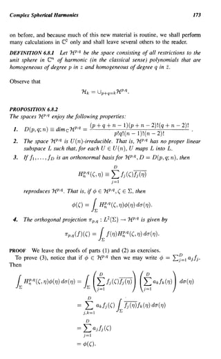
![174 A Degenerate Elliptic Boundary Value Problem
To prove (4), select 9 E L 2 (E). Then
7rp ,qg(() = 1 ~
g(1])
D
L h(1])h(() da(1])
j=1
=~ (~g(1])h(1]) da(1])) !i(()
so that 1rp,q maps £2 into 1i p ,q. By (3) it follow that 1r p,q 0 1rp,q == 1rp,q. Finally,
7rp,q is plainly self-adjoint. Thus 7rp,q is the orthogonal projection onto 1tp ,q i
In order to present the solution of the Dirichlet problem for the Laplace-
Beltrami operator 6 B, we need to define another special function. This one is
defined by means of an ordinary differential equation.
DEFINITION 6.8.3 Let a, b E IR and c > O. The linear differential equation
x( 1 - x )y" + [c - (a + b + l)x] y' - aby == 0 (6.8.3.1)
is called the hypergeometric equation.
If we divide the hypergeometric equation through by the leading factor x( 1 -
x) we see that this is an ordinary differential equation with a regular singularity
at O. It follows (see [COL]) that (6.8.3.1) has a solution of the form
(6.8.4)
where ao =1= 0 and the series converges for Ix I < 1. Let us now sketch what
transpires when the expression (6.8.4) is substituted into the differential equation
(6.8.3.1).
We find that
00 00
L ajx + - A j 1
(A + j)(A + j - 1 + c) - L ajx +j (A + j + a)(A + j + b) == 0,
A
j=O j=O
which gives the following system of equations for determining the exponent A
and the coefficients a j:
aO A(A - 1 + c) == 0
aj(A + j)(A + j - 1 + c) - aj-l(A + j - 1 + a)(A +j - 1 + b) == 0, j 2:: 1.
The first of these equations yields that either A == 0 or A == 1 - c.](https://image.slidesharecdn.com/partialdifferentialequationsandcomplexanalysis-121120212851-phpapp02/85/Partial-differential-equations-and-complex-analysis-185-320.jpg)
![Complex Spherical Harmonics 175
First consider the case A == O. We find that
(j - 1 + a) (j - 1 + b)
aj == j(j _ 1 + c) aj-I,
j == 1,2, ....
Setting ao == 1 we obtain
a(a + 1) ... (a + j - 1)b(b + 1) ... (b + j - 1)
aj == j! c(c + 1) ... (c + j - 1)
r(a + j)r(b + j)r(c)
- j!r(a)r(b)r(c + j) ,
where r is the classical gamma function (see [CCP]). Thus for A == 0 a particular
solution to (6.8.3.1) is
~ r(a + j)r(b + j)r(c) xj
y(x)=F(a,b,c;x)==~ f(a)r(b)f(c+j) . j!
Now consider the case A == 1 - c. Arguing in the same manner, if c =1=
2,3,4, ... we find (setting ao == 1 again) that a particular solution of the differ-
ential equation is given by
y ( x) == F (1 - c + a, 1 - c + b, 2 - c; x )
== x 1- c ~ r(1 - c + a + j)f(1 - c + b + j)r(2 - c) . xi
~ r(1-c+a)r(I-c+b)r(2-c+j) j!
We leave as an exercise the following statement: by checking the asymptotic
behavior of F (1 - c + a, 1 - c + b, 2 - c; x) at the origin, one may see that this
function is linearly independent from that found when A == O. The functions
F are known as the hypergeometric functions. See [ERD] for more on these
matters.
In the case that c == 2, 3, 4, ... then a modification of the above calculations
(again see [COL, p. 165]) gives rise to a solution with a logarithmic singularity
at O.
Define
s~,q(r) = r p+q F(p, q,p + q + n; r
2
) •
F(p,q,p+q+n;l)
We want to show that Sh,q is Coo on the interval (-1, 1) and continuous on
[-1, 1]. We will make use of the following classical summation tests for series.
For more on these tests, see [STR].](https://image.slidesharecdn.com/partialdifferentialequationsandcomplexanalysis-121120212851-phpapp02/85/Partial-differential-equations-and-complex-analysis-186-320.jpg)
![Complex Spherical Harmonics 177
PROOF Let b1 == 1 and bj == j - 1 for j 2:: 2. Then
Qj - 1= j (1 - a~;1 )- 1
- (J- 1) - J -
_ . . aj+l
aj
where we are using the notation of the Lemma. Then lim infj -+ oo Qj > 1 if and
only if lim infj -+00 D j > O. I
PROPOSITION 6.8.7
Take
b . ) == ~ r(a + j)r(b + j)r(c) . x
j
F(
a, ,c,x ~ f(a)r(b)f(c+j) j!
as usual. If Ixl == 1 and c > a + b then the series converges absolutely.
PROOF We want to apply Raabe's test. Thus we need to calculate the terms
Qj. Denote the absolute value of the jth summand by aj. Then, since == 1, Ixl
we have
aj+l _ (a+j)(b+j)
aj (j + 1) (c + j)
Set c == a + b + 8, where this equality defines 8 > O. Then
aj+l ab + aj + bj + j2
aj (j + 1) (a + b + 8 + j)
== 1 _ 8j + a + b + 8 + j - ab
(j + 1) (a + b + 8 + j)
-1- (1+8)j +0(1/. 2 )
- (j + 1) (a + b + 8 + j) J .
As a result,
Qj == j (1 _a~;1 )
=J
.( (1 + 8)j ( /
U+8)(a+b+8+j) +0 1 J
'2))
and lim infj -+ oo Qj == 1 + 8 > 1. Thus Raabe's test implies our result. I
It follows from the Proposition that S!:"q is continuous on [-1, 1] and Coo on
(-1, 1). We need to know when the function is in fact Coo up to the endpoints.](https://image.slidesharecdn.com/partialdifferentialequationsandcomplexanalysis-121120212851-phpapp02/85/Partial-differential-equations-and-complex-analysis-188-320.jpg)
![178 A Degenerate Elliptic Boundary Value Problem
If either p == 0 or q == 0 then the order-zero term of the hypergeometric equation
drops out. One may solve this hypergeometric equation for solutions of the form
ex>
Laj(x - l)j+,. (6.8.8)
j=O
The solutions are real analytic near 1; in particular they are smooth. On the
other hand, if both p and q are not zero, then the hypergeometric equation never
has real analytic solutions near 1 as we may learn by substituting (6.8.8) into
the differential equation. In fact the solutions are never where n is the en,
dimension of the complex space that we are studying.
REMARKS Gauss found that
. r(c)r(c-a-b)
x-+l
hm_F(a,b,c;x)=q c - a )f( c- b)'
Also, one may substitute the function
y= { (u-x)f.-I¢(u)du,
J[O,l]
where ~ is a constant to be selected, into the hypergeometric equation. Some
calculations, together with standard uniqueness theorems for ordinary differential
equations, lead to the formula
F(a b C' x) == r(c)
, , , r(b)r(a)
10
1
t b- I (1 - t)a-b-l (1 - xt)-a dt
for 0 < x < 1. It is easy to see from this formula that F cannot be analytically
continued past 1. I
As a consequence of our last proposition,
SM (r) = rp+q F(p, q,p + q + n; r 2 )
n F(p,q,p+q+n;l)
is well defined and Coo when 0 ~ r < 1.
THEOREM 6.8.9
Let f E 1t p ,q. Then the solution of the Dirichlet problem
6BU == 0 on B
{ U == f on 8B == E
is given by
for ( E L: and 0 ~ r ~ 1.](https://image.slidesharecdn.com/partialdifferentialequationsandcomplexanalysis-121120212851-phpapp02/85/Partial-differential-equations-and-complex-analysis-189-320.jpg)
![Complex Spherical Harmonics 179
PROOF To simplify the calculations, we shall prove the theorem only in di-
mension n == 2.
Let F o(z) == zf z1
and fo == F oIaB· Then the ordinary Laplacian
6=4(~+~)
{)ZI{)ZI {)Z2{)Z2
annihilates Fo. Recall that 1i p ,q is irreducible for U(2). This means that
{f 0 a }aEU(2) spans all of 1t p ,q (for if it did not it would generate a non-
trivial invariant subspace, and these do not exist by definition of irreducibility).
Furthermore, 6 B commutes with U(2) so if we prove the assertion for fo, Fo
then the full result follows.
For z E B we set r == Izl. Then r 2 == ZlZI + Z2Z2. We will seek a solution
of our Dirichlet problem of the form
u(z) == g( r 2 )zf Z2 q.
Recall that
4 n {)2
6 B == - + 1 (1 -lzI2) " (8·· -
n ~ 1,)
z·z·) - - .
1,) {)z.{)z.
i,j=1 1, )
We calculate 6BU.
Now
{)
{)z. u == Zjg ,(r 2) [zlP z2 + 9 (r 2) zlP
-q] ( -q -1) U2j
q Z2
~
)
and
Therefore
L2 {)2 u
oz.oz =
{2
L [g"(r 2 )l ziI 2 + g'(r 2 )] zfzi
}+ g'(r )pziZi + g'(r )qzfzi
2 2
i=1 1, Z i=1
== zf z1 [g"(r 2)r2 + (2 + p + q)g'(r 2)] .
By a similar calculation we find that
2 {)2 u
L
i,j=1
ZiZj~
ZiZj
= zfzi [r 4 gll (r 2 ) + (p + q + 1)r2 g'(r 2 ) + pqg(r 2 )] •](https://image.slidesharecdn.com/partialdifferentialequationsandcomplexanalysis-121120212851-phpapp02/85/Partial-differential-equations-and-complex-analysis-190-320.jpg)
![180 A Degenerate Elliptic Boundary Value Problem
Substituting these two calculations into the equation 6 Bu == 0 (and remember-
ing that n == 2), we find that
o == 6 Bu == -4 (1 - r 2)zfzi [g"(r 2)r 2 + (2 + p + q)g'(r 2)]
2
+1
4
- - 2 (l-r2)zfzi[g"(r2)r4+(p+q+l)r2g'(r2)+pqg(r2)]
+1
= 2 ~ 1(1 - 2 2 2
r 2)zf zf {r (1 - r )g" (r )
+ [(p + q + 2) - (p + q + l)r 2] g'(r 2) - pq g(r 2)}.
Therefore, if a solution of our Dirichlet problem of the form of u(z) == g(r2)zfzi
exists, then 9 must satisfy the following ordinary differential equation:
We may bring the essential nature of this equation to the surface with the changes
of variables t == r 2 , a == p, b == q, C == P + q + 2. Then the equation becomes
t (1 - t) g" + [c - (a + b + 1)t] g' - ab 9 == O.
This, of course, is a hypergeometric equation. Since u is the solution of an
elliptic problem, it must be Coo on the interior. Thus 9 must be Coo on [0, 1).
Given the solutions that we have found of the hypergeometric equation, we
conclude that
g(t) == F(p, q,p + q + n; t).
Consequently,
F(p,q,p+q+n;r2) p_q
u () ==
z z z
F(p, q, p + q + n; 1) 1 2
== S~,q(r)rp+q f((). I
THEOREM 6.8.10
~ r < 1 and 1], ( E aBo Then the Poisson-Szego kernel for the ball
Let 0
B ~ en is given by the formula
00
P(r1],() == L S~,q(r)H~,q(1J,().
p,q=O
PROOF Recall that if 9 E C(aB), then
G(z) == { JaB P(z, ()g(() du(() on B
g(z) on 8B](https://image.slidesharecdn.com/partialdifferentialequationsandcomplexanalysis-121120212851-phpapp02/85/Partial-differential-equations-and-complex-analysis-191-320.jpg)
![Complex Spherical Harmonics 181
solves the Dirichlet problem for 6 B with data g. Recall also that Hh,q (1], () is
the zonal harmonic for 1i p,q.
Let us first prove that the series in the statement of the theorem converges.
An argument similar to the one we gave for real spherical harmonics shows that
Here D(p, q; n) is the dimension of 1ip ,q. Clearly,
D( . n) < dim 1ip+q == (2n + (p + q) - 1) _ (2n + (p + q) - 3)
p,q, - 2n
p+q p + q- 2
~ C . (p + q + 1)2n.
Recall that
Sp,q(r) = r p +q F(p, q,p + q + n; r 2 )
n F(p,q,p+q+n;l)
and observe that F(p, q, p + q + n; r 2 ) is an increasing function of r. Thus
Putting together all of our estimates, we find that
Summing on p and q for 0 ~ r < 1 we see that our series converges absolutely.
It remains to show that the sum of the series is actually the Poisson-Szego
kernel. What we will in fact show is that for 1] E 8B and 0 < r < 1 we have
for every f E C(8B). But we already know that this identity holds for f E 1ip ,q.
Finite linear combinations of Up,q 1i p ,q are dense in C( 8B). Hence the result
follows. I
Now we return to the question that has motivated all of our work. Namely, we
want to understand the lack of boundary regularity for the Dirichlet problem for
the Laplace-Beltrami operator on the ball. As a preliminary, we must introduce
a new piece of terminology.
DEFINITION 6.8.11 Let U ~ en be an open set and suppose that f is a
continuous function defined on U. We say that f is pluriharmonic on U if for](https://image.slidesharecdn.com/partialdifferentialequationsandcomplexanalysis-121120212851-phpapp02/85/Partial-differential-equations-and-complex-analysis-192-320.jpg)
![182 A Degenerate Elliptic Boundary Value Problem
every a E U and every bEen, it holds that the function
(~f(a+(b)
is harmonic on the open set (in C) of those ( such that a + (b E U.
A function is pluriharmonic if and only if it is harmonic in the classical sense
on every complex line ( ~ a + (b. Pluriharmonic functions arise naturally
because they are (locally) the real parts of holomorphic functions of several
complex variables (see [KRl, Ch. 2] for a detailed treatment of these matters).
Remark that a C 2 function v is pluriharmonic if and only if we have
2
(8 /8z j 8z k )v == 0 for all j, k. In the notation of differential forms, this condi-
tion is conveniently written as 8av == o.
Now we have
THEOREM 6.8.12
Let f E CX(8B). Consider the Dirichlet problem
6BU == 0 on B
{ ul aB == f on 8B.
Suppose that the solution u of this problem (given in Proposition 6.5.2) lies in
COO(B). Then u must be of the form
That is, u must be pluriharmonic. The converse statement holds as well: if f
is the boundary function of a pluriharmonic function u that is continuous on 13
and if f is Coo on the boundary, then U E Coo (B).
PROOF Now let v E C(B) and suppose that v is piuriharmonic on B. Let
vlaB == f· Then the solution to the Dirichlet problem for 6 B with data f is in
fact the function v (exercise). But then v is also the ordinary Poisson integral
of f. Thus if f E COO(8B) then v E COO(B). This proves the converse (the
least interesting) direction of the theorem.
For the forward direction, let f E Coo (8B) and suppose that the solution u
of the Dirichlet problem for 6 B with data f is Coo on B. We write
f == LYp,q,
p.q
where each ~,q E 1i p ,q. We proved above that
p,q](https://image.slidesharecdn.com/partialdifferentialequationsandcomplexanalysis-121120212851-phpapp02/85/Partial-differential-equations-and-complex-analysis-193-320.jpg)
![Complex Spherical Harmonics 183
and also that the solution to the Dirichlet problem for 6 B is given by
u(r7J) J P(r7J,()f(()da(()
L L JS~'·q' (r)H~',q' (71, ()Yp,q(() da(()
p',q' p,q
(ortho~nality) L s~,q (r) JH~,q (71, ()Yp,q( () da( ()
p,q
L S~,q(r)Yp,q(1J).
p,q
Therefore if P f == u is smooth on 13 then we may define for each p, q the
function
Qp,q(r) = { (P J)(r()Yp,q(() da(()
JaB
== S~,q(r)IIYp,qIl2.
Thus if P f is Coo up to the boundary then, by differentiation under the integral
sign, Qp,q (r) is Coo up to r == 1. But recall that
Sp,q(r) = r p+q F(p, q, p + q + n; r 2 )
n F(p,q,p+q+n; 1)
is smooth at r == 1 if and only if either p == 0 or q == O. So the only nonvanishing
terms in the expansion of f are elements of 1iP 'o or 1t0 ,q. That is what we
wanted to prove. I
We leave it to the reader to prove the refined statement that if a solution u to
the Dirichlet problem is cn
up to the closure, then u must be pluriharmonic.
The analysis of the Poisson-Szego kernel using bigraded spherical harmonics
is due to G. B. Folland [FOL]. We thank Folland for useful conversations and
correspondence regarding this material.
An analysis of boundary regularity for the Dirichlet problem of the Laplace-
Beltrami operator on strongly pseudoconvex domains was begun in [GRL].
Interestingly, these authors uncovered a difference between the case of dimen-
sion 2 and the case of dimensions 3 and higher.](https://image.slidesharecdn.com/partialdifferentialequationsandcomplexanalysis-121120212851-phpapp02/85/Partial-differential-equations-and-complex-analysis-194-320.jpg)
![7
The a-Neumann Problem
Introductory Remarks
The a-Neumann problem is a generalization to several complex variables of the
Cauchy-Riemann equations of one complex variable. While the groundwork
for this problem was laid by D. C. Spencer, Charles Morrey, P. Conner, and
others, it was J. J. Kohn [KOHl] who tamed the problem. It is the key to many
of the important techniques of the function theory of several complex variables.
The a-Neumann problem was also one of the first non-elliptic problems for
which a regularity theory was established. Whereas in an elliptic problem of or-
der m we have learned that the solution is m degrees smoother than the data, the
a-Neumann problem does not exhibit the maximal degree of smoothing. Indeed
the a-Neumann problem is subelliptic rather than elliptic; roughly speaking,
this means that the solution gains a predictable number of derivatives, but that
number is less than the degree of the partial differential operator in question.
Subelliptic regularity was quite unexpected in the early 1960s when it was
first discovered (see [KOH 1]). It cannot be treated by a naive application of
the theory of pseudodifferential operators or by other classical techniques. The
monograph [GRS] describes a special calculus of pseudodifferential operators
designed for the study of the a-Neumann problem on an important special class
of domains; indeed, it is the same special class that we shall study here.
The method that we present here is not Kohn's original, which is rather com-
plicated, but is a simpler method, called elliptic regularization, that he developed
later in collaboration with Nirenberg (see [K02], [FOK] and references therein).
The monograph [FOK] is the canonical reference for matters related to the a-
Neumann problem. However, the presentation there is perhaps too complicated
for our purposes, since it is in the setting of an arbitarary metric structure on an
almost complex manifold. In an effort to maintain simplicity, we shall formu-
late and solve the a-Neumann problem only on a smoothly bounded strongly
pseudoconvex domain in en. We do follow the basic steps in [FOK], but by
specializing we can provide considerably more detail and context.](https://image.slidesharecdn.com/partialdifferentialequationsandcomplexanalysis-121120212851-phpapp02/85/Partial-differential-equations-and-complex-analysis-195-320.jpg)
![Introduction to Hermitian Analysis 185
Those interested in the most general setting for the a-Neumann problem will,
after reading the material here, be well prepared to consult [FOK] and other
more recent sources (see, for instance, [RAN] and [CATl]-[CAT3]) on the a-
Neumann problem.
7.1 Introduction to Hermitian Analysis
As previously mentioned, we shall be working strictly on domains in Cn . We
may thus bypass a certain amount of formalism by relying on the standard
coordinates in space.
If P E Cn ~ IR.2n then the tangent space to IR.2n at P is spanned by
8 8 8 8
8Xl ' 8Yl ' ... , 8x n ' 8Yn .
It clearly has (real) dimension 2n. We set
8 1[8 .8]
---
8z j - 2
--l-
8xj 8Yj
8 = 2 + .8]
8zj
1[8 8xj z8Yj .
Then we let Tl,o denote the complex linear space spanned by
and ro,l == Tl,O denote the complex linear space spanned by
8 8
8z , ••• , 8z .
l n
The complexified tangent space is then
It obviously has complex dimension 2n. The complexified tangent space is, in a
natural sense, the tensor product of the real tangent space with C. However, we
shall have no use for this formalism (see [WEL] for more on this point of view).
There is associated to the complexified tangent space a complexified cotangent
space. We set
dZ j== dXj + idYj
dZj == dXj - idYj.](https://image.slidesharecdn.com/partialdifferentialequationsandcomplexanalysis-121120212851-phpapp02/85/Partial-differential-equations-and-complex-analysis-196-320.jpg)
![186 The a-Neumann Problem
A trivial calculation shows that
dZj'8~j)=1, dz j , 8~j ) = 0,
dzj , 8~j ) = 0, dzj , 8~j ) = 1.
If a == (aI, ... , as) is a multiindex, then we set
and
dz a == dZal 1 dZa2 1 ... 1 dzas .
In this context the magnitude of the multiindex is lal == s. (The use of mul-
tiindices here is rather at odds with some earlier uses in this book, but should
lead to no confusion.) Then 1 p,q denotes the space of forms of the type
W == L aa(3dz a 1 dz(3.
lal=p,I(3I=q
It is an exercise in linear algebra to see that if 1 r denotes the space of all
classical (real variable) r- forms on en ~ ]R2n, then
IT = (J) Ip,q.
p+q=r
Next we tum to the exterior derivative. Let
W == L aa,(3dz a 1 dz(3
a,(3
be a differential form. The exterior derivative d may be written as d == 8 + 8,
where
8w = ' " ~ 8aO!,{3 dz· / dzO! / dz{3
L...J L...J 8z. J
a,(3 j=1 J
and
8w = Lt 8;; :{3 dZ j / dzO! / dz{3.
a,(3 j=1 J
Clearly,
_ Ip,q IP,q+l
and 8: -+ .
Since
0== d2 == (8+ 8)(8+ 8),](https://image.slidesharecdn.com/partialdifferentialequationsandcomplexanalysis-121120212851-phpapp02/85/Partial-differential-equations-and-complex-analysis-197-320.jpg)
![190 The a-Neumann Problem
Thus a necessary condition for the equation (7.2.1) to have a solution is that
aI == O. This point bears a moment's discussion.
In C l , the Cauchy-Riemann equations for C l functions v == ~ + iT) and
I == u + iv can be written either as
~ (8~
2 8x
_8T)) ==
8y
u and ~ (8T) + 8~) == v
2 8x 8y
or as
8v == I
8z .
In either notation, the number of unknown functions is in balance with the
number of equations. However, in dimensions two and greater the situation is
different. Write 1== Ildz l + ... + Indzn. Then our system (7.2.1) is
8v
-8- == Ij, j == 1, ... , n,
Zj
and the number of equations (n) exceeds the number of unknown functions
( I). Passing to real notation results in no improvement. We call such a system
overdetermined. Algebraic considerations (or dimension) suggest that some
compatibility conditions will be needed on the data in order for the system to
be solvable. And indeed that is what we have discovered. (A formal theory of
overdetermined systems of partial differential equations has been developed by
D. C. Spencer; see for instance [SPE].)
There is also a problem with uniqueness for solutions of (7.2.1). For if u is
one solution to this equation and h is any holomorphic function, then u + h is
also a solution. In order to obtain a workable theory for this partial differential
equation, we shall need a canonical method for choosing a "good" solution. For
this we shall exploit the metric structure introduced in the last section. First let
us see that the a
operator is elliptic in a natural sense. When we are dealing
with an operator onforms, a certain amount of formalism is ultimately necessary.
However, the a
operator acting on functions may be thought of as an n-tuple
az az
comprised of the operators 8/ l , ••. ,8/ n . Each of these is plainly elliptic
on a suitable copy of C, and they span all directions. Hence so is the operator
a itself elliptic.
Now we tum to the question of ellipticity on forms. Let 0 ~ be a domain. cn
Think of E == EP,q as the vector bundle of (p, q) covectors over O. Then a
differential form w of type (p, q) is a section of this vector bundle: we write
W E r(E). Letting F == EP,q+l, we then have
a:r(E) ~ r(F).
Fix Z E O. The symbol of aassigns to each covector T) at Z a linear mapping](https://image.slidesharecdn.com/partialdifferentialequationsandcomplexanalysis-121120212851-phpapp02/85/Partial-differential-equations-and-complex-analysis-201-320.jpg)
![The Formalism of the [) Problem 191
This is done as follows: It is elementary to construct a scalar-valued function
p such that p( z) == 0 and dp( z) == 7] Uust use Tayor series-or even the funda-
mental theorem of calculus). If J.L E E z, we let jj be a local section of E such
that jj( z) == J.L Uust work in a neighborhood of z over which E is trivial). We
define
a([), 7])J.L == [)(p. jj) Iz·
The reader should check that for a classical first-order partial differential op-
erator acting on functions, this definition is consistent with the one discussed
in Chapters 3 and 4. Of course, in the case of functions, the vector bundles E
and F are just 0 x C.
With this definition of symbol, we now explicitly calculate the symbol of 8.
With 7], p, J.L as in the definition we have
Here ITo, 1 is the projection of a I-form into 10,1. We see that
a ([), 7] ) ( . ) == ITo, 17] 1 ( . ). (7.2.2)
Now, in the present g~neral setting, an operator is said to be elliptic if the
complex
a(8,TJ) F
O ---+ E Z ---+ Z
is exact, that is, if a([), 7]) is injective. In the case that p == 0, q == 1, that is,
when [) is acting on functions, it is then clear that [) is elliptic. When [) is acting
on forms of higher order, we must speak of ellipticity of a complex. Namely, a
sequence
r(E) ~ r(F) ~ r(G)
is called elliptic if the induced sequence
a(Dt,TJ) F a(D2 ,TJ) G
Ez ---+ Z ---+ Z
is exact at Fz-that is, if the kernel of the second mapping equals the image of
the first. We invite the reader to check that the [) complex
is elliptic (or see [FOK, pp. 10-11] for further details).
Let us now discuss the formal adjoint of the 8 operator. We work on a
domain 0 ~ Cn . If we think of [) : Ip,q ---+ Ip,q+l then the formal adjoint
{) : I~,q+ 1 ---+ I~,q is defined by the relation](https://image.slidesharecdn.com/partialdifferentialequationsandcomplexanalysis-121120212851-phpapp02/85/Partial-differential-equations-and-complex-analysis-202-320.jpg)
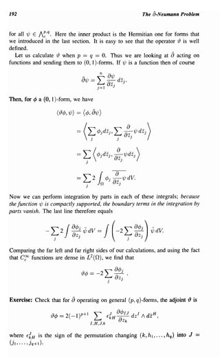
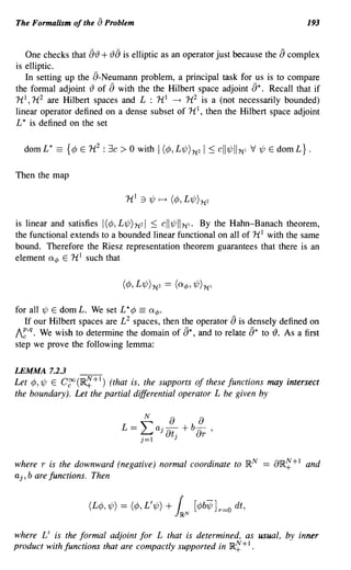
![194 The a-Neumann Problem
PROOF Now
(L¢, 1/;) =
1 (2: lR + + 1
N
N
,
)=1
fJ¢
aj ~
ut)·
fJ¢)
+ b~ Ur
-
1/; dt dr
== ~
~1N
.
)=1
~N+l
+
fJ¢-
aj~1/;dtdr
utj
+ 1 jRN+l
+
fJ¢-
b~1/Jdtdr
ur
=- f., J~N+l ¢J ",0
j=1
r
mo.+)
ut·
(aj:¢) dt dr + r
J~N
mo."
¢Jb1fIO
r=-oo
dt
- JjRN+l ¢J ur (b1f) dt dr.
r ~
+
Notice that in the first group of integrals we have used the fact that the tj
directions are tangential, together with the compact support of 1/J, to see that no
boundary terms result from the integrations by parts. Now the last line is
r N
JlR+ +1
¢J [- f., ",0
,ut)'
(aj¢) - ~ (b¢)]
ur
dt dr + r
JjRN
[¢Jb1f]
r
=0 dt
)=1
-= (¢J, L' ¢) + r
JlR N
[¢Jb1flr=o dt.
That completes the proof. I
A simple computation shows that
N N
a(L, 2: 7]j dtj + 7]r dr ) == 2: 7]jaj (t, r) + 7]r b(t, r).
j=1 j=1
In particular, a (L, dr) == b and the integral from our lemma satisfies
r
JlRN
[¢Jb1f]
r
=0 dt = r
JalRN+1
(cy( L, dr )¢J, ¢) dt.
+
The arguments that we have presented are easily adapted from the half-space
to a smoothly bounded domain (just use local boundary coordinate patches).
The result is that
(Lf,g) = (J,L'g) + r
Jan
(cy(L,dr)f,g).
The arguments also are easily applied to partial differential operators on a vector](https://image.slidesharecdn.com/partialdifferentialequationsandcomplexanalysis-121120212851-phpapp02/85/Partial-differential-equations-and-complex-analysis-205-320.jpg)
![198 The a-Neumann Problem
Exercise: Show that U is dense both in V and in H. (Hint: Use the fact that
T is self-adjoint.)
We intend to apply the Friedrichs lemma to the 8-Neumann problem. To this
end, we introduce the following notation:
1. Let H == HC,q == {(p, q)-forms with £2 coefficients on o}.
2. Let Q( ¢, 1/;) == (8¢, 81/;) + (r13¢, 'l31/;) + (¢, 1/;).
3. Let V == vp,q == the closure of vp,q in the Q-topology.
Now we have to do some formal checking: There is a natural continuous
inclusion of vp,q in HC,q. We will see that this induces an inclusion of vp,q
in HC,q.
Let {¢n} be a Q-Cauchy sequence in vp,q. By definition of Q, we see
that {¢n}, {'l3¢n}, and {8¢n} are Cauchy sequences in HC,q (i.e., in the £2
topology). Let ¢ be the £2 limit of {¢n}. When interpreted in the weak or
distribution sense, 8 and 'l3 are closed operators. Hence we have
and
If ¢ == 0 in £2 then
Q(¢,¢) == limQ(¢n,¢n) == lim [(¢n,¢n)
n n---+oo
+ (8¢n,8¢n) + ('l3¢n,'l3¢n)]
== (¢, ¢) + (8¢,8¢) + ('l3¢, 'l3¢) == O.
Therefore ¢n ----+ 0 in the Q-topology. It follows that the inclusion vp,q ~ HC,q
extends to the inclusion vp,q ~ HC,q.
Now we may apply the Friedrichs theorem to obtain a (canonical) self-adjoint
map
F : dom F ( ~ vp,q) -t H6,q
dense
such that
Q( ¢, 1/J) == (F¢,1/;)
for all ¢ E dom F, '¢ E V. Now we need to identify F and determine its
domain.
Set
p,q -
v~,q == I n dom {)* == {p E vp,q : supp p is compact}.
c](https://image.slidesharecdn.com/partialdifferentialequationsandcomplexanalysis-121120212851-phpapp02/85/Partial-differential-equations-and-complex-analysis-209-320.jpg)
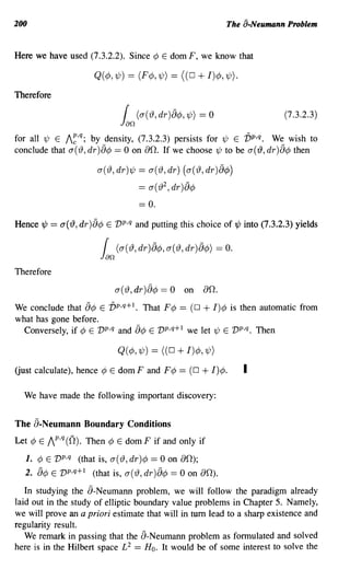
![The Main Estimate 201
problem in other Hilbert spaces, such as the Sobolev space HS. The groundwork
for studying those Hilbert spaces has been laid in [BO 1]. However, as of this
writing, it is not clear what the Neumann boundary conditions should be in that
context.
7.4 The Main Estimate
If Q E Hg,q, then the construction of the operator F guarantees the existence of
a unique ¢ E vp,q such that F ¢ == Q. We are interested in the regularity up to
the boundary of this solution ¢. If we had a classical Garding type, or coercive,
inequality
Q(¢, ¢) 2: cll¢IIT,
then it would be straightforward to prove the desired estimates. We do not have
such an inequality, but will find a substitute that will do the job.
LEMMA 7.4.1
Let 0 ~ enbe a smoothly bounded domain with defining function r: 0 = {z E
en : r(z) < O} and IVrl == 1 on 00. Then
1. If ¢ E 10,1, then ¢ E VO,I if and only if Lj(ar/aZj)¢j == 0 on 80.
2.
on 00.
3. If f,9 E Coo(O) then we have
where 'Y is the volume element.
4.
(---: L ian fg-j
1)
2z
n
.
J
or
8z
da == L.
J
1(8
0.
f
-g + f~
8z j
0- )
8zj
'Y.
5. The analog of (4) with 0/ aZj replaced by 0/ aZj.](https://image.slidesharecdn.com/partialdifferentialequationsandcomplexanalysis-121120212851-phpapp02/85/Partial-differential-equations-and-complex-analysis-212-320.jpg)
![202 The a-Neumann Problem
PROOF (1) This is just definition checking: Let p E 00, and let r be a defining
function with Idrl == 1 on 00,. Of course r(p) == O. Let ¢ == 2:7=1 ¢idzi. Then
¢ E V O,l if and only if
o == O"('19,dr)¢!p
== 19(r¢)l p
== ('19r )p(¢p)
=- L
n
j=l
8:
a
J
(p)¢>j(p)o
If we apply Idr to both sides of the equation in the statement of (2), then
the result is or/aZ j . 1 == or/aZ j ·1. Resuft (2) follows.
To prove (3), we calculate that
d [jg (- ;J n dZ I / dZ I / 0 0 0 ~ / 0 •• / dZ n / dZn ]
= [8~j (fg) (- ;i) n dZ j / dZ I / dZ I / • •• / ~ / 0 •• / dZn / dZ n ]
( 1)
== ---;-
2~
n ( of
- g + f~ ) 1·
aZ j
0-
aZ j
To prove (4), we apply Stokes's theorem to (3). Thus
L lEi fg (1 )n dZ
n { - 2i I / dZ I / • .. /
. . -. .
dZ j / ... / dZ n / dZn
j=l an
== L 1(of ,g+f ag 'Yo
n
n
j=l
-a 0-) ZJ ZJ
Now we use (2) and the fact that *dr == dO" to see that the left side is equal to
(---;- L 1 f9- dO".
1)
2~
or
8z
n n
j=1 an j
I](https://image.slidesharecdn.com/partialdifferentialequationsandcomplexanalysis-121120212851-phpapp02/85/Partial-differential-equations-and-complex-analysis-213-320.jpg)
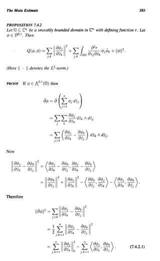
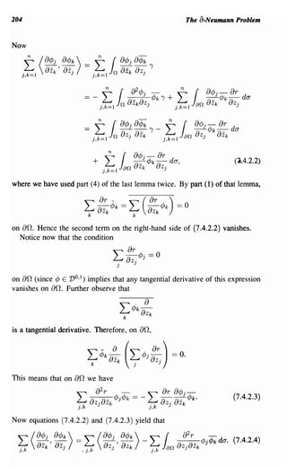
![The Main Estimate 205
Substituting (7.4.2.4) into (7.4.2.1) yields that
As a result,
That completes the proof. I
DEFINITION 7.4.3 Let f2 == {z E en :
r(z) < O} be a smoothly bounded
domain. If p E of2 then let a be a complex tangent vector to of2 at p, i.e.,
n or
L oz- (p)aj = O.
j=1 J
The Levi form at p is defined to be the quadratic form
We say that f2 is pseudoconvex at p if L p is positive semidefinite on the space
of complex tangent vectors. We say that f2 is strongly pseudoconvex at p if
L p is positive definite on the space of complex tangent vectors. We say that
f2 is pseudoconvex (resp. strongly pseudoconvex) if every boundary point is
pseudoconvex (resp. strongly pseudoconvex)·.
For emphasis, a pseudoconvex domain is sometimes called weakly pseudocon-
vex.
The geometric meaning of strong pseudoconvexity does not lie near the sur-
face. It is a biholomorphically invariant version of strong convexity (which
concept is not biholomorphically invariant). A detailed discussion of pseudo-
convexity and strong pseudoconvexity appears in [KR 1]. In particular, it is
proved in that reference that if p is a point of strong pseudoconvexity, then
there is a biholomorphic change of coordinates in a neighborhood of p so that
p becomes strongly convex.](https://image.slidesharecdn.com/partialdifferentialequationsandcomplexanalysis-121120212851-phpapp02/85/Partial-differential-equations-and-complex-analysis-216-320.jpg)
![The Main Estimate 207
Exercise: Show that for 1/J E /~,q (U), U ceO, we have Q(1/J, 1/J) 2: c 1I1/J II I
(hint: integrate by parts). Then on /~,q (U) we have a classical coercive esti-
mate. The lack of full regularity in some directions for the a-Neumann problem
is due to the complex geometry of the boundary.
Exercise: Show that on any smoothly bounded domain 0 the expression E( . )
satisfies
E(¢) ~ C· 1I¢lIi
for all ¢ E 1 p,q (0), but that in general there is no constant C' > 0 such that
E(¢) 2: C'II¢lli
for all ¢ E /P,q (0).
Now we are ready to formulate the main theorem of this chapter. Recall that,
by construction, the equation F¢ == Q admits a unique solution ¢ E dom (F)
for every Q E Hg,q (0).
THEOREM 7.4.7 THE MAIN ESTIMATE
Let n ~ enbe a smoothly bounded domain. Assume that the basic estimate
holds for elements of vp,q (0). For Q E Hg,q, we let ¢ denote the unique
solution to the equation F¢ == Q. Then we have:
1. If W is a relatively open subset of 0 and if Qlw E /P,q(W), then
¢w E /P,q(W).
2. Let P, PI be smooth functions with supp P ~ supp PI ~ Wand PI == 1 on
supp p. Then:
(a) If W n ao == 0 then Vs 2: 0 there is a constant Cs > 0 (depending
on P, PI but independent of Q) such that
(b) If W n ao 1= 0 then Vs 2: 0 there exists a constant Cs 2:: 0 such that
REMARK Observe that (1) states that F is hypoelliptic. Statement (2a) asserts
that, in the interior of 0, the operator F enjoys the regularity of a strongly
elliptic operator. That is, F is of order 2 and the solution of F ¢ == Q exhibits
a gain of two derivatives.
On the other hand, (2b) states that at the boundary F enjoys only subelliptic
regularity-the solution enjoys a gain of only one derivative. Examples ([FOK],
[GRE], [KR4]) show that this estimate is sharp. I](https://image.slidesharecdn.com/partialdifferentialequationsandcomplexanalysis-121120212851-phpapp02/85/Partial-differential-equations-and-complex-analysis-218-320.jpg)
![208 The a.Neumann Problem
The proof of the Main Estimate is quite elaborate and will take up most of
the remainder of the chapter. We will begin by building up some technical
machinery. Then we show how to derive (2a) from the results of Chapter 4.
Next, and what is of most interest, we study the boundary estimate. Of course (1)
follows from (2a), (2b). All the hard work goes into proving statement 2(b). The
tradeoff between existence and regularity is rather delicate in this context. To
address this issue we shall use the technique, developed by Kohn and Nirenberg,
of elliptic regularization (see [KON2]).
Before we end the section, we wish to stress that part (2a) is the least in-
teresting of all the parts of the Main Estimate. For notice that if ¢, 1j; E I~,q
then
(F¢,1j;) == ((0 + I)¢, 1j;) .
Now 0 +I is elliptic, so the regularity statement follows from Theorem 4.2.4.
7.5 Special Boundary Charts, Finite Differences, and Other Technical
Matters
The proof of the Main Estimate has at its heart a number of sophisticated
applications of the method of integration by parts. As a preliminary exercise we
record here some elementary but useful facts that will be used along the way.
LEMMA 7.5.1
For every t > 0 there is a K > 0 such that for any a, b E IR we have
ab:::; ta 2 + Kb 2 •
PROOF Recall that 2aj3 :::; a 2 + j32 for all a, j3 E lit Hence
2ab = 2 ( ~a) (~b)
< 2ta2 + ~b2.
- 2t
Thus K == 1/4t does the job. I
LEMMA 7.5.2
If D 1 , D 2 are partial differential operators of degrees k 1 , k 2 , respectively, then
has degree not exceeding k 1 + k2 - 1.](https://image.slidesharecdn.com/partialdifferentialequationsandcomplexanalysis-121120212851-phpapp02/85/Partial-differential-equations-and-complex-analysis-219-320.jpg)
![210 The a-Neumann Problem
Then v is normal to U nao. Complete v to an orthonormal basis £1, ... , £n-l , v
for T~o(O),P E U. The canonical dual basis Wl, ... ,W n E /1'°(0) satisfies
Wn == V2ar. __
Check that £1, ... £n-l, £1, ... , £n-l, 1m v form a basis for Tq(aO), q E 00.
On a special boundary chart the a-Neumann boundary conditions can be easily
expressed in terms of coordinates:
LEMMA 7.5.4
If U is a special boundary chart and
¢ == L¢ I Jw
I
1 wJ
I,J
on U then <P E vP,q if and only if ¢ E /P,q (0) and <PI J = 0 on 00 whenever
n E J.
PROOF Exercise. This is just definition chasing (or see [FOK, p. 33]). I
Finite Differences
In learning about the calculus of finite differences we shall use IRN as our setting.
If U is a function on IRN , j E {I, ... , N}, and h E 1R, then we define
. 1 [
.6~U(Xl, ... ,XN) = 2ih U(Xl, ... ,Xj-l,Xj+h,xj+l, ... ,XN)
- u(xJ, ... ,Xj-J,Xj - h,Xj+I, ... ,XN)].
Also if (3 == ((31, ... , (3 N) is a multiindex and
H = (h jk ) J=I"."N
k=l"",{3j
is an array of real numbers then we define
Here the symbol TI is to be interpreted as a composition of the .6 operators.](https://image.slidesharecdn.com/partialdifferentialequationsandcomplexanalysis-121120212851-phpapp02/85/Partial-differential-equations-and-complex-analysis-221-320.jpg)
![Special Boundary Charts, Finite Differences, and Other Technical Matters 211
Example: Let N == 1, (3 == (2), and H == (h, h) with h > O. If u is a function
then
~~U(X) == 6h (6h u (X))
== 6h (u(x + h) - u(x - h))
== u(x + 2h) + u(x - 2h) - 2u(x).
This is a standard second difference operator such as one encounters in [ZYG]
(see also Chapters 4 and 5). 0
A comprehensive consideration of finite difference operators may be found
in [KR2]. We shall limit ourselves here to a few special facts.
LEMMA 7.5.5
If u E L 2 (IR N ) then
(6{ U r (~) = - Sin~~j) u(~).
Here --denotes the standard Fourier transform.
PROOF We calculate that
(6~Ur (~) = 2:h JeiX~[u(Xl, .•. ,Xj +h, ... ,XN)
- U(Xl, ... ,Xj -h, ... ,XN)]dx
= 2:h [e -ih~j - eih~j] u(~)
= _ Sin~~j)u(~). I
Notice that
as h ---+ o.
LEMMA 7.5.6
Let u E HS'C~N),/3 a multiindex, 1/31 == s. Ifr:S s' - s then for any H we
have
(Here the norms are Sobolev space norms.)](https://image.slidesharecdn.com/partialdifferentialequationsandcomplexanalysis-121120212851-phpapp02/85/Partial-differential-equations-and-complex-analysis-222-320.jpg)
![212 The a-Neumann Problem
PROOF We calculate that
116~ ull; = 1(1 + 1~12r [(6~uf (~)12 d~
= 1 + 1~12r f1 fi
(1 I ::kk~j 12IU(~)12~
sin
N
:s 1(1 + 1~12r II I~j 1 lu(~)12 d~
213J
j=1
= 1(1 + 1~12r [(D13 u f (~)12 d~
== IID/3ull;. I
LEMMA 7.5.7 SCHUR
Let (X, /-L), (Y, v) be measure spaces. Let K : X x Y ~ C be a jointly
measurable function such that
1 IK(x, y)1 dJ-L(x) ::::; c,
uniformly in y E Y, and
1 IK(x, y)1 dv(y) ::::; c,
uniformly in x EX. Then the operator
f f-7 1 K(x, y)f(y) dv(y)
maps LP(Y, v) to LP(X, /-L), 1 :s p :s 00.
PROOF For p == 00 the assertion is obvious. For 1 :s p < 00, use Jensen's
inequality from measure theory (or the generalized Marcinkiewicz inequality,
for which see [STSI]). I
We now introduce an important analytic tool that is useful in studying smooth-
ness of functions. We saw a version of it earlier in Chapter 5.
DEFINITION 7.5.8 The Bessel potential of order r is defined by the Fourier
analytic expression
where ¢ E C~. This operation extends to Hr in a natural way.
Observe that ¢ E Hr if and only if Ar¢ E L 2 (= HO). Notice also that
Ar : H t ----+ H t - r for any t, r E Ilt](https://image.slidesharecdn.com/partialdifferentialequationsandcomplexanalysis-121120212851-phpapp02/85/Partial-differential-equations-and-complex-analysis-223-320.jpg)
![Special Boundary Charts, Finite Differences, and Other Technical Matters 213
LEMMA 7.5.9
If a E C~ (lR N ) and r :::; s' - s, then for all u E H s' -1 and multiindices f3 with
1f31 == s, we have
that is, [a, 6~] behaves like an operator of order s - 1.
PROOF First we consider the case If31 == 1. We want to show that
II [a, 6{]ull r ;S Iluli r
for any r and any u E H s' ,s' ~ r. Using Bessel potentials, this inequality is
seen to be equivalent to
Now, if F denotes the Fourier transform then
(7.5.9.1 )
where
K(C ) ==
~, 77
(1 +
+
1
2
/771 ) r/2 [sin(h 77 j ) _
1~12
0
h
Sin(h~j)] --(
h a 77
_ C)
~.
In fact, let us do the calculation that justifies this assertion: According to the
definition of the Bessel potential we have
Next,
= a* (L.{A-rvf ("1) + Sin~17j) (a* (A-rv)) ("1)
= - (a * [Sin~ OJ) (1 +I 0
2)-r/2
1 (
v 0 )]) ("1)
+ Sin~17j) (a * (1 + I 0
2) - r /2
1 v(0 )) ("1)
= Ja( "1 - f,) [ Sin~17j) - Sin~f,j)] (1 + 1f,1 2 )-r/2V(e,) de,o
The last line, combined with (7.5.9.2), gives (7.5.9.1).](https://image.slidesharecdn.com/partialdifferentialequationsandcomplexanalysis-121120212851-phpapp02/85/Partial-differential-equations-and-complex-analysis-224-320.jpg)
![214 The a-Neumann Problem
Now we will verify that the kernel K(~, TJ) satisfies the hypotheses of Schur's
lemma. Note that
( 1+ 11]12) r /2 <C. (1 + 1171) r
1 + 1~12 - 1 + I~I
:S C· (1 + 11] _ ~1)lrl
:S C(1 + 11] - ~12)lrl/2.
Here we are using Proposition 3.2.7. Then
IK(~, 1])1 :S C ( 1 + 11] - ~I 2) Irl/2 I~ - --
1]1· la(1] - ~)I
so that K(~, 1]) is uniformly integrable in ~ and 1]. By Schur's lemma we have
IIAr[a, 6{]A-rvll o = 11.1' (Ar[a, 6{]A -r v ) 110
= IIJ K(~, 7])v(~) d~llo
:S Cllvllo.
This proves the desired inequality, and we have handled the case IfJl == 1.
If now IfJl == s > 1, we claim that [a, 6~] is a sum of terms of the form
{3' . {3"
6H,[a,6~]6H"
with 1
(3'1 + 1 == s -
(3"1 1. To see this assertion in case s == 2, we calculate that
The claim now follows easily by induction.](https://image.slidesharecdn.com/partialdifferentialequationsandcomplexanalysis-121120212851-phpapp02/85/Partial-differential-equations-and-complex-analysis-225-320.jpg)
![Special Boundary Charts, Finite Differences, and Other Technical Matters 215
Finally, using induction, (7.5.9.2), and the claim we have
II[a,6~luL ~ L 11(6~,[a,6{]6~:) uL
~ L II [a, 6~] 6~: ull r+I,L3'1
~ L 116~:,ull r+I,L3'1
~ c· Ilullr+I,L3"I+I,L3'1
== c . Ilullr+s-I. I
LEMMA 7.5.10
Let u,v E HS,O ~ r ~ s. Then
(6~u,v) == (u,6~v).
PROOF This is just an elementary change of variable. I
Next we have
LEMMA 7.5.11 THE GENERALIZED SCHWARZ INEQUALITY
Let f, g be L 2 functions and s E lIt Then
(f, g) ~ Ilflls Ilgll-s.
PROOF Look at the Fourier transform side and use the standard Schwarz in-
equality. I
PROPOSITION 7.5.12
Let K ~ IR N be compact and let u, v E L 2 (K). Let D be a first-order differ-
ential operator and let f3 be a multiindex with 1f31 == s. Then
1. If u E H S then I 6~ ullo ~ Iluli s uniformly in H as IHI --+ O.
2. If u E HS then I [D, 6~ ]ullo ;S Iluli s uniformly in H as IHI --+ O.
3. We have
(6~u, v) == (u, 6~v).
4. Ifu E Hs-I,v E HI then
uniformly as IHI --+ O.
5. If u E HS and I L~ ull s is bounded as IHI --+ 0, then D(3u E H S •](https://image.slidesharecdn.com/partialdifferentialequationsandcomplexanalysis-121120212851-phpapp02/85/Partial-differential-equations-and-complex-analysis-226-320.jpg)
![216 The a-Neumann Problem
PROOF (1) By Lemma 7.5.6 we have
I 6~ ullo :S IIDl3 uli o
:S Iluli s
uniformly in H as IHI ---+ o.
(2) Write D == 2:;=1 aj (x )Dj. Assume that supp aj ~ K. Notice that the fi-
nite difference operators commute with Dj. Then [D, 6~] == 2:f=1 [aj, 6~]Dj.
Thus
N
II[D, 6~JuII o : ; L II[aj, 6~]Djull
j=1 0
N
:S L IIDj uII -l S
=1
:S C· Iluli s .
Note that we have used 7.5.9 in the penultimate inequality.
(3) This is an elementary change of variable.
(4) Write D == 2:f=l aj(x)Dj. Then [D,~~] == 2:f=l[aj,6~]Dj. There-
fore
N
;S L Il ul s -111[aj, 6~]Djvlll_S
j=1
N
;S L Ilull -lllD vllo
s
j
j=1
;S Ilull s -lllvlll.
Here we have used the generalized Schwarz inequality.
(5) If u E HS and 116~ ull s is bounded as IHI --t 0, then we want to show
that DI3 u E H s . It suffices to prove the result for 1;31 == 1, i.e., 6~ == 6 {.
Saying that I 6{ ull s is bounded as h ---+ 0 means that
is bounded as h ---+ O. Thus the dominated convergence theorem gives the result.
I](https://image.slidesharecdn.com/partialdifferentialequationsandcomplexanalysis-121120212851-phpapp02/85/Partial-differential-equations-and-complex-analysis-227-320.jpg)
![Special Boundary Charts, Finite Differences, and Other Technical Matters 217
Tangential Sobolev Spaces
One of the important features of the analysis of the a-Neumann problem is
that it is nonisotropic. This means that in different directions the analysis is
different. In particular, a normal derivative behaves like two tangential deriva-
tives. It turns out that the reason for this is that, when the boundary is strongly
pseudoconvex, the (complex) normal derivative is a commutator of tangential
derivatives (exercise: calculate [L j , L j ] in the boundary of the ball to see this).
This assertion will be brought to the surface in the course of our calculations.
Our nonisotropic analysis will be facilitated by the introduction of some spe-
cialized function spaces known as the tangential Sobolev spaces. Consider
lR~ + 1 with coordinates (t 1, .•. , tN, r), r < O. Define the partial Fourier trans-
form (PFT) by
U(T,r) = r
J~N
e-itTu(t,r)dt.
[For convenience here we define the Fourier transform with a minus sign.] Then
the tangential Bessel potential is defined to be
(7, r) E IR~+l.
We then define tangential Sobolev norms by
For the remainder of the section, we will write ~~ to denote a finite difference
operator acting on the first N variables only. Let K ~ lR~+l. We have
(1) If U E H S ' , 1;31 == S, and r :S s' - S then
-(3 (3
II~Hullr ;S IIID uilir.
This is proved by imitating the proof of the isotropic result 7.5.6, using the
tangential Fourier transform and integrating out in the r variable.
(2) If P E C~,u E Hs'-l, 1;31 == s, and r:S s' - S then
We prove this by first reducing to the case of a single difference (as we have
done before). Then we express the left-hand side as an integral with kernel (as
in the isotropic case) and use the Schwarz inequality.
(3) We have
( l:,~ u, v) = (u, l:,{ v).](https://image.slidesharecdn.com/partialdifferentialequationsandcomplexanalysis-121120212851-phpapp02/85/Partial-differential-equations-and-complex-analysis-228-320.jpg)
![218 The a-Neumann Problem
From (1), (2), and (3) we can obtain that, for u E HS and 1;31 == s,
11~~ullo ~ Illulll s .
Also, for D a first-order partial differential operator, 1;31 == s,
N
I[D, L,~]ullo :s L IIIDiullls-l
j=1
and
Finally,
I(u, v) I ~ I I u I I s -1 I I v lilt - s .
We invite the reader to fill in the details in the proofs of these assertions about
the tangential Sobolev norms. See also [FOK].
7.6 First Steps in the Proof of the Main Estimate
The method of proof presented here is not the one in Kohn's original work
[KOHl]. In fact, the method presented here was developed in the later work
[KON2]. In the latter paper, a method of elliptic regularizaion is developed
that allows us to exploit the elliptic regularity theory developed in Chapters 4
and 5 to avoid the nasty question of existence for the a-Neumann problem. The
idea is to add to the (degenerate) quadratic form Q an expression consisting
of D times the quadratic form for the classical Laplacian. Certain estimates are
proved, uniformly in 8, and then 8 is allowed to tend to O. We begin with a
definition:
DEFINITION 7.6.1 Let n ~ (Cn be a smoothly bounded domain. (We do not
assume that the basic estimate holds in vp,q.) For 8 > 0 and Dj == i8/8xj,
we define
2n
. QO(¢,~) == Q(¢,~) + DL(Dj ¢, Dj~).
j=1
Observe that
(7.6.2)
The point of creating QO is that it has better properties at the boundary than](https://image.slidesharecdn.com/partialdifferentialequationsandcomplexanalysis-121120212851-phpapp02/85/Partial-differential-equations-and-complex-analysis-229-320.jpg)
![220 The a-Neumann Problem
THEOREM 7.6.4
Let U be a special boundary chart and V ~ V ~ U. Let PI be a smooth,
real-valued function with support in U and PI == 1 on V. If ¢ E dom po and
PIPo¢ E /P,q(O), then for every smooth P that is supported in V we have
p¢ ~ /P,q (0).
REMARK Recall that po == I + D + 6 Lj Dj' n j . The theorem says that po
is hypoelliptic. From the proof (below) we will see that
However, the constant in the inequality will depend heavily on 6. It will, in fact,
be of size 6- 8 - 2 , so it blows up as 6 ----+ O. This means in particular that the
uniformity that we need will not come cheaply. I
PROOF OF THE THEOREM We know that ¢ E dom po implies that ¢ E Hi,q.
We will prove that if p¢ E Hf,q for all cutoff functions P supported in V then
p¢ E Hf1I. The theorem will then follow from the Sobolev lemma.
We begin by proving the following claim:
Claim 1: If p¢ E Hf,q for all P, then nf p¢ E Hi,q whenever
1;31 == s.
Notice that this claim is not the full statement that we are proving: it gives us
information about the derivatives of order s + 1 only when all but one of the
derivatives is in the tangential directions. We deal with tangential derivatives
first since tangential derivatives and tangential differences preserve vp,q and
tangential differences preserve vp,q.
For the claim, it suffices to show that
- {3 2
II~HP¢III
is bounded as IHI ----+ 0 when IJJI == s.
Now II~IIT ,:S QO (~, ~) (where the constant depends on 6); therefore it suffices
to estimate QO (~~ p¢, ~~ p¢). In order to perform this estimate, we need to
analyze:
--{3 --{3
1. ([)~HP¢, [)~HP¢)
-{3 -{3
2. ({)~HP¢, {)~HP¢),
-{3 -{3
3. (~HP¢, ~HP¢)
4. (Dj ~~p¢, n j ~~p¢).
Analysis of (1): Now
--{3 --{3 -{3 - --{3 - -{3 --(3
(86 H P¢, 86 H P¢) == (6 H 8p¢, 86 H P¢) + ([8, 6 H ]p¢, 86 H P¢)·](https://image.slidesharecdn.com/partialdifferentialequationsandcomplexanalysis-121120212851-phpapp02/85/Partial-differential-equations-and-complex-analysis-231-320.jpg)
![First Steps in the Proof of the Main Estimate 221
- - (3
Recall that [0, 6 H] acts like an operator of order s because of part (2) of 7.5.12.
Therefore
I([8, ~~lp4>, 8~~p4» I :s II [8, l,~]p4>llo ·118l,~p4>llo
:s Ilp4>lls 11l,~p4>lll .
Next,
Obviously [8, p] is an operator of order 0, i.e. it consists of multiplication by a
smooth function with support in V: call it p'. In fact, the support of p' lies in
the support of p. Then
I(l,~[8, p]4>, 8l,~p4» 1:s 11l,~pl 4>110 118l,~p4>llo
-(3
;S lip'¢lls II~HP¢lll.
It follows that
Here and in what follows, we use p' to denote some smooth function with
support a subset of the support of p-in particular, the support of p' lies in V.
Now we use part (3) of 7.5.12 and the generalized Schwarz inequality to see
that
(8~~p¢, 8~~p¢) == (p8¢, ~~8~~p¢) + O(llp'¢lls . 11~~p¢lll)
- --(3 -(3 - -(3 --(3
== (pa¢, a~H~HP¢) + (pa¢, [~H' a]~HP¢)
+ O(llp'¢lls '11~~p¢lll)
- --(3-(3
== (pa¢, a~H~HP¢)
- -(3 --(3
+ O(llpa¢lls-lll [6 H , a]6 H P¢lll-s)
+ O(llp'¢llsIIL~p¢lll)
== (p8¢, 8li~L~p¢) + O(lIp'¢llsIIL~p¢lll).](https://image.slidesharecdn.com/partialdifferentialequationsandcomplexanalysis-121120212851-phpapp02/85/Partial-differential-equations-and-complex-analysis-232-320.jpg)
![222 The a-Neumann Problem
- - {3 - {3' - j
Write [8, p] == p' and ~H == ~H'~h. Then the last line equals
== ({)¢, {)p~~~~p¢) + ({)¢, p' ~~~~p¢)
+ O(llp'¢lls ·11~~p¢1I1)
= (8</>, 8pii~ii~p</» + (p' 8</>, ii~,ii{ii~p</»
+O(llp'¢lls 11~~p¢lll)
- - - {3 - {3 - {3' ,- - j - {3
== (8¢, 8p~H~HP¢) + (~HIP 8¢, ~h~HP¢)
+O(llp'¢lls 11~~p¢lll)
== ({)¢, {)p~~~~p¢) + O(II~~,p'{)¢lloll~{~~p¢"o)
+O(llp'¢lls 11~~p¢lll)
== ({)¢, {)p~~~~p¢) + O(llp'¢lls 11~~p¢lll).
We have thus proved that
The very same argument may be used to prove that
As an exercise, the reader may apply similar arguments to
-{3
(~HP¢, ~HP¢)
-{3
and 0 "LJDj ii~p</>, Dj ii~p</»
j
to obtain
Q6(-{3 -(3) 8 ( -{3 -(3 )
~HP¢, ~HP¢ == Q ¢, P~H~HP¢
+ (] (11P'</>llsliii~p</>111). (7.6.4.1)
Let P1 E C~ with P1 == 1 on V. Since ¢ E dom p8, we may rewrite the
right-hand side of (7.6.4.1) as
(F </>, pii~ii~ p</» + (] (liP'</>lls II ii~p</>111)
ti
= (PPI F
ti
</>, ii~ii~p</» + (] (liP'</>lls II Li~p</>111)
== (6 {3' 'PP 1F 8 ¢, 6 jh 6 {3 P¢) + 0
-
H
- -
H
(I' ¢lls II16
liP - {3
H P¢ II 1) .](https://image.slidesharecdn.com/partialdifferentialequationsandcomplexanalysis-121120212851-phpapp02/85/Partial-differential-equations-and-complex-analysis-233-320.jpg)
.
Let A' denote the formal adjoint of A; that is, if ¢, ~ E /~,q (u n n) then
(A' ¢,?iJ) == (¢, A?iJ). Fix a special boundary chart U.](https://image.slidesharecdn.com/partialdifferentialequationsandcomplexanalysis-121120212851-phpapp02/85/Partial-differential-equations-and-complex-analysis-235-320.jpg)
![Estimates in the Sobolev -1/2 Norm 225
LEMMA 7.7.1
For all real sand ¢ E /~,q(U nO), we have
1. IIIA¢llls;S 111¢llls+k'
I'. IIIA'¢llls;S 111¢llls+k.
2. III(A - A')¢llls ;S 111¢llls+k-l.
3. If D is any first-order linear differential operator, then
(a) 111[A,D]¢llls;S IIID¢llls+k-l.
(b) I I [A - A', D]¢llls ;S IIID¢llls+k-2.
(c) I I [A, [A, D]]¢llls ;S IIID¢llls+2k-2.
PROOF The proof is straightforward using techniques that we have already
presented. We leave the details to the reader. I
Observe that A preserves vp,q.
LEMMA 7.7.2
It holds that
Q(A¢,A¢) -ReQ(¢,A'A¢) == 0 (1117¢111~-1)'
uniformly in ¢ E vp,q n /~,q (U nO),. here 7 denotes the gradient of ¢.
PROOF Recall that Q(¢,~) == (8¢,8~) + ({)¢,{)~) + (¢,~). Consider the
expression
(8A¢,8A¢) - Re (8¢, 8A' A¢) = ~ {2(8A¢, 8A¢) - (8¢, 8A' A¢)
- (8A' A¢, 8¢) } .
We write
(8¢, 8A' A¢) == (8¢, A'8A¢) + (8¢, [8, A']A¢)
== (A8¢,8A¢) + (8¢, [8, A']A¢)
== (8A¢,8A¢) + ([A, 8]¢, 8A¢) + (8¢, [8, A']A¢).
Also
(8A' A¢, 8¢) == (8A¢,8A¢) + (8A¢, [A, 8]¢) + ([8, A']A¢, 8¢).](https://image.slidesharecdn.com/partialdifferentialequationsandcomplexanalysis-121120212851-phpapp02/85/Partial-differential-equations-and-complex-analysis-236-320.jpg)
![226 The a-Neumann Problem
As a result,
(aA</>, aA</» - Re (a</>, aA'A</» = -~{ (a</>, [a, A'] A</» + ([A, a]</>, aA</»
+ ([a, A']A¢, a¢) + (aA¢, [A, a]¢)}
1
== - 2: {I + I I + I I I + IV} .
We will estimate I I + I I I; the corresponding estimate for I + IV will then
follow easily.
Notice that
([a, A' - A]A¢, a¢) + ([[a, A], A]¢, 8¢) + ([a, A]¢, (A' - A)a¢)
+ ([a, A]¢, [A, 8]¢)
== ([a, A']A¢, a¢) - ([8, A]A¢, a¢) + ([a, A]A¢, a¢) - (A[a, A]¢, a¢)
+ ([a, A]¢, A'a¢) - ([a, A]¢, Aa¢) + ([a, A]¢, Aa¢) - ([a, A]¢, aA¢)
== ([a, A']A¢, a¢) - ([a, A]¢, aA¢)
== ([a, A']A¢, a¢) + ([A, a]¢, aA¢). (7.7.2.1)
Therefore
III + 1111 == I([A, a]¢, aA¢) + ([a, A']A¢, a¢)1
== I([a, A' - A]A¢, a¢) + ([[a, A], A]¢, a¢) + ([a, A]¢, (A' - A)a¢
+ ([a, A]¢, [A, 8]¢)1. (7.7.2.2
Now, using (7.7.2.2) and 7.7.1, we have the estimates
III + 1111 ;S I I [a, A' - A]A¢llll-k ·llla¢lllk-l + I I [[a, A], A]¢IIIt-kII1 8¢lllk-l
+ 111[a,A]¢lllo . I I (A' - A)a¢lllo + 111[a,A]¢III~
;S 1117 A¢III-llll7¢lllk-l + 1117 ¢111~-1·
But, by 7.7.1 again,
1117A¢III~l ;S ~ IIIADj¢lll~l + ~ 111[Dj,A]¢III~l + IIIA¢III~l
j j
;S ~ IIIDj¢III~_l + ~ IIIDj¢III~_2 + 111¢111~-1
j j
~ 1117 ¢111~-1·](https://image.slidesharecdn.com/partialdifferentialequationsandcomplexanalysis-121120212851-phpapp02/85/Partial-differential-equations-and-complex-analysis-237-320.jpg)
![Estimates in the Sobolev -1/2 Norm 227
Therefore
III + 1111 ;S 1117¢111~-1·
Since I + IV == I I + I I I, we may also conclude that
II + IVI;S 1117¢111~-1·
Together these yield
1(8A¢,8A¢) -Re(8¢,8A'A¢)I;S 1117¢111~-1.
Similarly, it may be shown that
(19A¢,19A¢) - Re (19¢, 19A' A¢) ;S 1117¢111~-1
and
(A¢, A¢) - Re (¢, A'A¢) == o.
This concludes the proof of the lemma. I
It is convenient to think of the preceding lemma as a sophisticated exercise
in integration by parts. In the case k == 0 we shall now derive a slightly
strengthened result:
LEMMA 7.7.3
We have the estimate
Q(p¢,p¢) -ReQ(¢,p2¢) == O(II¢116).
PROOF We take A in the preceding lemma to be the operator corresponding to
multiplication by p (this is just the case k == 0). Assuming as we may that p is
real-valued, we know that A == A'. By (7.7.2.1) in the proof of 7.7.2 we have
([8, A']A¢, 8¢) + ([A, 8]¢, 8A¢)
== ([8,A - A']A¢,8¢) + ([[8, A], A] ¢,8¢)
+ ([8, A]¢, (A - A')8¢) + ([8, A]¢, [A, 8]¢).
Since A == p, the operator [8, A] is simply multiplication by a matrix of func-
tions. Thus [8, A] and A commute and [[8, A], A] == 0 and of course A - A' == o.
The result follows. I](https://image.slidesharecdn.com/partialdifferentialequationsandcomplexanalysis-121120212851-phpapp02/85/Partial-differential-equations-and-complex-analysis-238-320.jpg)
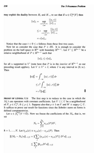
![Estimates in the Sobolev -1/2 Norm 231
= L II A;I/2 (pbj,k Dju ) 110
j
= L Ilpbj ,k A;I/2Dju + [A;I/2,pbj,k]Djullo
j
+ L II[A;1/2,pbj,k]Djullo'
j
Note that if W is small enough then sUPw Ipbj,kl < E since Ibj,k(P)1 == O. Now
the commutator in the second sum is of tangential order - 3/2. Thus the last
line is
;S E L
j
II, Dju lll-I/2 +L
j
III
Dju lll-3/2
where (shrinking V if necessary) we have applied Lemma 7.7.6. As a result,
III N k u lll-I/2 ~ III M k u lll-I/2 + III(Mk - Nk)ulll-I/2
;S IIIMk u lll-I/2 + E L III Dju lll-I/2. (7.7.5.2)
j
If we can prove the constant coefficient case of our inequality then we would
have
N
"'"2'" N ulil-I/2 + Jan lui·
LrIIIDJulll-l/2 ;S ~ 2 r III k 2
Coupling this with (7.7.5.2) would yield
The full result then follows.](https://image.slidesharecdn.com/partialdifferentialequationsandcomplexanalysis-121120212851-phpapp02/85/Partial-differential-equations-and-complex-analysis-242-320.jpg)
![232 The a-Neumann Problem
So we have reduced matters to the case of the Mk's having constant coeffi-
cients. Assume for the moment that u Ian == O. Then we can extend u to be
zero outside O. The extended function will be continuous on all of space. We
may suppose that V is a special boundary chart. Notice that, on V, the Di u
are continuous and Dr U has only a jump discontinuity. Therefore all of these
first derivative functions are square integrable.
Write ~ == (T, () with T E ~2n-l ,( E ~. We use the symbol condition on the
Mk's to see that
N
L IIIMkulll~1/2
k=l
( Plancherel in)
IaSl=var. t;
N
11(1 + IrI 2)-1/4
[2n-l
f; aj,k(P)rj
+ a2n,k(p)(] u(~) 116
N
L l2n (1 + IrI 2)-1/2Ia(Nk, ~)12Iu(~)12 d~
k=l
> l2n (1 + IrI2)-1/21~12Iu(~)12 d~
> l2n (1 + IrI 2)-1/2 ( ~ IDjUI2) (~) d~
L IIIDjulll~1/2 .
j
Therefore
N 2n
L IIIMkulll~1/2 ~ L IIIDjulll~1/2
k=l j=l
in the constant coefficient case provided that u vanishes on ao.
Next suppose that u mayor may not vanish at the boundary. Let
w(r,r) == exp [(1 + Ir I2)1/2 r ] u(r,O).
This is a regular extension of u(T, 0) to (T, r), r ~ O. By the Fourier inversion
theorem we have
w(t,O) == u(t, 0).](https://image.slidesharecdn.com/partialdifferentialequationsandcomplexanalysis-121120212851-phpapp02/85/Partial-differential-equations-and-complex-analysis-243-320.jpg)
![Estimates in the Sobolev -112 Norm 233
Set v == u - w. Then v vanishes on the boundary so that the previous result
applies to v. We then have
Therefore
2n 2n
L IIIDjulll~I/2 ;S L IIIDjvlll~I/2 + IIIDjwlll~I/2
j=1 j=1
N 2n
;S L IIIMkvlll~I/2 + L IIIDjwlll~I/2
k=1 j=1
N 2n
;S L [IIIMkUIII~I/2 + IIIMkWIII~I/2] + L IIIDjwlll~I/2
k=1 j=1
since the M k 's are linear combinations of the Dj,s. Observe that we are finished
if we can show that
j ==1, ... ,2n.
First suppose that j E {I, ... , 2n - I}. Then
IIIDjwlll~'/2 = 1.2n-l £°00 (1 + Ir I2)-1/2I rjI2exp [2(1 + Ir I2)1/2 r]
2
x 111,(r, 0) 1 dr dr
;S 1.2n-l £°00 (1 + IrI 2)-'/2(1 + Ir1 2)exp [2(1 + Ir I2)1/2 r]
2
x lu(r,0)1 drdr
= r lu(r,0)12(~exP[2(1+ITI2)1/2r]IO) dT
JJR.2n-l 2 -00
== -2
1
r
JJR.2n-l
lu( r, 0) 2 dr 1
=
1 r
2: Jan lui
2
da.](https://image.slidesharecdn.com/partialdifferentialequationsandcomplexanalysis-121120212851-phpapp02/85/Partial-differential-equations-and-complex-analysis-244-320.jpg)
![234 The a-Neumann Problem
If instead j == 2n, so that Dj is the usual normal derivative, then
Since the derivative does not affect the variables in which we take the Fourier
transform, the two operations commute. Hence
Therefore
mDrwlll~'/2 = l,n-l 1 0
00 (1 + Ir I2)-1/2(1 + Ir1 2) exp [2(1 + Ir I2)1/2 r ]
2
x lu(r,O)1 drdr
= l,n-l 1 0
00 (1 + IrI 2)1/2 exp [2(1 + I r I 2 )1/2 r ]lu(r,O)1 2 drdr
1
== -2 { lu(r,O)1 2 dr
JJR.2n-l
= ~ ~n lul
2
deY.
This concludes the second case and the proof. I
7.8 Conclusion of the Proof of the Main Estimate
Now we pass from the Sobolev -1/2 norm to higher order norms.
LEMMA 7.8.1
Suppose that the basic estimate E (¢)2 ;S Q (¢, ¢), ¢ E 1J p ,q, holds on a special
boundary chart V. Let {Pk} be a sequence of cutoff functions in A~'o (V n 0)
such that
Pk =1 on SUPPPk+l.
Then for each k > 0 we have an a priori estimate](https://image.slidesharecdn.com/partialdifferentialequationsandcomplexanalysis-121120212851-phpapp02/85/Partial-differential-equations-and-complex-analysis-245-320.jpg)
![Conclusion of the Proof of the Main Estimate 235
PROOF We proceed by induction on k. For k == 1 we have
(basic est.)
~ Q(PI¢, PI¢)
(7~3) ReQ(¢,PI¢) + O(II¢1I6)
(Frie~chs) Re (F¢, pr¢) + O(II¢1I6)
~ IIF¢llo IIpr¢lIo + O(II¢1I6)
~ I F¢lIoll¢llo + O(II¢1I6)
~ IIF¢116 + O(II¢1I6)
~ IIF¢1I6
~ IIIPIF¢III~I/2 + II F ¢116'
In the last two lines but one we have used the fact that T == F- 1 is bounded
on £2. This is the first step of the induction.
Now take k > 1 and assume that we have proved the result for k - 1. Set
A == A~k-I)/2. Note that A commutes with Dj,j == 1, ... ,2n - 1, because A
is a convolution operator in the tangential variables. If j == 2n then it is even
easier to see that Dj commutes with A since A does not act in the r variable.
Thus
I I V Pk¢III(k-2)/2 == I I A (V Pk¢) 1II~1/2
== IIIVA(Pk¢)III~I/2
== IIIVA(PIPk¢)III~I/2' (7.8.1.1)
Observe that
[A, [Dj, PI]] PkPk-l¢ + [A, PI][Dj, Pk]Pk-l¢ + [A, PI]Pk Dj Pk-l¢
[A, [Dj, pd] PkPk-l¢ + [A, pdDj PkPk-l¢
(Jacobiidentity) _ [PI, [A,Dj]J PkPk-l¢ - [Dj, [PI,A]J PkPk-l¢
+ [A, pdDj PkPk-l¢
(A, Dj S9mmute) 0 Dj [A] A.
- - - PI, PkPk-11.f/](https://image.slidesharecdn.com/partialdifferentialequationsandcomplexanalysis-121120212851-phpapp02/85/Partial-differential-equations-and-complex-analysis-246-320.jpg)
![236 The a-Neumann Problem
As a result,
Dj APIPk¢ == Dj PIApk¢ + Dj[A, pdPk¢
== Dj PIApk¢ + [A, [Dj, pd] PkPk-l¢ + [A, pd [Dj, Pk]Pk-1 ¢
+ [A, pdPk Dj Pk-l¢.
Therefore, using (7.8.1.1),
I I V Pk¢lII(k-2)/2 == IIIVApIPk¢III~I/2
;S IIIVPIApk¢III~I/2 + L I I [A, [Dj,pd] PkPk-I¢II'~1/2
j
+ L I I [A, pd[Dj, Pk]Pk-I¢III~I/2
j
+ L I I [A, pdPk Dj Pk-I¢III~I/2
j
;S IIIV PIApk¢III~I/2 + IIIPk-I¢III~I/2+(k-3)/2
IIIPk-1 ¢III~ 1/2+(k-3)/2 + IIIVPk-l ¢III~ 1/2+(k-3)/2
;S IIIVPIApk¢III~I/2 + I I V Pk-I¢III(k-3)/2' (7.8.1.2)
Consider the term IIIVPIApk¢III~I/2 on the right-hand side. Set
-
PIApk == PI A(k-I)/2 Pk == A .
t
-
Then
IIIVApk-I¢I"~1/2
<
rv Q(Apk-I¢, Apk-l¢)
Re Q(Pk-1 ¢, A' APk-1 ¢)
+ (1 (IIIV' Pk-l ¢IIIZk-3)/2)
(Pk-I~=A') Re Q( ¢, A' APk-l ¢) + (1 (IIIV' Pk-l ¢IIIZk-3)/2)
Re (F¢, A' Apk-l¢) + O(IIIV Pk-I¢III(k-3)/2
Re (AF¢, APk-1 ¢) + (1 (IIIV' Pk-l ¢IIIZk-3)/2)](https://image.slidesharecdn.com/partialdifferentialequationsandcomplexanalysis-121120212851-phpapp02/85/Partial-differential-equations-and-complex-analysis-247-320.jpg)
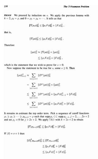
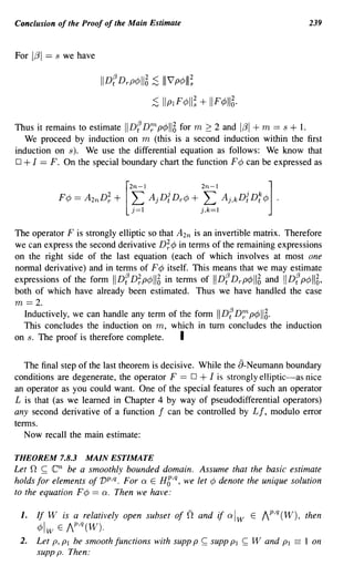
![240 The a-Neumann Problem
(a) If W n an == 0 then Vs 2: 0 there is a constant Cs > 0 (depending
on P, PI but independent of a) such that
(7.8.3.2a)
(b) If W n an =I- 0 then Vs 2: 0 there exists a constant Cs 2: 0 such that
(7 .8.3.2b)
REMARK In the theorem that we just proved, we established the a priori esti-
mate
That is, we know that this inequality holds for a testing function ¢. In the Main
Estimate we are now addressing the problem of existence: given a v E H6,q we
want to know that there exists a ¢ which is smooth and satisfies (7.8.3.2a) and
(7.8.3.2b). We do know that the ¢ given by Friedrichs is in L 2 , but nothing
further. It is in these arguments that the elliptic regularization technique comes
to the rescue. In the original papers [KOHl] Kohn had to use delicate functional
analysis techniques to address the existence issue. I
PROOF OF THE MAIN ESTIMATE Let a E H6,q. Let ¢ E vp,q be the unique
solution to the equation F ¢ == a. This will of course be the ¢ that we seek,
but we must see that it is smooth. Observe that this assertion, namely part (I)
of the theorem, follows from part (2).
Let U be a subregion of en.
Assume that
p,q -
a Iunn E I (UnO).
We need to see that
4>lunn E Ip,q (U n D).
The easy case is if U n an == 0. For then ¢ Iu E Ip,q (U) by the interior
elliptic regularity for F == 0 + I. This gives us the estimate (7 .8.3.2a) as well.
Refer to Chapter 4 for details.
More interesting is the case U n an
=I- 0. Then the last theorem tells us that
provided that we know in advance that ¢ is smooth on uno. Again we
emphasize the importance of this subtlety: we know that ¢ exists; we also know
that if ¢ is known to be smooth on unothen it satisfies the desired regularity
estimates. We need to pass from this a priori infonnation to a general regularity
result. To this task we now tum.](https://image.slidesharecdn.com/partialdifferentialequationsandcomplexanalysis-121120212851-phpapp02/85/Partial-differential-equations-and-complex-analysis-251-320.jpg)
![244 The a-Neumann Problem
COROLLARY 7.9.3
If F¢ == a and a E Hf,q then ¢ E H~:1 and 11¢lls+l ;S Iiali s.
PROOF Immediate. I
COROLLARY 7.9.4
The operator F- 1 is a compact operator on Hf,q.
PROOF By the corollary we know that F- 1 is bounded from Hf,q to H~~1 so
we apply Rellich's lemma to obtain the result. I
COROLLARY 7.9.5
The operator F has discrete spectrum with no finite limit point and each eigen-
value occurs with finite multiplicity.
PROOF By the theory of compact operators (see, for instance, [WID]), we know
that F- 1 has countable, compact spectrum with 0 as its only possible limit point.
Also each eigenvalue has finite multiplicity. Since A is an eigenvalue for F if
and only if A-1 is an eigenvalue for F- I we have proved the corollary. I
PROPOSITION 7.9.6
Let U, P, PI, a, and k be as in Proposition 7.9.1. Suppose that PI a E Hf,q for
some integer s > o. If ¢ satisfies (F - A)¢ == a for some constant A then
p¢ E H~:k(n).
PROOF Consider the case k == 1. Set a' == a + A¢. Then ¢ satisfies the
equation F¢ == a'. Now a' E H6,q so that PI¢ E Hi,q by Proposition 7.9.1.
Let {Pk}k=2 be a sequence of smooth functions with Ps == P and Pj = 1 on
supp Pj + 1. Inductively we may reason that
The result follows.
The case k == 2 is similar. I
COROLLARY 7.9.7
The operator F - AI is hypoelliptic.
PROOF Immediate from the proposition and Sobolev's theorem. I](https://image.slidesharecdn.com/partialdifferentialequationsandcomplexanalysis-121120212851-phpapp02/85/Partial-differential-equations-and-complex-analysis-255-320.jpg)
![246 The a-Neumann Problem
PROOF First of all we need to show that range (D F) is closed. Set HP,q ==
kernel (0 F ). Then HP,q is the eigenspace corresponding to the eigenvalue O.
The orthogonal complement of HP,q is E9!AI>o VA, where VA is the eigenspace
corresponding to the eigenvalue A. Then 0 F is bounded away from 0 on
°
(HP,q) 1.. and it is one-to-one on this space. Thus F restricted to the closure
°
of the range of F has a continuous inverse which we call L.
Let DFx n --+ y. Then LDFx n --+ Ly, that is, X n ~ Ly and DF(Ly) == y.
Thus y E range 0 F and range 0 F is closed. Since range 0 F == (HP,q) 1.., the
first equality follows.
a
For the second equality, notice that 2 == 0 hence range -l range a Also a*.
a* == {) Idom [j* and the second equality follows as well. I
COROLLARY 7.9.11
- - 1
The range of 8 on dom (8) n H6,q- is closed.
PROOF a
Since range -l kernel and (a*) a* ({)a dom (F) EB 1tp,q) == 0, we may
conclude that range ==a a{)
dom (F). I
a
We are engaged in setting up a Hodge theory for the operator. For analogous
material in the classical setting of the exterior differential operator d we refer
the reader to [CON].
Now we define the hannonic projector H to be the orthogonal projection
from Hb,q onto HP,q. We use that operator in tum to define the a-Neumann
operator.
DEFINITION 7.9.12 The Neumann operator N : H6,q ~ dom (F) is defined
by
Na == 0 if a E rtp,q
Na == ¢ if a E range 0 F and ¢ is the unique
solution of °F¢ == a with ¢ -l HP,q.
Then we extend N to all of H6,q by linearity.
Notice that N a is the unique solution ¢ to the equations
H¢ == 0
DF¢==a-Ha.
Finally, we obtain the solution to the a-Neumann problem:](https://image.slidesharecdn.com/partialdifferentialequationsandcomplexanalysis-121120212851-phpapp02/85/Partial-differential-equations-and-complex-analysis-257-320.jpg)
![248 The a-Neumann Problem
Next we want to solve the inhomogeneous Cauchy-Riemann equation a¢ ==
a. Notice that there is no hope to solve this equation unless a ..1 kernel (a*) or
equivalently all'== 0 and H a == O.
THEOREM 7.9.14
Suppose that q 2 1, a E HC,q,
1
all'
== 0, and H a == O. Then there exists a
- - -
unique ¢ E HC,q- such that ¢..l kernel (B) and B¢ == a. Ita E AP,q(O) then
¢ E AP,q-l (0) and
PROOF By the conditions on a we have that a == a{) N a. Thus we take
¢ == () N a and ¢ ...L kernel (a) implies uniqueness. By part (4) of the last
theorem, we know that Na E AP,q if a E AP,q. Hence ¢ E AP,q-l and
1I¢lIs == II{)Nails
;S IINall s+l
~ Iiall s . I
It is in fact the case that, on a domain in Euclidean space, the harmonic space
HP,q is zero dimensional. Thus the condition H a == 0 is vacuous. There is
no known elementary way to see this assertion. It follows from the Kodaira
vanishing theorem (see [WEL]), or from solving the a-Neumann problem with
certain weights. A third way to see the assertion appears in [FOK]. We shall
say no more about it here.
In fact, it is possible to prove a stronger result than 7.9.14: if a has H S
coefficients, then ¢ has H s+ 1/2 coefficients. This gain of order 1/2 is sharp for
o strongly pseudoconvex. We refer the reader to [FOK, p. 53] for details.
Appendix to Section 7.8: Uniform estimates for F 8 and ¢8
Refer to Section 7.8-especially the proof of the Main Estimate-for terminol-
ogy. The purpose of this appendix is to prove that the estimate
(7.A.l)
holds with a constant that is independent of 8. We begin as follows:
PROPOSITION 7.A.2 We have
where the constant in 0 is independent of b.](https://image.slidesharecdn.com/partialdifferentialequationsandcomplexanalysis-121120212851-phpapp02/85/Partial-differential-equations-and-complex-analysis-259-320.jpg)
![Appendix to Section 7.8 249
PROOF The proof of 7.7.2 goes through, with [) replaced by any first-order
differential operator D with constant coefficients, without any change. Thus
(DA¢, DA¢) - Re (D¢, DA' A¢) == O(IIIV¢III~_l)'
Then
Q8(A¢, A¢) - Re Q8(¢, A' A¢) == Q(A¢, A¢) + 8 L(Dj A¢, Dj A¢)
j
- Re [Q(I/>, A'AI/» + 8 L(Dj 1/>, Dj A'AI/»]
J
== Q(A¢,A¢) -ReQ(¢,A'A¢)
+ 8 L [(Dj AI/>, Dj AI/» - (Dj 1/>, Dj A'AI/»]
J
== (1 + 8)0 (1IIV¢III~-l)
== 0 (IIIV ¢III~-I) ,
where the constant in 0 is independent of 8. I
We need one more preliminary result:
PROPOSITION 7.A.3 Let hypotheses be as in 7.8.1 with ¢ E v~,q. Then
(7 .A.3.t)
where the constants are independent of 8.
PROOF We follow the proof of 7.8.1 closely, checking that all constants that
arise are independent of 8. We induct on k. First let k == 1. Then
(7.7.4)
<
(basic estimate) 8 8
:S Q(Pl¢ , PI¢ )
< Q8 (PI ¢8, PI ¢8)
(7.~.2)
ReQ8(¢8,pf¢6) + 0 (11¢8116)
(Frie~chs)
Re (F 8¢8,pf¢8) + 0 (11¢8116)
IIF 8¢c5 lloll¢ c5 llo + 0 (11¢8116) .
Notice that Tb = (pc5)-I is bounded on £2 unifonnly in b. Indeed, by the](https://image.slidesharecdn.com/partialdifferentialequationsandcomplexanalysis-121120212851-phpapp02/85/Partial-differential-equations-and-complex-analysis-260-320.jpg)
![8
Applications of the 8-Neumann Problem
8.1 An Application to the Bergman Projection
In recent years the Bergman projection P : L 2 (0-) ---+ A 2 (0-) has been an
object of intense study. The reason for this interest is primarily that Bell and
Ligocka [BEL], [BE 1], [BE2] have demonstrated that the boundary behavior of
biholomorphic mappings of domains may be studied by means of the regularity
theory of this projection mapping. Of central importance in these considerations
is the following:
DEFINITION 8.1.1 CONDITION R Let 0- ~ en
be a smoothly bounded do-
main. We say that 0- satisfies Condition R if P maps Coo ((2) to Coo ((2).
A representative theorem in the subject is the following:
THEOREM 8.1.2 BELL
Let 0- 1,0- 2 be smooth, pseudoconvex domains in en.
Let <I> : 0- 1 ---+ 0- 2 be a
biholomorphic mapping. If at least one of the two domains satisfies Condition
R then <I> extends to a Coo diffeomorphism of 0- 1 to 0- 2 .
There are roughly two known methods to establish Condition R for a domain.
One is to use symmetries, as in [BAR] and [BEB]. The more powerful method
is to exploit the a-Neumann problem. That is the technique we treat here. Let
us begin with some general discussion.
Let 0- c c en be a fixed domain on which the equation au == Q is always
solvable when Q is a a-closed (0,1 )-form (e.g., a domain of holomorphy-in
other words, a pseudoconvex domain). Let P : L 2(0-) ---+ A2(0-) be the Bergman
projection. If u is any solution to au == Q then W == Wet == U - Pu is the unique
solution that is orthogonal to holomorphic functions. Thus W is well defined,
independent of the choice of u. Define the mapping](https://image.slidesharecdn.com/partialdifferentialequationsandcomplexanalysis-121120212851-phpapp02/85/Partial-differential-equations-and-complex-analysis-263-320.jpg)
![An Application to the Bergman Projection 253
Then, for f E L 2 (n) it holds that
Pf == f - T([)f)· (8.1.3)
To see this, first notice that [)[f - T( [) f)] == [) f - [) f == 0, where all derivatives
are interpreted in the weak sense. Thus f - T( [) f) is holomorphic. Also f -
[f - T( [) f)] is orthogonal to holomorphic functions by design. This establishes
the identity (8.1.3). But we have a more useful way of expressing T: namely
T == [)* N. Thus we have derived the following important result:
P == I - [)* N8. (8.1.4)
Now suppose that our domain is strongly pseudoconvex. Then we know that
N maps HS to Hs+ 1 for every s. Recall that [) and [)* are first-order differential
operators. Then a trivial calculation with (8.1.4) shows that
for every s. By the Sobolev imbedding theorem, a strongly pseudoconvex
domain therefore satisfies Condition R. Thus, thanks to the program of Bell
and Ligocka (see [BEL], [KR1]), we know that biholomorphic mappings of
strongly pseudoconvex domains extend to be diffeomorphisms of their closures.
It is often convenient, and certainly aesthetically more pleasing, to be able to
prove that P : H S -+ H s. This is known to be true on strongly pseudoconvex
domains. We now describe the proof, due to J. J. Kohn [KOH3], of this assertion.
THEOREM 8.1.5
Let n be a smoothly bounded strongly pseudoconvex domain in en. Then for
each s E IR. there is a constant C == C (s) such that
(8.1.5.1)
REMARK In fact, the specific property of a strongly pseudoconvex domain that
will be used is the following: For every E > 0 there is a C (E) > 0 so that the
inequality
(8.1.5.2)
o1 - -
for all 1; E 1) == / ' n dom {) n dom {)*. We leave it as an exercise for
the reader to check that property (8.1.5.2) is equivalent to the norm Q being
compact in the following sense: if {1;j} is bounded in the Q nonn then it has
a convergent subsequence in the £2 nonn.](https://image.slidesharecdn.com/partialdifferentialequationsandcomplexanalysis-121120212851-phpapp02/85/Partial-differential-equations-and-complex-analysis-264-320.jpg)
![254 Applications of the 8-Neumann Problem
The theorem that we are about to prove is in fact true on any smoothly
bounded domain with the property (8.1.5.2). Property (8.1.5.2) is known to
hold for a large class of domains, including domains of finite type (see [CAT1],
[CAT2], [DAN1], [DAN2], [DAN3], [KR1]) and, in particular, domains with
real analytic boundary ([DF]). I
PROOF OF THE THEOREM We have already observed that the Bergman projec-
tion of a strongly pseudoconvex domain maps functions in Coo (n) to functions
in Coo (n). Thus it suffices to prove our estimate (8.1.5.1) for j E Coo (n).
Let r be a smooth defining function for n. Let ( E an and let U ~ en
be a neighborhood of (. We may select a smooth function w on U such that
n ar
w == w· satisfies Iwnl == 1 on U. We select wl, ... ,w n - l on U such that
wI, ... , w n forms an orthononnal basis of the (1, O)-forms on U. Thus any
n
¢ E V o,I can be expressed, on n U, as a linear combination
Of course, ¢ E VO,1 if and only if ¢n == 0 on an.
Let Al be the tangential Bessel potential of order s, as defined in Section
7.5. If 7] is any real-valued cutoff function supported in U then, whenever
¢ E VO,1 we have 7]AI(7]¢) E VO,1 as well. The identity Q(NQ,~) == (Q,~),
with Q == 8 j and 1/J == 7]3 A2s 7]N 8 j, yields that
(8.1.5.3)
Now we apply the compactness inequality (8.1.5.2) with ¢ == 7]AI(7]N8j) to
obtain
117]A:(7]N8j)II 2 :::; EQ(7]A:(7]N8j), 7]A:(7]NfJj)) + C(E)II7]A:(7]N8j)II~1
:::; EQ(N8j, 7]3 A;s7]NfJj) + ECII NfJj II; + C'(E)IIN8jll;_1.
Of course in the last estimate we have done two things: First, we have moved 7]
and Af across the inner product Q at the expense of creating certain acceptable
error terms (which are controlled by the term ECIINfJjll;). Second, we have
used the fact that IIAI 9116 :::; IIgll; by definition. Now, using (8.1.5.3), we see
that
117]A:(7]NfJj)II 2 :::; E(j, fJ*7]3 A;s7]N8j) + ECIINfJjll;
+C'(E)IINfJjll;_I· (8.1.5.4)
Now we may cover n
with boundary neighborhoods U as above plus an
interior patch on which our problem is strongly elliptic. We obtain an estimate
like (8.1.5.4) on each of these patches. We may sum the estimates, using
(as we did in the solution of the 8- Neumann problem) the fact that is an](https://image.slidesharecdn.com/partialdifferentialequationsandcomplexanalysis-121120212851-phpapp02/85/Partial-differential-equations-and-complex-analysis-265-320.jpg)
![An Application to the Bergman Projection 255
noncharacteristic for Q, to obtain
Applying this inequality, with s replaced by s - 1, to the last term on the right,
and then repeating, we may finally derive that
(8.1.5.5)
We know that 88* N af == af. As a result,
II 1JA:1]a* N8fll 2 == (N8f, 1]3 A;s1]aa* N8f) + 0 (liNafils II1]A:1]8* N8fll)
== (N8f, 1]3A;s1]8 f) + 0 (liN 8fils II1]A:1]8* N8fll)
= o( (11 N8/11s + III lis) IlryA:ry8*N8/11 ).
Summing as before, we obtain the estimate
IIa* Naflls ~ c(IINaflls + Ilflls).
Putting (8.1.5.5) into this last estimate gives
If we choose E > 0 small enough, then we may absorb the first term on the
right into the left-hand side and obtain
lIa* Naflls ~ C· (IIflls + II N8 fllo) . (8.1.5.6)
But the operator a* is closed since the adjoint of a densely defined operator
is always closed. It follows from the open mapping principle that
On the other hand, a*Na is projection onto the orthogonal complement of
A 2 (n). Thus it is bounded in £2 and we see that
IINafll ~ cllfllo.
Putting this information into (8.1.5.6) gives](https://image.slidesharecdn.com/partialdifferentialequationsandcomplexanalysis-121120212851-phpapp02/85/Partial-differential-equations-and-complex-analysis-266-320.jpg)
![256 Applications of the a·Neumann Problem
If we recall that P == I - [)* N [) then we may finally conclude that
IIPIlIs :::; CIIIlIs.
That concludes the proof. I
8.2 Smoothness to the Boundary of Biholomorphic Mappings
In this section we shall use the fact that Condition R holds on any strongly pseu-
doconvex domain (Theorem 8.1.5) to prove the following theorem of Fefferman
(this generalizes the one-variable result from Section 1.5):
THEOREM 8.2.1
Let n ~ en be a strongly pseudoconvex domain with smooth boundary and <I> :
n n a biholomorphic mapping.
---+ Then <I> extends uniquely to a diffeomorphism
ojn to n.
As already indicated, the proof given here is that of Bell [BE2] and Bell and
Ligocka [BEL]. It will be particularly convenient for us to use the following form
of Condition R that we proved in the last section: If P is the Bergman projection
on the strongly pseudoconvex domain nand s E IR. then P : H s ---+ H s.
Observe that the "uniqueness" portion of Theorem 8.2.1 is virtually a tautol-
ogy and we leave its consideration to the reader. We build now a sequence of
lemmas leading to the more interesting "smoothness" assertion of Fefferman's
theorem. We begin with some notation.
If nee en
is any smoothly bounded domain and if j E N, we let
11,1 (n) == Hj (n) n {holomorphic functions on n},
H oo (n) == n00
j=l
Hj (n) == Coo (0.) n {holomorphic functions on n}.
Here Hj is the standard Sobolev space on a domain. Let Hg (n) be the Hj clo-
sure of Cgo (n). (Exercise: if j is sufficiently large, then the Sobolev imbedding
theorem implies trivially that H6 (n) is a proper subset of Hj (n).)
Let us say that u, v E Coo (0.) agree up to order k on an if
(:z) a (:z)~ (u - V)I == 0 Va,f3 with lal + 1f31 :::; k.
an](https://image.slidesharecdn.com/partialdifferentialequationsandcomplexanalysis-121120212851-phpapp02/85/Partial-differential-equations-and-complex-analysis-267-320.jpg)
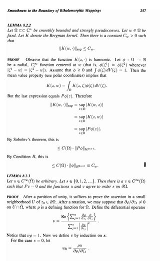
![258 Applications of the a·Neumann Problem
Define
a
Vo == a(1 Wo
== u + O(p).
Then u and Vo agree to order 0 on an. Also
PVo(z) = J K(z, () 8~1 wo(() dV(().
This equals, by integration by parts,
-J8~1 K(z, ()wo(() dV(().
Notice that the integration by parts is valid by Lemma 8.2.2 and because
Wo Ian == O. Also, the integrand in this last line is zero because K (z, .) is
conjugate holomorphic. Thus Pvo == 0 as desired.
Suppose inductively that W s -l == W s -2 + Os_Ips and V s -l == (a/az 1 )(W s -l)
have been constructed. We show that there is a W s of the fonn
such that V s == (a/az 1 )(w s ) agrees to order s with u on an. By the inductive
hypothesis,
a
Vs == -a W s
ZI
- aW - + - [0 s·p s+l]
_ - s -l a
aZ I aZ I
= Vs-I + Ps [(
s
ap
+ 1) OS 8Z 1 + p. ao s ]
8z]
agrees to order s - 1 with u on an so long as Os is smooth. So we need
to examine D(u - vs), where D is an s-order differential operator. But if D
involves a tangential derivative Do, then write D == Do . D 1• It follows that
D(u - vs) == Do(a), where a vanishes on an so that Doa == 0 on an. So we
need only check D == v S •
We have seen that Os must be chosen so that
on an.](https://image.slidesharecdn.com/partialdifferentialequationsandcomplexanalysis-121120212851-phpapp02/85/Partial-differential-equations-and-complex-analysis-269-320.jpg)
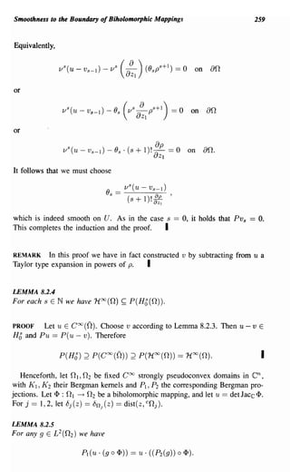
![260 Applications of the a-Neumann Problem
PROOF Notice that u· (g 0 4» E £2(0}) by change of variables (see Lemma
6.2.9). Therefore, by 6.2.8,
P1(u· (g 0 4»)(z) == 1
01
K}(z,()u(()g(4>(()) dV(()
== 1
0 1
u(z)K2 (4>(z), 4>(())u(()u(()g(4>(()) dV(().
Change of variable now yields
PI (U· (g 0 4»)(Z) == u(z) 1O2
K 2(4)(z), ~)g(~) dV(~)
== U(Z) . [( P2(g)) 0 4>] (Z). I
Exercise: Let nee en be a smoothly bounded domain. Let j E N. There is
an N == N(j) so large that 9 E He' implies that 9 vanishes to order j on an.
LEMMA 8.2.6
Let ~ : n1 ---+ n2 be a CJ diffeomorphism that satisfies
(8.2.6.1)
for all multiindices a with Ia I :s; j E Nand
(8.2.6.2)
Suppose also that
82 ( ~ ( z)) :s; C 81 ( Z ) . ( 8.2.6.3 )
Then there is a number J == J(j) such that, whenever 9 E HZ+ J
(n 2 ), then
go~ E HZ(n 1 ).
PROOF The subscript 0 causes no trouble by the definition of HZ. Therefore
it suffices to prove an estimate of the form
By the chain rule and Leibniz's rule, if a is a multiindex of modulus not ex-
ceeding j, then
where 1,81 :s; lal,2: 11'il :s; lal, and the number of tenns in the sum depends
only on a (a classical formula of Faa de Bruno--see [ROM]-actually gives](https://image.slidesharecdn.com/partialdifferentialequationsandcomplexanalysis-121120212851-phpapp02/85/Partial-differential-equations-and-complex-analysis-271-320.jpg)
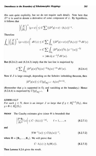
![262 Applications of the a.Neumann Problem
To prove (8.2.6.3), let p be a smooth, strictly plurisubharmonic defining func-
n
tion for l . Then p 0 <1>-1 is a smooth plurisubharmonic function on nz. Since
p vanishes on an I and since <1> -I is p~oper, we conclude that p 0 <I> -I extends
continuously to (2z. If P E an z and vp is the unit outward normal to an z at P,
then Hopf's lemma (see our treatment in Section 1.5 Of, for a different point of
view, consult [KRAl, Chapter 1]) implies that the (lower) one-sided derivative
(a / avp ) (p 0 <1>-1) satisfies
8
(p 0 <I> -I (P)) ~ c.
avp
So, fOf W == P - EVp, E >0 small, it holds that
These estimates are uniform in P E an z. Using the comparability of Ipl and 81
yields
Setting z == q, -1 ( w) now gives
which is (8.2.6.3). I
LEMMA 8.2.8
The function u is in COO((2I).
PROOF It suffices to show that u E Hi (n l ), every j. So fix j. According
to (8.2.7.1), lu(z)1 ::; C8 1 (z)-Zn. Then, by Lemma 8.2.7 and the exercise for
J
the reader preceding 8.2.6, there is a J so large that 9 E HZ+ (n z) implies
u . (g 0 <1» E Hi (n l ). Choose, by Lemma 8.2.4, agE Hf:+J (n z) such that
Pzg == 1. Then Lemma 8.2.5 yields
PI (u . (g 0 <1») == u.
By Condition R, it follows that u E Hi (n l ). I
LEMMA 8.2.9
The function u is bounded from 0 on (21.
PROOF By symmetry, we may apply Lemma 8.2.8 to <1>-1 and det Jc (<1>-1)
== l/u. We conclude that l/u E COO(Oz). Thus u is nonvanishing on O. I](https://image.slidesharecdn.com/partialdifferentialequationsandcomplexanalysis-121120212851-phpapp02/85/Partial-differential-equations-and-complex-analysis-273-320.jpg)
![Other Applications of [) Techniques 263
PROOF OF FEFFERMAN'S THEOREM (THEOREM 8.2.1) Use the notation of the
proof of Lemma 8.2.8. Choose gl, ... ,gn E Hg O+J
(n 2 ) such that P2gi (w) == Wi
(here Wi is the i th coordinate function). Then Lemmas 8.2.5 and 8.2.7 yield that
U· <Pi E Hj(n 1 ), i == 1, ... , n. By Lemma 8.2.9, <Pi E Hj(n 1 ), i == 1, ... , n.
By symmetry, <p- 1 E Hj (n 2 ). Since j is arbitrary, the Sobolev imbedding theo-
rem finishes the proof. I
8.3 Other Applications of aTechniques
The unifying theme of this book has been the theory of holomorphic mappings.
We have seen that regularity for the classical Dirichlet problem for the Laplacian
provided the key to understanding boundary regularity of conformal mappings in
the complex plane. Likewise, boundary regularity for the a-Neumann problem
has provided the key for determining the boundary behavior of biholomorphic
mappings of several complex variables.
Since we have gone to so much trouble to derive estimates for the a-Neumann
problem, it seems appropriate at this time to depart from our principal theme
a
and discuss some other applications of our results on the problem.
A point that hampered the theory of the Bergman kernel for years was that
of boundary regularity. On the ball, for example, one sees that the Bergman
kernel blows up if z, ( E B approach the same boundary point. But on B x B
(diagonal) the Bergman kernel is smooth. One might hope that a similar result
is true on, say, strongly pseudoconvex domains (the question is open for general
smoothly bounded domains). Heartening partial results on this problem were
made by Diederich in [DIE]. However, Kerzman [KER2] realized that the result
follows easily from a-Neumann considerations. Here is a part of what Kerzman
proved (this result is implicit in one of the lemmas from the last section):
PROPOSITION 8.3.1
n
Let ~ en be smoothly bounded and strongly pseudoconvex. Fix zEn. Then
K(z, . ) is in C OO ((2).
PROOF Let ¢ E C~ (en) be a nonnegative radial function of total mass one
and with support in the unit ball. Define ¢E(() == E- 2n ¢((/E). Choose E to be
a positive number less than the Euclidean distance of z to the boundary of n.
Because K is harmonic in the first variable we have, by the mean value
property, that
K(w,z) = J K(w,l;)¢{(z-l;)dV(l;).
But this last (a function of w) also equals the Bergman projection of ¢E (z - .).
Since ¢€ (z - .) E CCXJ (n) and n satisfies condition R, we may conclude that](https://image.slidesharecdn.com/partialdifferentialequationsandcomplexanalysis-121120212851-phpapp02/85/Partial-differential-equations-and-complex-analysis-274-320.jpg)
![264 Applications of the a·Neumann Problem
K(·, z) E COO(n). But the Bergman kernel is conjugate symmetric in its
variables; that finishes the proof. I
A fundamental problem in the complex function theory of both one and several
complex variables is to take a local construction of a holomorphic function and
tum it into a global construction. In one complex variable we have the theorems
of Weierstrass and Mittag-Leffler, Cauchy formulas, conformal mapping, and
many other devices for achieving this end. In several complex variables, the
a-Neumann problem is certainly one of the most important tools (along with
sheaf theory and integral fonnulas) for this type of problem.
n
To illustrate this circle of ideas, let be a smoothly bounded, strongly pseu-
doconvex and smooth. Then for any defining function p and P E 8n we know
that the Levi form
is positive definite on all W == (WI, ..• , wn ) satisfying
n 8p
'L oz. (P)Wj = O.
j=I J
(8.3.2)
This is the definition of strong pseudoconvexity. However it is an elementary
exercise in calculus to see that if A > 0 is large enough then the new defining
function
exp(Ap(z)) - 1
PA ()
Z == A
satisfies
(8.3.3)
for all wEen and some C > O. Details of this construction may be found in
[KRAl, Chapter 3].
Now with such a function PA in hand we define the Levi polynomial
Lp(z) ==
n
'L 8PA 1
-(P)(z· - p.) + - 'L
n 2
8 pA
--(P)(z· - P')(Zk - Pk).
8z. J J 2 8z .8z k J J
j=I J j,k=I J
The key technical result is this:
PROPOSITION 8.3.4
With n, P, Lp as above there is a 8 > 0 such that if Iz - PI < 8, z E 0, and
Lp(z) == 0 then z == P. See Figure 8.1.](https://image.slidesharecdn.com/partialdifferentialequationsandcomplexanalysis-121120212851-phpapp02/85/Partial-differential-equations-and-complex-analysis-275-320.jpg)
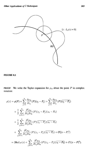
![Other Applications of [) Techniques 267
The Levi problem consists in showing that all pseudoconvex domains are
domains of holomorphy. This can be reduced, by relatively elementary means,
to proving the result for strongly pseudoconvex domains (see [KRl] for the
whole story). That in tum can be reduced to showing that each boundary point
P of a strongly pseudoconvex domain is essential: that is, there is a globally
n
defined holomorphic function G on that cannot be analytically continued past
P. In fact, that is what we have just proved.
It is not difficult to see that, on the ball with center P and radius 8, the real
part of L p is of one sign. Thus we may take a fractional root of this holomorphic
function. As a result, it may be arranged that 9 E L 2 (n). We leave it as an
exercise for the reader to provide details of the following assertion:
PROPOSITION 8.3.6
Let n be a smoothly bounded, strongly pseudoconvex domain. Let P E an.
Then there is an £2 holomorphic function on n (an element of A 2 (n)) that
cannot be analytically continued past P.
It is in fact possible to construct a function that is CCXJ on nand holomorphic
n
on that cannot be continued past any boundary point. This requires additional
techniques. See [HAS], [CAT3] for details of this result. Both the result of
the last proposition, and the result of this paragraph, are true on any smoothly
bounded (weakly) pseudoconvex domain.
We conclude this section with another illustration of [) techniques in an ap-
plication to the extension of holomorphic functions:
THEOREM 8.3.7
Let n ~ enbe smoothly bounded and strongly pseudoconvex. Let M == {z E
en : Zn n n M. If f is a holomorphic function on w then there
== O}. Let w ==
is a holomorphic function F on n such that Flw == f.
PROOF Let 7r : en
---+ M be given by 7r(ZI, •.. , zn) == (Zl, ... , Zn-l, 0).
Define w == n
n M and B == {z En:
7r(z) tJ. w}. Then Band ware disjoint
and relatively closed in n. Refer to Figure 8.2.
n
By the CCXJ Urysohn lemma ([HIR]) there is a Coo function ¢ on such that
¢ == 1 in a neighborhood of wand ¢ == 0 in a neighborhood of B. Now define
H(z) == ¢(z) . f(7r(z)).
Since the support of ¢ lies in the complement of B, the function H is well-
defined. And it extends f. But of course it is not holomorphic.
We endeavor to make H holomorphic by adding on a correction term: set
F(z) == H(z) + Zn . w(z). (8.3.7.1)](https://image.slidesharecdn.com/partialdifferentialequationsandcomplexanalysis-121120212851-phpapp02/85/Partial-differential-equations-and-complex-analysis-278-320.jpg)
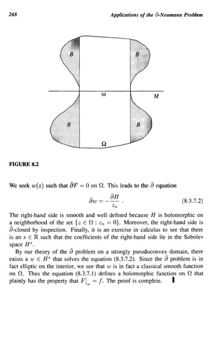
![9
The Local Solvability Issue and a Look Back
9.1 Some Remarks about Local Solvability
In the nineteenth century and the first half of the twentieth, it was generally be-
lieved that any partial differential equation with smooth coefficients and smooth
data would-at least locally-have smooth solutions. This belief was fueled, at
least in part, by the Cauchy-Kowalewski theorem, which says that this assertion,
with "smooth" replaced by "real analytic," is always true.
The Cauchy-Kowalewski theorem is the only general existence and regularity
theorem in the entire theory of partial differential equations (see [KRP] for a
treatment of this result). While fifty years ago it was thought to be typical, we
now realize that it represents the exception. Jacobowitz and Treves [JAT] have
shown that, in a reasonable sense, nonlocally solvable equations are generic.
H. Lewy presented the first nonlocally solvable partial differential equation
in [LEW2]. Lewy's equation is astonishingly simple. If the coordinates on }R3
are given by (x, y, t) ~ (x + iy, t) ~ (z, t), then the equation is
Lu == -
au + 7Z-
. au == f.
az at
Although it is not made explicit in that paper, Lewy's discovery grew naturally
out of analytic continuation considerations for holomorphic functions of two
complex variables. This assertion becomes clearer when the accompanying
paper [LEWl] is consulted.
The local solvability issue is also intimately connected with integrability for
systems of vector fields-specifically the vector fields arising as the real and
imaginary parts of holomorphic tangent vector fields to a strongly pseudoconvex
hypersurface. In particular, the Lewy equation is, in local coordinates, just the
tangential Cauchy-Riemann equations on a spherical cap; the issue of local
solvability for these equations is essentially equivalent (because the Levi form
is nondegenerate) to the issue of analytically continuing CR functions to the
(pseudo)convex side of the spherical cap.](https://image.slidesharecdn.com/partialdifferentialequationsandcomplexanalysis-121120212851-phpapp02/85/Partial-differential-equations-and-complex-analysis-280-320.jpg)
![270 The Local Solvability Issue and a Look Back
The local solvability question has received a great deal of attention since
Lewy's work. Hormander gave necessary conditions for the local solvability of
a linear partial differential operator (see [HOR1, Section 6.1]. Nirenberg and
Treves [NTR] gave necessary conditions for a partial differential operator of
principal type with smooth coefficients to be locally solvable. They also gave
sufficient conditions when the coefficients are real analytic. Beals and Fefferman
[BEF 1] showed that the Nirenberg-Treves condition is sufficient in general.
Our intention in this brief chapter is to exposit the basic ideas concerning local
solvability, with special emphasis on the connections with complex analysis.
Although much of this material can be presented in an entirely elementary
fashion (see Section 9.4), we position the subject last in the book so that we
may draw on the earlier chapters both for concepts and for motivation. We refer
the reader to [KOH2] and [NIR] for more on these matters; some of the material
presented here is drawn from those references.
9.2 The Szego Projection and Local Solvability
In order to be as explicit as possible, we shall work with the Siegel upper
half-space
with boundary
M == {z E ((:2 : Imz2 == I Z lI
2}.
It is worth noting explicitly that U is biholomorphic to the ball B: the mapping
<Pl(Z) == ~
1 + Zl
, 1 - Zl
<P2(Z) == l . --
1+ Zl
provides an explicit mapping of B onto U. In fact, U is an example of a Siegel
domain of type two; all such domains have bounded realizations (see [KAN]).
We shall identify M with JR.3 as follows: Let the coordinates on JR.3 be given
by (x, y, t) ~ (x + iy, t) ~ (z, t). Let
1/J : }R3 --+ M
(x, y, t) .--.+ (z, t + ilzI 2 ).
The Jacobian of this mapping transforms the Lewy operator L (see Section 1)
to the operator
L ' == ~
a + 2'- a
lZI~'
UZI UZ2](https://image.slidesharecdn.com/partialdifferentialequationsandcomplexanalysis-121120212851-phpapp02/85/Partial-differential-equations-and-complex-analysis-281-320.jpg)
![The Szego Projection and Local Solvability 271
More explicitly,
a aZ a aZ2 a aZ a aZ2 a
- = azI aZ - + aZ - +I - - + - -
az = - az -2 az aZ I az aZ2
I
== -a + l Za + (0) Za
aZ I
°
-
aZ2
-l -
aZ2
and
a aZ a aZ2 a aZ a aZ2 a
- =atI aZ - +aZ - +I - - + - -
at = - at - at aZ I at aZ2
I 2
a a
==-+-.
aZ2 aZ2
The formula for L' follows.
We shall pass back and forth freely between statements on IR3 and state-
ments on M. In particular, we shall need to take statements about holomorphic
functions on the ambient space in which M lives and interpret them in the
coordinates on IR3 •
We should certainly note at this stage that if p( z) == 1m Z2 -I zl12 is a defining
function for U, then L' annihilates p at points of M. This says that L' is
a tangential holomorphic vector field. By linear algebra, any other tangential
holomorphic vector field is a scalar multiple of L'. The operator l./ is frequently
termed the tangential Cauchy-Riemann operator. We shall develop that usage
as the chapter progresses.
Recall the space H 2 from Chapter 6. We recast it in our present language.
Equip M with the area measure dx dy dt inherited from IR3 • Define L 2 (M) with
respect to this measure. Let H 2 (M) denote the subspace of L 2 (M) consisting of
boundary values of holomorphic functions on U. Equivalently, H 2 (M) consists
of the L 2 (M) closure of the boundary functions of those functions that are
smooth on U, holomorphic on U, and decay fast enough at 00. The equivalence,
and naturality, of these various definitions is treated in [STBV] and [KRl]. Let
P : L 2 (M) -+ H 2 (M) be orthogonal projection. It is convenient also to
have a separate notation for the mapping that assigns t~ each f E L 2 (M) the
holomorphic extension of P f to U. Call this mapping P.
Then, as indicated in Chapter 6, P is just the Szego integral:
(9.2.1)
where
1 1
S(ZI,Z2,x,y,t)=z("(_
7r l W2 - Z2
)
-
2-
WI Zl
)2'
In fact, one may derive this formula by pulling back the Szego formula on
the ball that we derived in Chapter 6. It is worth noting that the identification](https://image.slidesharecdn.com/partialdifferentialequationsandcomplexanalysis-121120212851-phpapp02/85/Partial-differential-equations-and-complex-analysis-282-320.jpg)
![272 The Local Solvability Issue and a Look Back
(z, t) ~ (z, t +i 2
) is in fact the canonical one coming from the simple
1Z 1
transitive action of IR3 acting as the Heisenberg group on M. This action is
explained in detail in [KRl, Ch. 2] and [CHK]. In particular, the Haar measure
on the Heisenberg group is just the standard Lebesgue measue on this realization
of IR3 • While this point of view is not essential to an understanding of the present
chapter, it helps to explain formula (9.2.1). For more on the Heisenberg group,
see [CHK]. See also [KOV].
PROPOSITION 9.2.2
Let ( E M and f E L 2 (M). Then Pf is analytically continuable past ( (into
the complement of U) If and only if P f is real analytic on M near (.
PROOF This is essentially a tautology. I
Now the main result of this section is the following:
THEOREM 9.2.3
Let f E L 2 (M) and let ( E M. Then the equation
Lu == f
has a C 1 solution in a neighborhood of ( E M if and only If P f is real analytic
in a neighborhood of (.
COROLLARY 9.2.4
Fix ( E M. There exist functions f E L 2 (M) n C(M) such that the equation
Lu == f
has no C 1 solution in a neighborhood of (. Indeed, such f are generic.
PROOF OF THE COROLLARY Suppose without loss of generality that ( is the
image under the biholomorphism <1> of the point (1, 0) E aB. Let F (z) ==
J-l 0 <1>-1 (z), where J-l( w) == ~. Then F is plainly continuous near ( and
not real analytic in any neighborhood of (. Set f == F 1M. Then of course
P f == f and Pf == F. This f does the job.
The fact that such functions f are generic follows from elementary considera-
tions: Once we have peaking functions (actually 1 - J-l is a peaking function) as
in the preceding paragraph then the density of f for which the partial differential
equation is not solvable near P follows from Stone-Weierstrass considerations.
For further details on the genericity of f for which the differential equation is
not solvable, we refer the reader to [JAT]. I](https://image.slidesharecdn.com/partialdifferentialequationsandcomplexanalysis-121120212851-phpapp02/85/Partial-differential-equations-and-complex-analysis-283-320.jpg)
![The Szego Projection and Local Solvability 273
The remainder of this section, and also the next section, will be devoted to
a proof of the theorem. For some parts of the proof we shall have to refer the
reader to the literature, but we can certainly describe the key ideas.
We will make use of the following property of the Szego kernel. Because
we have an explicit formula for S on U, this property follows immediately by
inspection. However, we wish to isolate it because our arguments will apply on
any domain on which the property holds.
Condition A: Let W ~ M be a relatively open set. Then the Szego kernel
extends to be a continuous function on W x ell
W). Furthermore,
if K ~ W is compact then there is an open set V ~ en
such that
K ~ V n M ~ Wand, for each fixed w E U W, the function S( . ,w)
continuous analytically to V.
This condition is slightly at variance with an analogous condition enunciated
in [KOH2, p. 216]. However, it is best suited to our purposes. Condition A
is known to hold, for instance, on smoothly bounded strongly pseudoconvex
domains. See [FEF], [BDS], [TAR], and [TREI] for details.
Now consider the partial differential operator
L ' == - a - 2' Z I - ·
l a
aZI aZ2
If p( z) is the defining function for U as above, then L' p == 0 on au. Of course
L' is nothing other than the tangential Cauchy-Riemann operator. It makes
sense to restrict its action to functions on M. In particular, L' annihilates any
H 2 (M) function.
We may consider its formal adjoint L'*, which is given by
(L'*u, v) == (u, L'v)
for all u, v E C~ (M). Notice that L'* is a first order homogeneous partial
differential operator because L' is.
PROPOSITION 9.2.5
Let ( E M. Let f E L 2 (M). If there is an £2 function u on a neighborhood
U n M of ( satisfying
L'*u == f
on U then Pf has a holomorphic extension past (; that is, there is an open set
V ~ e2 with ( E V such that Pf continues analytically to V.
PROOF If 9 is an L 2 function on M that is 0 in a neighborhood 1V of ( E M
then it is immediate from Condition A that Pg extends analytically past (.](https://image.slidesharecdn.com/partialdifferentialequationsandcomplexanalysis-121120212851-phpapp02/85/Partial-differential-equations-and-complex-analysis-284-320.jpg)
![274 The Local Solvability Issue and a Look Back
Now let TJ E C~(M) satisfy "7 == 1 in a neighborhood of (. Then, in that
same neighborhood, '
I - L'*("7u) == I - [L'*(TJ)]u - TJ[L'*u]
== I - 0 . U - 1 . I == O.
By the preceding paragraph, P(I - L'* (TJu)) continues analytically past (. But
L'*(TJu) ..1 H 2 (M) hence P(I - L'*(TJu)) == PI. That completes the proof.
I
Now notice that L'* == L'. Thus we have
COROLLARY 9.2.6
Fix ( E M and let I E L 2 (M). If PI is not real analytic in a neighborhood
of (, then the equation
L'u == I
is not solvable in a neighborhood of (.
PROOF Since PI is not real analytic in a neighborhood of ( then (as has been
noted above), PI does not continue analytically past (. The proposition then
gives the result. I
Of course the proposition is just the forward direction of Theorem 9.2.3. In
order to prove the converse direction, we shall need the basic Hodge theory for
the tangential Cauchy-Riemann operator. That will be developed in the next
section.
9.3 The Hodge Theory for the Tangential Cauchy-Riemann Complex
What we are about to do here closely parallels the Hodge theory that we de-
veloped for the a-Neumann complex in Chapter 7. Therefore we shall be brief.
A thorough treatment of CR manifolds and the tangential Cauchy-Riemann
operator may be found in [BOG].
a
Intuitively what we want to do is to look at the restriction of the complex
to M. This means that we want to restrict attention to only certain types of
forms. The convenient language for formulating these ideas precisely is to pass
to a quotient. Let p, q E {O, 1,2, ... }. Following the notation of Kohn ([FOK],
[KOH2]), we shift gears in this section and let AP,q denote the (p, q)-fonns with
COCJ coefficients on U. Now set
cP ·q == {f E AP,q : EJp / I == 0 on M}.](https://image.slidesharecdn.com/partialdifferentialequationsandcomplexanalysis-121120212851-phpapp02/85/Partial-differential-equations-and-complex-analysis-285-320.jpg)
![278 The Local Solvability Issue and a Look Back
where PI, P 2 are linear, real partial differential operators. Let us assume that
PI ,P2 are linearly independent at each point. An example of such an operator
is
1 a i a
P==--+--.
2 2 ax ay
This is nothing other than the operator a/az. If f is a given C~ function then
the formula
u(z) = -~
7r
if f(()
(- z
d~ d7]
gives a solution to the equation Pu == f. See [KR 1] for details.
It turns out that for arbitrary P satisfying the above hypotheses, it is possible
to find a local change of coordinates so that, in these coordinates, the opera-
tor P becomes (a nonvanishing multiple ot) the Cauchy-Riemann operator as
above. Indeed, if z == x + iy satisfies pz == 0 and if Re 7 z, 1m 7 z are linearly
independent, then we may write
a a
P == p az + W az .
Applying both sides of this equation to the function z yields
o==p
so that
a
P == W 8z .
Here w is a nonnvanishing function. The existence of such a function z, given
an operator P, is not elementary. The necessary variational techniques may be
found in [COH, Ch. 4, Section 8].
In any event, the study of operators P of the given form in dimension 2 is
straightforward and reduces to consideration of the well-understood Cauchy-
Riemann operator of classical complex analysis.
Now suppose that the dimension is at least three. One might hope, in analogy
with the classical method of integral curves (see [ZAU]), to find integral surfaces
of the vector fields PI and P2 . The operator P would then act on each of
these surfaces much as P acted on IR2 in the two-dimensional case. Then we
could analyze the three-dimensional case by studying the problem on each two-
dimensional integral surface and amalgamating the results.
However, the Frobenius integrability theorem [KOM] provides conditions
that are both necessary and sufficient for the preceding program to be feasible.
Indeed, it is required that the commutator [PI, P2 ] == PI P 2 - P2 P I lie, at each
point, in the span over IR of PI, P 2 . And in fact this integrability condition goes
to the heart of the matter. Hormander (see [HORl]) showed that the integrability
condition is necessary for local solvability of the partial differential operator P.](https://image.slidesharecdn.com/partialdifferentialequationsandcomplexanalysis-121120212851-phpapp02/85/Partial-differential-equations-and-complex-analysis-289-320.jpg)
![Commutators, Integrability, and Local Solvability 279
Given Hormander's theorem, we see that the operator
a ,a
L == -
az + zz-at
== 2 ( ax -- zay )
1 a ,a + z( x-
' zy ( at )
') a
[ ~ ~ + y~] + i . [- ~ ~ + x~]
2 ax at 2 ay at
satisfies
Thus
1 {J 1 a a
[L 1 , L 2 ] == "2 at + 2at == at '
and we see that [L 1 , L 2 ] is not in the span of L 1 , L 2 • By Hormander's theorem,
L is not locally solvable.
A slightly more elementary operator that is amenable to Hormander's anal-
ysis is the Grushin operator [GRU], which is closely related to an example of
Garabedian [GAB2]. The operator, on IR2 , is given by
a ,a
M == ax + zx ay .
The reader may check that the integrability condition is not satisfied at the origin.
Let us conclude this chaper with an elementary proof that the equation M u ==
f is not always locally solvable in a neighborhood of the origin. The argument
presented here is taken from [NIR]. It is of particular interest in that it proceeds
by attempting to carry out the program of changing the operator M into the
Cauchy-Riemann operator and then dealing with the resulting singularity. We
shall choose a particular non-real analytic f to facilitate the argument.
To wit, let (x, y) be the coordinates on IR2 . Let D n ~ IR2 be the closed
disc D( 1/ n, 4 -n), n == 1, 2, ... Let f be a COCJ function on }R2 that is compactly
supported, even in the x-variable, and vanishes outside of the discs D n . Assume
that f is positive on the interior of each D n • It is plain that f is not real analytic
in any neighborhood of the origin.
PROPOSITION 9.4.1
With the operator M and function f as above, the equation
Mu==f
has no C 1 solution in any neighborhood of the origin.](https://image.slidesharecdn.com/partialdifferentialequationsandcomplexanalysis-121120212851-phpapp02/85/Partial-differential-equations-and-complex-analysis-290-320.jpg)
![280 The Local Solvability Issue and a Look Back
PROOF Seeking a contradiction, suppose that u is a C 1 solution of the equation
in a neighborhood U of the origin. Write u == e + 0, where e is even in the
x-variable and 0 is odd in the x-variable. Then the even (in the x-variable) part
of the equation
Mu==f
is
:x 0 + ix :y 0 = f (x, y). (9.4.1.1)
In particular, M annihilates e and we may take u == o.
Let us restrict attention to the region {(x, y) : x 2: o}. Notice that 0 vanishes
on the boundary of this region. Introduce the new variable s == x 2 /2. Hence
a 1 a
as xax .
Dividing the equation (9.4.1.1) by x and making suitable substitutions yields
au au
-a + i-a == 1 ~
~. f(v2s, y). (9.4.1.2)
s y v2s
Moreover, u == 0 when s == o.
Observe that the left-hand side of (9.4.1.2) is just two times the Cauchy-
Riemann operator applied to u in the coordinates (s, y). Thus we see that u is a
holomorphic function of the complex variable s+iy on W == }R2 [Un (DnUD n )],
where D n is the reflection of D n in the y-axis. But we also know that u
vanishes on the y-axis. By analytic continuation, it follows that u == 0 on W.
In particular, u == 0 on the boundary of each D n .
Return now to the (x, y) coordinates. Then Stokes's theorem yields a contra-
diction:
This contradicton completes the proof. I
Let us conclude by noting the connection between the point of view of the
present section with that of the last section. We already know that the operator L
from Section 2 is essentially the tangential Cauchy-Riemann operator. Saying
that its real and imaginary parts satisfy the Frobenius integrability condition
(in the sense that the real tangent space is in the span of Re L, 1m L and their
commutators) is, in the language of several complex variables, saying precisely
that the boundary of U is of finite commutator type in the sense of Kohn (see
[KR1] for details and background of these ideas). And this is implied, for
instance, by the hypothesis that the boundary is strongly pseudoconvex. Indeed,](https://image.slidesharecdn.com/partialdifferentialequationsandcomplexanalysis-121120212851-phpapp02/85/Partial-differential-equations-and-complex-analysis-291-320.jpg)
![Commutators, Integrability, and Local Solvability 281
the fact that the commutator has a component in the complex normal direction
is just the same as saying that the Levi form is definite, as is exhibited explicitly
by the formula
£(Z, W) == ([Z, W], 8p).
Here £ denotes the Levi form and p is the defining function for U.
Thus we see that as soon as a hypersurface in C 2 exhibits strong complex
"convexity" then the complex analysis gives rise in a natural fashion to an
unsolvable partial differential operator. Such a phenomenon could not arise in
the context of one complex variable, since the boundary of a domain in C 1 has
no complex structure.](https://image.slidesharecdn.com/partialdifferentialequationsandcomplexanalysis-121120212851-phpapp02/85/Partial-differential-equations-and-complex-analysis-292-320.jpg)

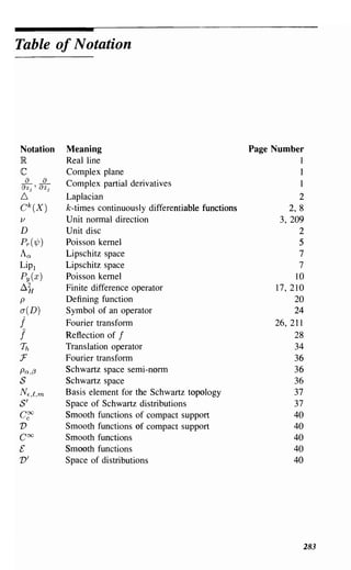
![284
Notation Meaning Page Number
[' Space of distributions 40
PK,Q Distribution semi-norm 40
8 Dirac mass 41
!*g Convolution of f and 9 43
{¢t} Friedrichs mollifiers 44
j Inverse Fourier transform of f 54
sm Symbol class 57
s;;> Symbol class 57
II IIRs Sobolev norm 57
HS Sobolev space 57
Op(p) Pseudodifferential operator 61
Tp Pseudodifferential operator 61
T* Adjoint of an operator 65
a(T) Symbol of the operator T 66
[A,B] Commutator 67
11K Symbols with support in K 68
r(x,~,y) Hormander symbol 68
Tm Hormander symbol class 69
Asymptotic expansion 69
rj Fourier transform in jth variable 69
tp Transpose of P 77
M¢ Multiplication operator 78
sing supp u Singular support of a distribution 78
8ij Kronecker delta 79
aL, aprin, ap Leading or principal symbol 88, 119,219
P(D) Partial differential operator 95
IR~ Upper half-space 95
Bj Boundary operator 95
Dj Normalized derivative 115
vO Restriction of v to the half space 116
o Tensor product 116
¢a Mobius transformation 128
A 2 (O) Bergman space 131
K(z, (), Kn(z, () Bergman kernel 132, 135
JacIR Real Jacobian matrix 136
Jace Complex Jacobian matrix 136
J Complex Jacobian matrix 136
A(O) holomorphic functions, continuous on n 138](https://image.slidesharecdn.com/partialdifferentialequationsandcomplexanalysis-121120212851-phpapp02/85/Partial-differential-equations-and-complex-analysis-295-320.jpg)
![Bibliography
[ARO] N. Aronszajn, Theory of reproducing kernels, Trans. Am. Math. Soc.
68(1950), 337-404.
[BAC] G. Bachman, Elements of Abstract Harmonic Analysis, Academic
Press, 1964.
[BAR] D. Barrett, Regularity of the Bergman projection on domains with trans-
verse symmetries, Math. Annalen 258(1982), 441-446.
[BEA 1] R. Beals, A general calculus of pseudo-differential operators, Duke
Math. J. 42(1975), 1-42.
[BEA2] R. Beals, Characterization of pseudodifferential operators and applica-
tions, Duke J. 44(1977), 45-57; correction, ibid. 46(1979), 215.
[BEA3] R. Beals, Weighted distribution spaces and pseudodifferential operators,
J. d' Analyse Mathematique 39( 1981), 131-187.
[BEFl] R. Beals and C. Fefferman, On local solvability of linear partial differ-
ential equations, Ann. Math. 97( 1973), 482-498.
[BEF2] R. Beals and C. Fefferman, Spatially inhomogeneous pseudo-
differential operators I, Comm. Pure Appl. Math. 27(1974), 1-24.
[BEA] F. Beatrous, LP estimates for extensions of holomorphic functions,
Mich. J. Math. 32(1985), 361-380.
[BEC] W. Beckner, Inequalities in Fourier analysis, Ann. Math. 102( 1975),
159-182.
[BD] E. Bedford, Proper holomorphic maps, Bull. A.M.S. 10(1984), 157-175.
[BEl] S. Bell, Analytic hypoellipticity of the a-Neumann problem and ex-
tendability of holomorphic mappings, Acta Math. 147(1981), 109-116.
[BE2] S. Bell, Biholomorphic mappings and the a problem, Ann. Math.
114(1981),103-113.
[BEB] S. Bell and H. Boas, Regularity of the Bergman projection in weakly
pseudo-convex domains, Math. Annalen 257(1981), 23-30.
[BKR] S. Bell and S. G. Krantz, Smoothness to the boundary of conformal
maps, Rocky Mt. J. Math. 17(1987),23-40.](https://image.slidesharecdn.com/partialdifferentialequationsandcomplexanalysis-121120212851-phpapp02/85/Partial-differential-equations-and-complex-analysis-298-320.jpg)
![288 BIBLIOGRAPHY
[BEL] S. Bell and E. Ligocka, A simplification and extension of Fefferman's
theorem on biholomorphic mappings, Invent. Math. 57(1980), 283-289.
[BGL] J. Bergh and J. Lofstrom, Interpolation Spaces: An Introduction,
Springer-Verlag, Berlin, 1976.
[BOl] H. Boas, Sobolev space projections in weakly pseudoconvex domains,
Trans. A.M.S. 288( 1985), 227-240.
[B02] H. Boas, Regularity of the Szego projection in weakly pseudoconvex
domains, Indiana Univ. Math. J. 34(1985),217-223.
[BOK] J. Bokobza and A. Unterberger, Sur une generalization des operateurs
de Caldero-Zygmund et des espaces H S , C. R. Acad. Sci. Paris
260(1965),3265-3267.
[BOG] A. Boggess, Tangential Cauchy-Riemann Equations and CR Manifolds
on CR Manifolds, CRC Press, Boca Raton, 1991.
[BDS] L. Boutet de Monvel and J. Sjostrand, Sur la singularite des noyaux
de Bergman et Szego, Soc. Mat. de France Asterisque 34-35(1976),
123-164.
[CAL] A. P. Calderon, unpublished lecture notes.
[CZl] A. P. Calderon and A. Zygmund, On the existence of certain singular
integrals, Acta Math. 88( 1952), 85-139.
[CZ2] A. P. Calderon and A. Zygmund, Singular integral operators and dif-
ferential equations, Am. J. Math. 79( 1957), 901-921.
[CAR] C. Caratheodory, Gesammelte Mathematische Schriften, 1955, Beck,
Munich.
[CCP] G. Carrier, M. Crook, and C. Pearson, Functions ofa Complex Variable,
McGraw-Hill, New York, 1966.
[CATl] D. Catlin, Necessary conditions for subellipticity of the a-Neumann
problem, Ann. Math. 117(1983), 147-172.
[CAT2] D. Catlin, Subelliptic estimates for the [) Neumann problem, Ann. Math.
126(1987), 131-192.
[CAT3] D. Catlin, Boundary behavior of holomorphic functions on pseudocon-
vex domains, J. Diff Geom. 15(1980), 605-625.
[CHK] D. C. Chang and S. G. Krantz, Analysis on the Heisenberg Group and
Applications, preprint.
[COL] E. Coddington and N. Levinson, Theory of Ordinary Differential Equa-
tions, McGraw-Hill, New York, 1955.
[CMB] J. F. Colombeau, New Generalized Functions and Multiplication of
Distributions, North Holland, Amsterdam and New York, 1984.
[CON] P. E. Conner, The Neumann's Problem for Differential Forms on Rie-
mannian Manifolds, Mem. Am. Math. Soc. #20, 1956.](https://image.slidesharecdn.com/partialdifferentialequationsandcomplexanalysis-121120212851-phpapp02/85/Partial-differential-equations-and-complex-analysis-299-320.jpg)
![BIBLIOGRAPHY 289
[COR] H. Cordes, On pseudodifferential operators and smoothness of special
Lie-group representations, Manuscripta Math. 28( 1979) 51-69.
[COW] H. Cordes and D. Williams, An algebra of pseudodifferential operators
with nonsmooth symbol, Pac. J. Math. 78(1978), 279-290.
[COH] R. Courant and D. Hilbert, Methods of Mathematical Physics, Inter-
science, New York, 1962.
[DAN 1] J. P. D'Angelo, Real hypersurfaces, orders of contact, and applications,
Ann. Math. 115(1982),615-637.
[DAN2] J. P. D' Angelo, Intersection theory and the a-Neumann problem, Proc.
Symp. Pure Math. 41(1984), 51-58.
[DAN3] 1. P. D'Angelo, Finite type conditions for real hypersurfaces in en.
In Complex Analysis Seminar, Springer Lecture Notes Vol. 1268,
Springer-Verlag, 1987, 83-102.
[DER] G. de Rham, Varieties Differentiables, 3rd ed., Hermann, Paris, 1973.
[DIE] K. Diederich, Uber die 1. and 2. Ableitungen der Bergmanschen Kern-
funktion und ihr Randverhalten, Math. Annalen 203(1973), 129-170.
[DF] K. Diederich and J. E. Fornress, Pseudoconvex domains with real-
analytic boundary, Ann. Math. 107(1978),371-384.
[ERD] A. Erdelyi, et aI., Higher Transcendental Functions, McGraw-Hill,
New York, 1953.
[FED] H. Federer, Geometric Measure Theory, Springer-Verlag, Berlin, 1969.
[FEF1] C. Fefferman, The Bergman kernel and biholomorphic mappings of
pseudoconvex domains, Invent. Math. 26(1974), 1-65.
[FEG] C. Fefferman, The uncertainty principle, Bull. A.M.S. 9(1983), 129-
206.
[FKP] R. Fefferman, C. Kenig, and J. Pipher, preprint.
[FOL] G. B. Folland, Spherical harmonic expansion of the Poisson-Szego
kernel for the ball, Proc. Am. Math. Soc. 47(1975),401-408.
[FOK] G. B. Folland and J. J. Kohn, The Neumann Problem for the Cauchy-
Riemann Complex, Princeton University Press, Princeton, NJ, 1972.
[GAB 1] P. Garabedian, Partial Differential Equations, Wiley, New York, 1964.
[GAB2] P. Garabedian, An unsolvable equation, Proc. A.M.S. 25( 1970), 207-
208.
[GIL] P. Gilkey, The Index Theorem and the Heat Equation, Publish or Perish
Press, Boston, 1974.
[RGR 1] C. Robin Graham, The Dirichlet problem for the Bergman Laplacian I,
Communications in Partial Differential Equations 8(1983), 433-476;
part II, ibid. 8(1983),563-641.](https://image.slidesharecdn.com/partialdifferentialequationsandcomplexanalysis-121120212851-phpapp02/85/Partial-differential-equations-and-complex-analysis-300-320.jpg)
![290 BIBLIOGRAPHY
[GRL] C. Robin Graham and J. M. Lee, Smooth solutions of degenerate Lapla-
cians on strictly pseudoconvex domains, Duke J. Math. 57( 1988), 697-
720.
[GRE] P. Greiner, Subelliptic estimates for the a-Neumann problem in C2 , J.
Diff. Geom. 9(1974),239-250.
[GRS] P. Greiner and E. M. Stein, Estimates for the a-Neumann Problem,
Princeton University Press, Princeton, 1977.
[GRU] V. Grushin, A certain example of a differential equation without so-
lutions, Mat. Zametki 1O( 1971), 125-8; transl. Math. Notes 1O( 1971),
499-501.
[GUP] M. de Guzman and I. Peral, Fourier Analysis, Proceedings of the EI
Escorial Conference, Asociacion Matematica Espanola, 1979.
[HAD] J. Hadamard, Le probleme de Cauchy et les equations aux derivees
partielles lineaires hyperboliques, Paris, 1932.
[HAS] M. Hakim and N. Sibony, Spectre de A(O) pour des domaines bomes
faiblement pseudoconvexes reguliers, J. Funct. Anal. 37(1980), 127-
135.
[HEI] M. Heins, Complex Function Theory, Academic Press, New York,
1968.
[HEL] S. Helgason, Differential Geometry and Symmetric Spaces, Academic
Press, New York, 1962.
[HIR] M. Hirsch, Differential Topology, Springer-Verlag, Berlin, 1976.
[HOR1] L. Hormander, Linear Partial Differential Equations, Springer-Verlag,
Berlin, 1969.
[HOR2] L. Hormander, Pseudo-differential operators, Comm. Pure Appl. Math.
18(1965),501-517.
[HOR3] L. Hormander, Pseudo-differential operators and non-elliptic boundary
problems, Ann. Math. 83«1966), 129-209.
[HOR4] L. Hormander, The Analysis of Linear Partial Differential Operators,
in four volumes, Springer-Verlag, Berlin, 1983-1985.
[HOR5] L. Hormander, The Weyl calculus of pseudo-differential operators,
Comm. Pure Appl. Math. 32(1979), 359-443.
[INCE] E. L. Ince, Ordinary Differential Equations, Longmans, Green, and
Co., London and New York, 1927.
[JAT] H. Jacobowitz and F. Treves, Nowhere solvable homogeneous partial
differential equations, Bull. A.M.S. 8( 1983), 467-469.
[KAN] S. Kaneyuki, Homogeneous Domains and Siegel Domains, Springer
Lecture Notes no. 241 , Springer-Verlag, Berlin, 1971.](https://image.slidesharecdn.com/partialdifferentialequationsandcomplexanalysis-121120212851-phpapp02/85/Partial-differential-equations-and-complex-analysis-301-320.jpg)
![BIBLIOGRAPHY 291
[KAT] Y. Katznelson, An Introduction to Harmonic Analysis, Wiley, New
York, 1968.
[KEL1] O. D. Kellogg, Foundations of Potential Theory, Springer-Verlag,
Berlin, 1929.
[KEL2] O. D. Kellogg, Harmonic functions and Green's integral, Trans. Am.
Math. Soc. 13(1912), 109-132.
[KER1] N. Kerzman, A Monge-Ampere equation in complex analysis, Proc.
Symp. Pure Math. , Vol. 30, Part 1, American Mathematical Society,
Providence, RI, 1977, 161-168.
[KER2] N. Kerzman, The Bergman kernel function. Differentiability at the
boundary, Math. Annalen 195(1972), 149-158.
[KOM] S. Kobayashi and K. Nomizu, Foundations of Differential Geometry,
Vols. I and II, Interscience, New York, 1963, 1969.
[KOHl] J. J. Kohn, Harmonic integrals on strongly pseudoconvex manifolds I,
Ann. Math. 78(1963), 112-148; II, ibid. 79(1964),450-472.
[KOH2] J. J. Kohn, Methods of partial differential equations in complex analy-
sis, Proc. Symp. Pure Math., Vol. 30, American Mathematical Society,
Providence, RI, 1977,215-237.
[KOH3] J. J. Kohn, A survey of the a-Neumann problem, Proceedings of Sym-
posia in Pure Math. 41(1984), 137-145.
[KON1] J. J. Kohn and L. Nirenberg, On the algebra of pseudo-differential
operators, Comm. Pure Appl. Math. 18(1965),269-305.
[KON2] J. J. Kohn and L. Nirenberg, Non-coercive boundary value problems,
Comm. Pure and Appl. Math. 18(1965),443-492.
[KOV] A. Koranyi and S. Vagi, Singular integrals in homogeneous spaces
and some problems of classical analysis, Ann. Scuola Norm. Sup. Pisa
25(1971), 575-648.
[KR1] S. G. Krantz, Function Theory of Several Complex Variables, 2nd Ed.,
Wadsworth Publishing, Belmont, 1992.
[KR2] S. G. Krantz, Lipschitz spaces, smoothness of functions, and approxi-
mation theory, Expositiones Math. 3(1983), 193-260.
[KR3] S. G. Krantz, Geometric Lipschitz spaces and applications to complex
function theory and nilpotent groups, J. Funct. Anal. 34( 1979), 456-
471.
[KR4] S. G. Krantz, Characterization of various domains of holomorphy via a
estimates and applications to a problem of Kohn, Ill. J. Math. 23( 1979),
267-286.
[KRP] S. G. Krantz and H. R. Parks, A Primer of Real Analytic Functions,
Birkhauser, Basel, 1992, to appear.](https://image.slidesharecdn.com/partialdifferentialequationsandcomplexanalysis-121120212851-phpapp02/85/Partial-differential-equations-and-complex-analysis-302-320.jpg)
![292 BIBLIOGRAPHY
[LEWl] H. Lewy, On the local character of the solutions of an atypical linear
differential equation in three variables and a related theorem for regular
functions of two complex variables, Ann. Math. 64(1956),514-522.
[LEW2] H. Lewy, An example of a smooth linear partial differential equation
without solution, Ann. Math. 66(1957), 155-158.
[LUM] Lumer, Expaces de Hardy en plusieurs variables complexes, C. R. Acad.
Sci. Paris Sere A-B 273(1971), A151-A154.
[MEY] Y. Meyer, Estimations £2 pour les operateurs pseudo-differentiels,
Seminaire d' Analyse Harmonique (1977/1978), 47-53, Publ. Math. Or-
say 78, 12, Univ. Paris XI, Orsay, 1978.
[MIK1] S. G. Mikhlin, On the multipliers of Fourier integrals, Dokl. Akad.
Nauk SSSR 109(1956), 701-703.
[MIK2] S. G. Mikhlin, Multidimensional Singular Integral Equations, Pergam-
mon Press, New York, 1965.
[MIS] B. Mityagin and E. M. Semenov, The space C k is not an interpolation
space between C and Cn,O < k < n, Sov. Math. Dokl. 17(1976),
778-782.
[MOR] C. B. Morrey, Multiple Integrals in the Calculus of Variations,
Springer-Verlag, Berlin, 1966.
[MOS] J. Moser, On Harnack's theorem for elliptic differential equations,
Comm. Pure Appl. Math. 14(1961),577-591.
[NIR] L. Nirenberg, Lectures on Linear Partial Differential Equations, Amer-
ican Mathematical Society, Providence, RI, 1973.
[NTR] L. Nirenberg and F. Treves, On local solvability of linear partial dif-
ferential equations I. Necessary conditions; II. Sufficient Conditions,
Comm. Pure and Appl. Math. 23(1970), 1-38; 459-510; Correction,
ibid. 24(1971), 279-288.
[OSG] W. F. Osgood, Lehrbuch der Funktionentheorie, vols. 1 and 2,
B. G. Teubner, Leipzig, 1912.
[PAl] P. Painleve, Sur les lignes singulieres des functions analytiques, These,
Gauthier-Villars, Paris, 1887.
[PEE] J. Peetre, Rectifications a I' article "Une caracterisation abstraite des
operateurs differentiels', Math. Scand. 8(1960),116-120.
[RAN] R. M. Range, Holomorphic Functions and Integral Representations in
Several Complex Variables, Springer-Verlag, Berlin, 1986.
[RIEl M. Riesz, L'integrale de Riemann-Liouville et Ie probleme de Cauchy,
Acta Math. 81(1949), 1-223.
[ROM] S. Roman, The formula of Faa di Bruno, Am. Math. Monthly 87(1980),
805-809.](https://image.slidesharecdn.com/partialdifferentialequationsandcomplexanalysis-121120212851-phpapp02/85/Partial-differential-equations-and-complex-analysis-303-320.jpg)
![BIBLIOGRAPHY 293
[RUD1] W. Rudin, Principles of Mathematical Analysis, 3rd Ed., McGraw-Hill, New
York, 1976.
[RUD2] W. Rudin, Function Theory in the Unit Ball of en, Springer-Verlag, Berlin,
1980.
[RUD3] W. Rudin, Real and Complex Analysis, McGraw-Hill, New York, 1966.
[SCH] L. Schwartz, Theorie des Distributions, I, II, Hennann, Paris, 1950-51.
[SPE] D. C. Spencer, Overdetennined systems of iinear partial differential equations,
Bull. Am. Math. Soc. 75(1969), 179-239.
[STSI] E. M. Stein, Singular Integrals and Differentiability Properties of Functions,
Princeton University Press, 1970.
[STBV] E. M. Stein, The Boundary Behavior of Holomorphic Functions of Several
Complex Variables, Princeton University Press, Princeton, 1972.
[STW] E. M. Stein and G. Weiss, Introduction to Fourier Analysis on Euclidean Spaces,
Princeton University Press, Princeton, 1971.
[STR] K. Stromberg, An Introduction to Classical Real Analysis, Wadsworth, Belmont,
1981.
[TAR] D. Tartakoff, The local real analyticity of solutions to Db and the a-Neumann
problem, Acta Math. 145(1980), 177-204.
[TAY] M. Taylor, Pseudodifferential Operators, Princeton University Press, Princeton,
1981.
[TRE1] F. Treves, Analytic hypo-ellipticity of a class of pseudodifferential operators
with double characteristics and applications to thea-
Neumann problem, Comm.
Partial Diff. Eqs. 3:6-7(1978),475-642.
[TRE2] F. Treves, Introduction to Pseudodifferential and Fourier Integral Operators, 2
vols., Plenum, New York, 1980.
[TRI] H. Triebel, Theory of Function Spaces, Birkhauser, Basel and Boston, 1983.
[UNT] A. Unterberger, Resolution d'equations aux derivees partielles dans les espaces
de distributions d'ordre de regularite variable, Ann. Inst Fourier 21(1971) 85-
128.
[WEL] R. O. Wells, Differential Analysis on Complex Manifolds, 2nd ed., Springer-
Verlag, 1979.
[WHW] Whittaker and Watson, A Course of Modern Analysis, 4th ed., Cambridge Univ.
Press, London, 1935.
[WID] H. Widonl, Lectures on Integral Equations, Van Nostrand Reinhold, New York,
1969.
[ZAU] E. Zauderer, Partial Differential Equations of Applied Mathematics, John Wiley
and Sons, New York, 1
[ZYG] A. Zygmund, Trigonometric Series, Cambridge University Press, Cambridge,
UK, 1968.](https://image.slidesharecdn.com/partialdifferentialequationsandcomplexanalysis-121120212851-phpapp02/85/Partial-differential-equations-and-complex-analysis-304-320.jpg)


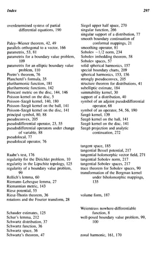

The document summarizes the Dirichlet problem for the Laplace equation on the unit disc D. The Dirichlet problem asks us to find a function U that is harmonic (satisfies the Laplace equation) in D, continuous on D, and matches given boundary values φ on the boundary of D. The solution can be written as a Fourier series involving the basis functions zn on D, which match the boundary values φn on ∂D. This represents the unique solution in L2. Furthermore, the series converges uniformly on compact subsets of D as the radius r approaches 1.


