The document consists of lecture handouts on operating systems, covering various topics including definitions, services, process management, synchronization, CPU scheduling, deadlock, memory management, file systems, and input/output principles. It provides detailed sections on processes, threads, IPC, deadlock modeling, memory allocation techniques, file system structures, and I/O hardware principles. The handouts serve as a comprehensive study resource for understanding the functions and management of operating systems.

1. Operating Systems
Lecture Handouts
Wang Xiaolin
wx672ster+os@gmail.com
April 9, 2016
Contents
1 Introduction 5
1.1 What’s an Operating System . . . . . . . . . . . . . . . . . . . . . . . . . . . . . . 5
1.2 OS Services . . . . . . . . . . . . . . . . . . . . . . . . . . . . . . . . . . . . . . . . 8
1.3 Hardware . . . . . . . . . . . . . . . . . . . . . . . . . . . . . . . . . . . . . . . . . . 9
1.4 Bootstrapping . . . . . . . . . . . . . . . . . . . . . . . . . . . . . . . . . . . . . . . 12
1.5 Interrupt . . . . . . . . . . . . . . . . . . . . . . . . . . . . . . . . . . . . . . . . . . 13
1.6 System Calls . . . . . . . . . . . . . . . . . . . . . . . . . . . . . . . . . . . . . . . . 14
2 Process And Thread 18
2.1 Processes . . . . . . . . . . . . . . . . . . . . . . . . . . . . . . . . . . . . . . . . . . 18
2.1.1 What’s a Process . . . . . . . . . . . . . . . . . . . . . . . . . . . . . . . . . 18
2.1.2 PCB . . . . . . . . . . . . . . . . . . . . . . . . . . . . . . . . . . . . . . . . . 19
2.1.3 Process Creation . . . . . . . . . . . . . . . . . . . . . . . . . . . . . . . . . 19
2.1.4 Process State . . . . . . . . . . . . . . . . . . . . . . . . . . . . . . . . . . . 21
2.1.5 CPU Switch From Process To Process . . . . . . . . . . . . . . . . . . . . . 21
2.2 Threads . . . . . . . . . . . . . . . . . . . . . . . . . . . . . . . . . . . . . . . . . . . 22
2.2.1 Processes vs. Threads . . . . . . . . . . . . . . . . . . . . . . . . . . . . . . 22
2.2.2 Why Thread? . . . . . . . . . . . . . . . . . . . . . . . . . . . . . . . . . . . . 23
2.2.3 Thread Characteristics . . . . . . . . . . . . . . . . . . . . . . . . . . . . . . 24
2.2.4 POSIX Threads . . . . . . . . . . . . . . . . . . . . . . . . . . . . . . . . . . 25
2.2.5 User-Level Threads vs. Kernel-level Threads . . . . . . . . . . . . . . . . 27
2.2.6 Linux Threads . . . . . . . . . . . . . . . . . . . . . . . . . . . . . . . . . . . 29
3 Process Synchronization 32
3.1 IPC . . . . . . . . . . . . . . . . . . . . . . . . . . . . . . . . . . . . . . . . . . . . . . 33
3.2 Shared Memory . . . . . . . . . . . . . . . . . . . . . . . . . . . . . . . . . . . . . . 33
3.3 Race Condition and Mutual Exclusion . . . . . . . . . . . . . . . . . . . . . . . . 35
3.4 Semaphores . . . . . . . . . . . . . . . . . . . . . . . . . . . . . . . . . . . . . . . . 39
3.5 Monitors . . . . . . . . . . . . . . . . . . . . . . . . . . . . . . . . . . . . . . . . . . 47
3.6 Message Passing . . . . . . . . . . . . . . . . . . . . . . . . . . . . . . . . . . . . . 47
3.7 Classical IPC Problems . . . . . . . . . . . . . . . . . . . . . . . . . . . . . . . . . . 49
3.7.1 The Dining Philosophers Problem . . . . . . . . . . . . . . . . . . . . . . . 49
3.7.2 The Readers-Writers Problem . . . . . . . . . . . . . . . . . . . . . . . . . . 52
3.7.3 The Sleeping Barber Problem . . . . . . . . . . . . . . . . . . . . . . . . . . 52
1

2. CONTENTS
4 CPU Scheduling 54
4.1 Process Scheduling Queues . . . . . . . . . . . . . . . . . . . . . . . . . . . . . . . 54
4.2 Scheduling . . . . . . . . . . . . . . . . . . . . . . . . . . . . . . . . . . . . . . . . . 55
4.3 Process Behavior . . . . . . . . . . . . . . . . . . . . . . . . . . . . . . . . . . . . . 56
4.4 Process Classification . . . . . . . . . . . . . . . . . . . . . . . . . . . . . . . . . . 56
4.5 Process Schedulers . . . . . . . . . . . . . . . . . . . . . . . . . . . . . . . . . . . . 57
4.6 Scheduling In Batch Systems . . . . . . . . . . . . . . . . . . . . . . . . . . . . . . 57
4.7 Scheduling In Interactive Systems . . . . . . . . . . . . . . . . . . . . . . . . . . . 58
4.8 Thread Scheduling . . . . . . . . . . . . . . . . . . . . . . . . . . . . . . . . . . . . 59
4.9 Linux Scheduling . . . . . . . . . . . . . . . . . . . . . . . . . . . . . . . . . . . . . 59
4.9.1 Completely Fair Scheduling . . . . . . . . . . . . . . . . . . . . . . . . . . . 61
5 Deadlock 63
5.1 Resources . . . . . . . . . . . . . . . . . . . . . . . . . . . . . . . . . . . . . . . . . 63
5.2 Introduction to Deadlocks . . . . . . . . . . . . . . . . . . . . . . . . . . . . . . . . 64
5.3 Deadlock Modeling . . . . . . . . . . . . . . . . . . . . . . . . . . . . . . . . . . . . 65
5.4 Deadlock Detection and Recovery . . . . . . . . . . . . . . . . . . . . . . . . . . . 66
5.5 Deadlock Avoidance . . . . . . . . . . . . . . . . . . . . . . . . . . . . . . . . . . . 69
5.6 Deadlock Prevention . . . . . . . . . . . . . . . . . . . . . . . . . . . . . . . . . . . 71
5.7 The Ostrich Algorithm . . . . . . . . . . . . . . . . . . . . . . . . . . . . . . . . . . 72
6 Memory Management 72
6.1 Background . . . . . . . . . . . . . . . . . . . . . . . . . . . . . . . . . . . . . . . . 73
6.2 Contiguous Memory Allocation . . . . . . . . . . . . . . . . . . . . . . . . . . . . . 82
6.3 Virtual Memory . . . . . . . . . . . . . . . . . . . . . . . . . . . . . . . . . . . . . . 83
6.3.1 Paging . . . . . . . . . . . . . . . . . . . . . . . . . . . . . . . . . . . . . . . . 84
6.3.2 Demand Paging . . . . . . . . . . . . . . . . . . . . . . . . . . . . . . . . . . 91
6.3.3 Copy-on-Write . . . . . . . . . . . . . . . . . . . . . . . . . . . . . . . . . . . 92
6.3.4 Memory mapped files . . . . . . . . . . . . . . . . . . . . . . . . . . . . . . 92
6.3.5 Page Replacement Algorithms . . . . . . . . . . . . . . . . . . . . . . . . . 93
6.3.6 Allocation of Frames . . . . . . . . . . . . . . . . . . . . . . . . . . . . . . . 96
6.3.7 Thrashing And Working Set Model . . . . . . . . . . . . . . . . . . . . . . . 97
6.3.8 Other Issues . . . . . . . . . . . . . . . . . . . . . . . . . . . . . . . . . . . . 100
6.3.9 Segmentation . . . . . . . . . . . . . . . . . . . . . . . . . . . . . . . . . . . 103
7 File Systems 111
7.1 File System Structure . . . . . . . . . . . . . . . . . . . . . . . . . . . . . . . . . . 111
7.2 Files . . . . . . . . . . . . . . . . . . . . . . . . . . . . . . . . . . . . . . . . . . . . . 112
7.3 Directories . . . . . . . . . . . . . . . . . . . . . . . . . . . . . . . . . . . . . . . . . 116
7.4 File System Implementation . . . . . . . . . . . . . . . . . . . . . . . . . . . . . . 117
7.4.1 Basic Structures . . . . . . . . . . . . . . . . . . . . . . . . . . . . . . . . . . 117
7.4.2 Implementing Files . . . . . . . . . . . . . . . . . . . . . . . . . . . . . . . . 118
7.4.3 Implementing Directories . . . . . . . . . . . . . . . . . . . . . . . . . . . . 129
7.4.4 Shared Files . . . . . . . . . . . . . . . . . . . . . . . . . . . . . . . . . . . . 132
7.4.5 Disk Space Management . . . . . . . . . . . . . . . . . . . . . . . . . . . . . 134
7.5 Ext2 File System . . . . . . . . . . . . . . . . . . . . . . . . . . . . . . . . . . . . . 136
7.5.1 Ext2 File System Layout . . . . . . . . . . . . . . . . . . . . . . . . . . . . . 136
7.5.2 Ext2 Block groups . . . . . . . . . . . . . . . . . . . . . . . . . . . . . . . . . 137
7.5.3 Ext2 Inode . . . . . . . . . . . . . . . . . . . . . . . . . . . . . . . . . . . . . 139
7.5.4 Ext2 Superblock . . . . . . . . . . . . . . . . . . . . . . . . . . . . . . . . . . 140
7.5.5 Ext2 Directory . . . . . . . . . . . . . . . . . . . . . . . . . . . . . . . . . . . 141
7.6 Vitural File Systems . . . . . . . . . . . . . . . . . . . . . . . . . . . . . . . . . . . 141
2

3. REFERENCES
8 Input/Output 150
8.1 Principles of I/O Hardware . . . . . . . . . . . . . . . . . . . . . . . . . . . . . . . 150
8.1.1 Programmed I/O . . . . . . . . . . . . . . . . . . . . . . . . . . . . . . . . . . 155
8.1.2 Interrupt-Driven I/O . . . . . . . . . . . . . . . . . . . . . . . . . . . . . . . 157
8.1.3 Direct Memory Access (DMA) . . . . . . . . . . . . . . . . . . . . . . . . . 157
8.2 I/O Software Layers . . . . . . . . . . . . . . . . . . . . . . . . . . . . . . . . . . . 159
8.2.1 Interrupt Handlers . . . . . . . . . . . . . . . . . . . . . . . . . . . . . . . . 160
8.2.2 Device Drivers . . . . . . . . . . . . . . . . . . . . . . . . . . . . . . . . . . . 160
8.2.3 Device-Independent I/O Software . . . . . . . . . . . . . . . . . . . . . . . 161
8.2.4 User-Space I/O Software . . . . . . . . . . . . . . . . . . . . . . . . . . . . . 161
8.3 Disks . . . . . . . . . . . . . . . . . . . . . . . . . . . . . . . . . . . . . . . . . . . . 162
8.3.1 Disk Scheduling . . . . . . . . . . . . . . . . . . . . . . . . . . . . . . . . . . 162
8.3.2 RAID Structure . . . . . . . . . . . . . . . . . . . . . . . . . . . . . . . . . . 165
References
[1] M.J. Bach. The design of the UNIX operating system. Prentice-Hall software series.
Prentice-Hall, 1986.
[2] D.P. Bovet and M. Cesatı́. Understanding The Linux Kernel. 3rd ed. O’Reilly, 2005.
[3] Randal E. Bryant and David R. O’Hallaron. Computer Systems: A Programmer’s Per-
spective. 2nd ed. USA: Addison-Wesley Publishing Company, 2010.
[4] Rémy Card, Theodore Ts’o, and Stephen Tweedie. “Design and Implementation of
the Second Extended Filesystem”. In: Dutch International Symposium on Linux (1996).
[5] Allen B. Downey. The Little Book of Semaphores. greenteapress.com, 2008.
[6] M. Gorman. Understanding the Linux Virtual Memory Manager. Prentice Hall, 2004.
[7] Research Computing Support Group. “Understanding Memory”. In: University of
Alberta (2010). http://cluster.srv.ualberta.ca/doc/.
[8] Sandeep Grover. “Linkers and Loaders”. In: Linux Journal (2002).
[9] Intel. INTEL 80386 Programmer’s Reference Manual. 1986.
[10] John Levine. Linkers and Loaders. Morgan-Kaufman, Oct. 1999.
[11] R. Love. Linux Kernel Development. Developer’s Library. Addison-Wesley, 2010.
[12] W. Mauerer. Professional Linux Kernel Architecture. John Wiley & Sons, 2008.
[13] David Morgan. Analyzing a filesystem. 2012.
[14] Abhishek Nayani, Mel Gorman, and Rodrigo S. de Castro. Memory Management in
Linux: Desktop Companion to the Linux Source Code. Free book, 2002.
[15] Dave Poirier. The Second Extended File System Internal Layout. Web, 2011.
[16] David A Rusling. The Linux Kernel. Linux Documentation Project, 1999.
[17] Silberschatz, Galvin, and Gagne. Operating System Concepts Essentials. John Wiley
& Sons, 2011.
[18] Wiliam Stallings. Operating Systems: Internals and Design Principles. 7th ed. Pren-
tice Hall, 2011.
[19] Andrew S. Tanenbaum. Modern Operating Systems. 3rd. Prentice Hall Press, 2007.
[20] K. Thompson. “Unix Implementation”. In: Bell System Technical Journal 57 (1978),
pp. 1931–1946.
3

4. REFERENCES
[21] Wikipedia. Assembly language — Wikipedia, The Free Encyclopedia. [Online; ac-
cessed 11-May-2015]. 2015.
[22] Wikipedia. Compiler — Wikipedia, The Free Encyclopedia. [Online; accessed 11-
May-2015]. 2015.
[23] Wikipedia. Dining philosophers problem — Wikipedia, The Free Encyclopedia. [On-
line; accessed 11-May-2015]. 2015.
[24] Wikipedia. Directed acyclic graph — Wikipedia, The Free Encyclopedia. [Online;
accessed 12-May-2015]. 2015.
[25] Wikipedia. Dynamic linker — Wikipedia, The Free Encyclopedia. 2012.
[26] Wikipedia. Executable and Linkable Format — Wikipedia, The Free Encyclopedia.
[Online; accessed 12-May-2015]. 2015.
[27] Wikipedia. File Allocation Table — Wikipedia, The Free Encyclopedia. [Online; ac-
cessed 12-May-2015]. 2015.
[28] Wikipedia. File descriptor — Wikipedia, The Free Encyclopedia. [Online; accessed
12-May-2015]. 2015.
[29] Wikipedia. Inode — Wikipedia, The Free Encyclopedia. [Online; accessed 21-February-
2015]. 2015.
[30] Wikipedia. Linker (computing) — Wikipedia, The Free Encyclopedia. [Online; ac-
cessed 11-May-2015]. 2015.
[31] Wikipedia. Loader (computing) — Wikipedia, The Free Encyclopedia. 2012.
[32] Wikipedia. Open (system call) — Wikipedia, The Free Encyclopedia. [Online; ac-
cessed 12-May-2015]. 2014.
[33] Wikipedia. Page replacement algorithm — Wikipedia, The Free Encyclopedia. [On-
line; accessed 11-May-2015]. 2015.
[34] Wikipedia. Process (computing) — Wikipedia, The Free Encyclopedia. [Online; ac-
cessed 21-February-2015]. 2014.
[35] 邹恒明. 计算机的心智：操作系统之哲学原理. 机械工业出版社, 2009.
4

5. 1 Introduction
Course Web Site
Course web site: http://cs2.swfu.edu.cn/moodle
Lecture slides: http://cs2.swfu.edu.cn/∼wx672/lecture_notes/os/slides/
Source code: http://cs2.swfu.edu.cn/∼wx672/lecture_notes/os/src/
Sample lab report: http://cs2.swfu.edu.cn/∼wx672/lecture_notes/os/sample-report/
1.1 What’s an Operating System
What’s an Operating System?
• “Everything a vendor ships when you order an operating system”
• It’s the program that runs all the time
• It’s a resource manager
- Each program gets time with the resource
Each program gets space on the resource
• It’s a control program
- Controls execution of programs to prevent errors and improper use of the com-
puter
• No universally accepted definition
5

6. 1.1 What’s an Operating System
Hardware
Hardware control
Device drivers
Character
devices
Block
devices
Buffer
cache
File subsystem
VFS
NFS · · · Ext2 VFAT
Process control
subsystem
Inter-process
communication
Scheduler
Memory
management
System call interface
Libraries
Kernel level
Hardware level
User level
Kernel level
User programs
trap
trap
6

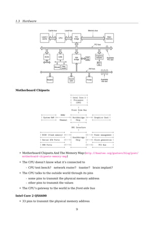
7. 1.1 What’s an Operating System
Abstractions
To hide the complexity of the actual implementationsSection 1.10 Summary 25
Figure 1.18
Some abstractions pro-
vided by a computer
system. A major theme
in computer systems is to
provide abstract represen-
tations at different levels to
hide the complexity of the
actual implementations.
Main memory I/O devicesProcessorOperating system
Processes
Virtual memory
Files
Virtual machine
Instruction set
architecture
sor that performs just one instruction at a time. The underlying hardware is far
more elaborate, executing multiple instructions in parallel, but always in a way
that is consistent with the simple, sequential model. By keeping the same execu-
tion model, different processor implementations can execute the same machine
code, while offering a range of cost and performance.
On the operating system side, we have introduced three abstractions: files as
an abstraction of I/O, virtual memory as an abstraction of program memory, and
processes as an abstraction of a running program. To these abstractions we add
a new one: the virtual machine, providing an abstraction of the entire computer,
including the operating system, the processor, and the programs. The idea of a
virtual machine was introduced by IBM in the 1960s, but it has become more
prominent recently as a way to manage computers that must be able to run
programs designed for multiple operating systems (such as Microsoft Windows,
MacOS, and Linux) or different versions of the same operating system.
We will return to these abstractions in subsequent sections of the book.
1.10 Summary
A computer system consists of hardware and systems software that cooperate
to run application programs. Information inside the computer is represented as
groups of bits that are interpreted in different ways, depending on the context.
Programs are translated by other programs into different forms, beginning as
ASCII text and then translated by compilers and linkers into binary executable
files.
Processors read and interpret binary instructions that are stored in main
memory. Since computers spend most of their time copying data between memory,
I/O devices, and the CPU registers, the storage devices in a system are arranged
in a hierarchy, with the CPU registers at the top, followed by multiple levels
of hardware cache memories, DRAM main memory, and disk storage. Storage
devices that are higher in the hierarchy are faster and more costly per bit than
those lower in the hierarchy. Storage devices that are higher in the hierarchy serve
as caches for devices that are lower in the hierarchy. Programmers can optimize
the performance of their C programs by understanding and exploiting the memory
hierarchy.
See also: [3, Sec. 1.9.2, The Importance of Abstractions in Computer Systems]
System Goals
Convenient vs. Efficient
• Convenient for the user — for PCs
• Efficient — for mainframes, multiusers
• UNIX
- Started with keyboard + printer, none paid to convenience
- Now, still concentrating on efficiency, with GUI support
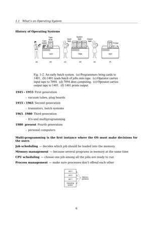
History of Operating Systems
1401 7094 1401
(a) (b) (c) (d) (e) (f)
Card
reader
Tape
drive Input
tape
Output
tape
System
tape
Printer
Fig. 1-2. An early batch system. (a) Programmers bring cards to
1401. (b) 1401 reads batch of jobs onto tape. (c) Operator carries
input tape to 7094. (d) 7094 does computing. (e) Operator carries
output tape to 1401. (f) 1401 prints output.
1945 - 1955 First generation
- vacuum tubes, plug boards
1955 - 1965 Second generation
- transistors, batch systems
1965 - 1980 Third generation
7

8. 1.2 OS Services
- ICs and multiprogramming
1980 - present Fourth generation
- personal computers
Multi-programming is the first instance where the OS must make decisions for
the users
Job scheduling — decides which job should be loaded into the memory.
Memory management — because several programs in memory at the same time
CPU scheduling — choose one job among all the jobs are ready to run
Process management — make sure processes don’t offend each other
Job 3
Job 2
Job 1
Operating
system
Memory
partitions
Fig. 1-4. A multiprogramming system with three jobs in memory.
The Operating System Zoo
• Mainframe OS
• Server OS
• Multiprocessor OS
• Personal computer OS
• Real-time OS
• Embedded OS
• Smart card OS
1.2 OS Services
OS Services
Like a government
Helping the users:
• User interface
• Program execution
• I/O operation
• File system manipulation
• Communication
• Error detection
8

9. 1.3 Hardware
Keeping the system efficient:
• Resource allocation
• Accounting
• Protection and security
A Computer System
Banking
system
Airline
reservation
Operating system
Web
browser
Compilers Editors
Application programs
Hardware
System
programs
Command
interpreter
Machine language
Microarchitecture
Physical devices
Fig. 1-1. A computer system consists of hardware, system pro-
grams, and application programs.
1.3 Hardware
CPU Working Cycle
Fetch
unit
Decode
unit
Execute
unit
1. Fetch the first instruction from memory
2. Decode it to determine its type and operands
3. execute it
Special CPU Registers
Program counter(PC): keeps the memory address of the next instruction to be fetched
Stack pointer(SP): points to the top of the current stack in memory
Program status(PS): holds
- condition code bits
- processor state
9

10. 1.3 Hardware
System Bus
Monitor
Keyboard
Floppy
disk drive
Hard
disk drive
Hard
disk
controller
Floppy
disk
controller
Keyboard
controller
Video
controller
MemoryCPU
Bus
Fig. 1-5. Some of the components of a simple personal computer.
Address Bus: specifies the memory locations (addresses) for the data transfers
Data Bus: holds the data transfered. bidirectional
Control Bus: contains various lines used to route timing and control signals throughout
the system
Controllers and Peripherals
• Peripherals are real devices controlled by controller chips
• Controllers are processors like the CPU itself, have control registers
• Device driver writes to the registers, thus control it
• Controllers are connected to the CPU and to each other by a variety of buses
ISA
bridge
Modem
Mouse
PCI
bridgeCPU
Main
memory
SCSI USB
Local bus
Sound
card
Printer Available
ISA slot
ISA bus
IDE
disk
Available
PCI slot
Key-
board
Mon-
itor
Graphics
adaptor
Level 2
cache
Cache bus Memory bus
PCI bus
Fig. 1-11. The structure of a large Pentium systemMotherboard Chipsets
10

11. 1.3 Hardware
Intel Core 2
(CPU)
Front
Side
Bus
North bridge
Chip
DDR2System RAM Graphics Card
DMI
Interface
South bridge
Chip
Serial ATA Ports Clock Generation
BIOS
USB Ports
Power Management
PCI Bus
See also: Motherboard Chipsets And The Memory Map1
• The CPU doesn’t know what it’s connected to
- CPU test bench? network router? toaster? brain implant?
• The CPU talks to the outside world through its pins
- some pins to transmit the physical memory address
- other pins to transmit the values
• The CPU’s gateway to the world is the front-side bus
Intel Core 2 QX6600
• 33 pins to transmit the physical memory address
- so there are 233
choices of memory locations
• 64 pins to send or receive data
- so data path is 64-bit wide, or 8-byte chunks
This allows the CPU to physically address 64GB of memory (233
× 8B)
1http://duartes.org/gustavo/blog/post/motherboard-chipsets-memory-map
11

12. 1.4 Bootstrapping
See also: Datasheet for Intel Core 2 Quad-Core Q6000 Sequence2
Some physical memory addresses are mapped away!
• only the addresses, not the spaces
• Memory holes
- 640KB ∼ 1MB
- /proc/iomem
Memory-mapped I/O
• BIOS ROM
• video cards
• PCI cards
• ...
This is why 32-bit OSes have problems using 4 gigs of RAM.
0xFFFFFFFF +--------------------+ 4GB
Reset vector | JUMP to 0xF0000 |
0xFFFFFFF0 +--------------------+ 4GB - 16B
| Unaddressable |
| memory, real mode |
| is limited to 1MB. |
0x100000 +--------------------+ 1MB
| System BIOS |
0xF0000 +--------------------+ 960KB
| Ext. System BIOS |
0xE0000 +--------------------+ 896KB
| Expansion Area |
| (maps ROMs for old |
| peripheral cards) |
0xC0000 +--------------------+ 768KB
| Legacy Video Card |
| Memory Access |
0xA0000 +--------------------+ 640KB
| Accessible RAM |
| (640KB is enough |
| for anyone - old |
| DOS area) |
0 +--------------------+ 0
What if you don’t have 4G RAM?
the northbridge
1. receives a physical memory request
2. decides where to route it
- to RAM? to video card? to ...?
- decision made via the memory address map
• When is the memory address map built? setup().
1.4 Bootstrapping
Bootstrapping
Can you pull yourself up by your own bootstraps?
A computer cannot run without first loading software but must be running before any
software can be loaded.
BIOS
Initialization
MBR Boot Loader
Earily
Kernel
Initialization
Full
Kernel
Initialization
First
User Mode
Process
BIOS Services Kernel Services
Hardware
CPU in Real Mode
Time flow
CPU in Protected Mode
Switch to
Protected Mode
2http://download.intel.com/design/processor/datashts/31559205.pdf
12

13. 1.5 Interrupt
Intel x86 Bootstrapping
1. BIOS (0xfffffff0)
« POST « HW init « Find a boot device (FD,CD,HD...) « Copy sector zero (MBR) to RAM
(0x00007c00)
2. MBR – the first 512 bytes, contains
• Small code (< 446 Bytes), e.g. GRUB stage 1, for loading GRUB stage 2
• the primary partition table (= 64 Bytes)
• its job is to load the second-stage boot loader.
3. GRUB stage 2 — load the OS kernel into RAM
4. startup
5. init — the first user-space program
|<-------------Master Boot Record (512 Bytes)------------>|
0 439 443 445 509 511
+----//-----+----------+------+------//---------+---------+
| code area | disk-sig | null | partition table | MBR-sig |
| 440 | 4 | 2 | 16x4=64 | 0xAA55 |
+----//-----+----------+------+------//---------+---------+
$ sudo hd -n512 /dev/sda
1.5 Interrupt
Why Interrupt?
While a process is reading a disk file, can we do...
while(!done_reading_a_file())
{
let_CPU_wait();
// or...
lend_CPU_to_others();
}
operate_on_the_file();
Modern OS are Interrupt Driven
HW INT by sending a signal to CPU
SW INT by executing a system call
Trap (exception) is a software-generated INT coursed by an error or by a specific request
from an user program
Interrupt vector is an array of pointers pointing to the memory addresses of interrupt
handlers. This array is indexed by a unique device number
$ less /proc/devices
$ less /proc/interrupts
13

14. 1.6 System Calls
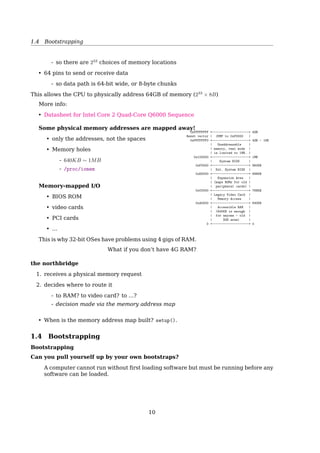
Programmable Interrupt Controllers
Interrupt
INT
IRQ 0 (clock)
IRQ 1 (keyboard)
IRQ 3 (tty 2)
IRQ 4 (tty 1)
IRQ 5 (XT Winchester)
IRQ 6 (floppy)
IRQ 7 (printer)
IRQ 8 (real time clock)
IRQ 9 (redirected IRQ 2)
IRQ 10
IRQ 11
IRQ 12
IRQ 13 (FPU exception)
IRQ 14 (AT Winchester)
IRQ 15
ACK
Master
interrupt
controller
INT
ACK
Slave
interrupt
controller
INT
CPU
INTA
Interrupt
ack
s
y
s
t
^
e
m
d
a
t
^
a
b
u
s
Figure 2-33. Interrupt processing hardware on a 32-bit Intel PC.
Interrupt Processing
CPU
Interrupt
controller
Disk
controller
Disk drive
Current instruction
Next instruction
1. Interrupt
3. Return
2. Dispatch
to handler
Interrupt handler
(b)(a)
1
3
4 2
Fig. 1-10. (a) The steps in starting an I/O device and getting an
interrupt. (b) Interrupt processing involves taking the interrupt,
running the interrupt handler, and returning to the user program.
Detailed explanation: in [19, Sec. 1.3.5, I/O Devices].
Interrupt Timeline 1.2 Computer-System Organization 9
user
process
executing
CPU
I/O interrupt
processing
I/O
request
transfer
done
I/O
request
transfer
done
I/O
device
idle
transferring
Figure 1.3 Interrupt time line for a single process doing output.
the interrupting device. Operating systems as different as Windows and UNIX
dispatch interrupts in this manner.
The interrupt architecture must also save the address of the interrupted
instruction. Many old designs simply stored the interrupt address in a
fixed location or in a location indexed by the device number. More recent
architectures store the return address on the system stack. If the interrupt
routine needs to modify the processor state—for instance, by modifying
register values—it must explicitly save the current state and then restore that
state before returning. After the interrupt is serviced, the saved return address
is loaded into the program counter, and the interrupted computation resumes
as though the interrupt had not occurred.
1.2.2 Storage Structure
The CPU can load instructions only from memory, so any programs to run must
be stored there. General-purpose computers run most of their programs from
rewriteable memory, called main memory (also called random-access memory
or RAM). Main memory commonly is implemented in a semiconductor
technology called dynamic random-access memory (DRAM). Computers use
other forms of memory as well. Because the read-only memory (ROM) cannot
be changed, only static programs are stored there. The immutability of ROM
is of use in game cartridges. EEPROM cannot be changed frequently and so
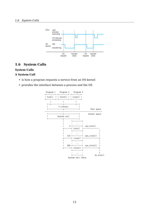
1.6 System Calls
System Calls
A System Call
• is how a program requests a service from an OS kernel
• provides the interface between a process and the OS
14

15. 1.6 System Calls
Program 1 Program 2 Program 3
+---------+ +---------+ +---------+
| fork() | | vfork() | | clone() |
+---------+ +---------+ +---------+
| | |
+--v-----------v-----------v--+
| C Library |
+--------------o--------------+ User space
-----------------|------------------------------------
+--------------v--------------+ Kernel space
| System call |
+--------------o--------------+
| +---------+
| : ... :
| 3 +---------+ sys_fork()
o------>| fork() |---------------.
| +---------+ |
| : ... : |
| 120 +---------+ sys_clone() |
o------>| clone() |---------------o
| +---------+ |
| : ... : |
| 289 +---------+ sys_vfork() |
o------>| vfork() |---------------o
+---------+ |
: ... : v
+---------+ do_fork()
System Call Table
User program 2
User program 1
Kernel call
Service
procedure
Dispatch table
User programs
run in
user mode
Operating
system
runs in
kernel mode
4
3
1
2
Mainmemory
Figure 1-16. How a system call can be made: (1) User pro-
gram traps to the kernel. (2) Operating system determines ser-
vice number required. (3) Operating system calls service pro-
cedure. (4) Control is returned to user program.
The 11 steps in making the system call read(fd,buffer,nbytes)
15

16. 1.6 System Calls
Return to caller
4
10
6
0
9
7 8
3
2
1
11
Dispatch
Sys call
handler
Address
0xFFFFFFFF
User space
Kernel space
(Operating system)
Library
procedure
read
User program
calling read
Trap to the kernel
Put code for read in register
Increment SP
Call read
Push fd
Push buffer
Push nbytes
5
Fig. 1-17. The 11 steps in making the system call
read(fd, buffer, nbytes).
Process management
Call Description
pid = fork( ) Create a child process identical to the parent
pid = waitpid(pid, statloc, options) Wait for a child to terminate
s = execve(name, argv, environp) Replace a process’ core image
exit(status) Terminate process execution and return status
File management
Call Description
fd = open(file, how, ...) Open a file for reading, writing or both
s = close(fd) Close an open file
n = read(fd, buffer, nbytes) Read data from a file into a buffer
n = write(fd, buffer, nbytes) Write data from a buffer into a file
position = lseek(fd, offset, whence) Move the file pointer
s = stat(name, buf) Get a file’s status information
Directory and file system management
Call Description
s = mkdir(name, mode) Create a new directory
s = rmdir(name) Remove an empty directory
s = link(name1, name2) Create a new entry, name2, pointing to name1
s = unlink(name) Remove a directory entry
s = mount(special, name, flag) Mount a file system
s = umount(special) Unmount a file system
Miscellaneous
Call Description
s = chdir(dirname) Change the working directory
s = chmod(name, mode) Change a file’s protection bits
s = kill(pid, signal) Send a signal to a process
seconds = time(seconds) Get the elapsed time since Jan. 1, 1970
Fig. 1-18. Some of the major POSIX system calls. The return code
s is −1 if an error has occurred. The return codes are as follows:
pid is a process id, fd is a file descriptor, n is a byte count, position
is an offset within the file, and seconds is the elapsed time. The
parameters are explained in the text.
System Call Examples
fork()
16

17. 1.6 System Calls
1 #include stdio.h
2 #include unistd.h
3
4 int main ()
5 {
6 printf(Hello World!n);
7 fork();
8 printf(Goodbye Cruel World!n);
9 return 0;
10 }
$ man 2 fork
exec()
1 #include stdio.h
2 #include unistd.h
3
4 int main ()
5 {
6 printf(Hello World!n);
7 if(fork() != 0 )
8 printf(I am the parent process.n);
9 else {
10 printf(A child is listing the directory contents...n);
11 execl(/bin/ls, ls, -al, NULL);
12 }
13 return 0;
14 }
$ man 3 exec
Hardware INT vs. Software INT
Device:
Send electrical signal to interrupt controller.
Controller:
1. Interrupt CPU.
2. Send digital identification of interrupting
device.
Kernel:
1. Save registers.
2. Execute driver software to read I/O device.
3. Send message.
4. Restart a process (not necessarily
interrupted process).
Caller:
1. Put message pointer and destination of
message into CPU registers.
2. Execute software interrupt instruction.
Kernel:
1. Save registers.
2. Send and/or receive message.
3. Restart a process (not necessarily calling
process).
(a) (b)
Figure 2-34. (a) How a hardware interrupt is processed. (b)
How a system call is made.
17

18. References
[1] Wikipedia. Interrupt — Wikipedia, The Free Encyclopedia. [Online; accessed 21-
February-2015]. 2015.
[2] Wikipedia. System call — Wikipedia, The Free Encyclopedia. [Online; accessed 21-
February-2015]. 2015.
2 Process And Thread
2.1 Processes
2.1.1 What’s a Process
Process
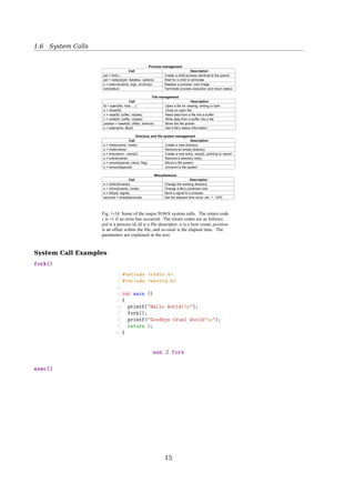
A process is an instance of a program in execution
Processes are like human beings:
« they are generated
« they have a life
« they optionally generate one or more child processes,
and
« eventually they die
A small difference:
• sex is not really common among processes
• each process has just one parent
Stack
Gap
Data
Text
0000
FFFF
The term ”process” is often used with several different meanings. In this book, we stick
to the usual OS textbook definition: a process is an instance of a program in execution.
You might think of it as the collection of data structures that fully describes how far the
execution of the program has progressed[2, Sec. 3.1, Processes, Lightweight Processes,
and Threads].
Processes are like human beings: they are generated, they have a more or less signifi-
cant life, they optionally generate one or more child processes, and eventually they die. A
small difference is that sex is not really common among processes each process has just
one parent.
From the kernel’s point of view, the purpose of a process is to act as an entity to which
system resources (CPU time, memory, etc.) are allocated.
In general, a computer system process consists of (or is said to ’own’) the following
resources[34]:
• An image of the executable machine code associated with a program.
• Memory (typically some region of virtual memory); which includes the executable
code, process-specific data (input and output), a call stack (to keep track of active
subroutines and/or other events), and a heap to hold intermediate computation data
generated during run time.
18

19. 2.1 Processes
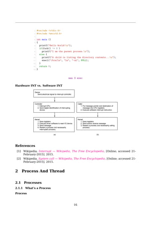
• Operating system descriptors of resources that are allocated to the process, such as
file descriptors (Unix terminology) or handles (Windows), and data sources and sinks.
• Security attributes, such as the process owner and the process’ set of permissions
(allowable operations).
• Processor state (context), such as the content of registers, physical memory address-
ing, etc. The state is typically stored in computer registers when the process is exe-
cuting, and in memory otherwise.
The operating system holds most of this information about active processes in data struc-
tures called process control blocks.
Any subset of resource, but typically at least the processor state, may be associated
with each of the process’ threads in operating systems that support threads or ’daughter’
processes.
The operating system keeps its processes separated and allocates the resources they
need, so that they are less likely to interfere with each other and cause system failures
(e.g., deadlock or thrashing). The operating system may also provide mechanisms for
inter-process communication to enable processes to interact in safe and predictable ways.
2.1.2 PCB
Process Control Block (PCB)
Implementation
A process is the collection of data structures that fully describes
how far the execution of the program has progressed.
• Each process is represented by a PCB
• task_struct in
+-------------------+
| process state |
+-------------------+
| PID |
+-------------------+
| program counter |
+-------------------+
| registers |
+-------------------+
| memory limits |
+-------------------+
| list of open files|
+-------------------+
| ... |
+-------------------+
To manage processes, the kernel must have a clear picture of what each process is
doing. It must know, for instance, the process’s priority, whether it is running on a CPU or
blocked on an event, what address space has been assigned to it, which files it is allowed to
address, and so on. This is the role of the process descriptor a task_struct type structure
whose fields contain all the information related to a single process. As the repository of so
much information, the process descriptor is rather complex. In addition to a large number
of fields containing process attributes, the process descriptor contains several pointers to
other data structures that, in turn, contain pointers to other structures[2, Sec. 3.2, Process
Descriptor].
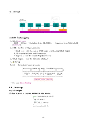
2.1.3 Process Creation
Process Creation
19

20. 2.1 Processes
exit()exec()
fork() wait()
anything()
parent
child
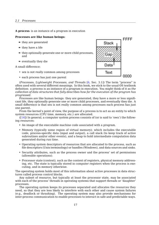
• When a process is created, it is almost identical to its parent
– It receives a (logical) copy of the parent’s address space, and
– executes the same code as the parent
• The parent and child have separate copies of the data (stack and heap)
When a process is created, it is almost identical to its parent. It receives a (logical) copy
of the parent’s address space and executes the same code as the parent, beginning at the
next instruction following the process creation system call. Although the parent and child
may share the pages containing the program code (text), they have separate copies of the
data (stack and heap), so that changes by the child to a memory location are invisible to
the parent (and vice versa) [2, Sec. 3.1, Processes, Lightweight Processes, and Threads].
While earlier Unix kernels employed this simple model, modern Unix systems do not.
They support multi-threaded applications user programs having many relatively indepen-
dent execution flows sharing a large portion of the application data structures. In such
systems, a process is composed of several user threads (or simply threads), each of which
represents an execution flow of the process. Nowadays, most multi-threaded applications
are written using standard sets of library functions called pthread (POSIX thread) libraries.
Traditional Unix systems treat all processes in the same way: resources owned by
the parent process are duplicated in the child process. This approach makes process
creation very slow and inefficient, because it requires copying the entire address space
of the parent process. The child process rarely needs to read or modify all the resources
inherited from the parent; in many cases, it issues an immediate execve() and wipes out
the address space that was so carefully copied [2, Sec. 3.4, Creating Processes].
Modern Unix kernels solve this problem by introducing three different mechanisms:
• Copy On Write
• Lightweight processes
• The vfork() system call
Forking in C
1 #include stdio.h
2 #include unistd.h
3
4 int main ()
5 {
6 printf(Hello World!n);
7 fork();
8 printf(Goodbye Cruel World!n);
9 return 0;
10 }
20

21. 2.1 Processes
$ man fork
exec()
1 int main()
2 {
3 pid_t pid;
4 /* fork another process */
5 pid = fork();
6 if (pid 0) { /* error occurred */
7 fprintf(stderr, Fork Failed);
8 exit(-1);
9 }
10 else if (pid == 0) { /* child process */
11 execlp(/bin/ls, ls, NULL);
12 }
13 else { /* parent process */
14 /* wait for the child to complete */
15 wait(NULL);
16 printf (Child Complete);
17 exit(0);
18 }
19 return 0;
20 }
$ man 3 exec
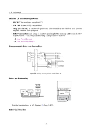
2.1.4 Process State
Process State Transition
1 23
4
Blocked
Running
Ready
1. Process blocks for input
2. Scheduler picks another process
3. Scheduler picks this process
4. Input becomes available
Fig. 2-2. A process can be in running, blocked, or ready state.
Transitions between these states are as shown.
See also [2, Sec. 3.2.1, Process State].
2.1.5 CPU Switch From Process To Process
CPU Switch From Process To Process
21

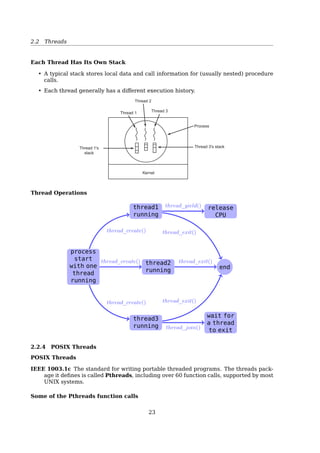
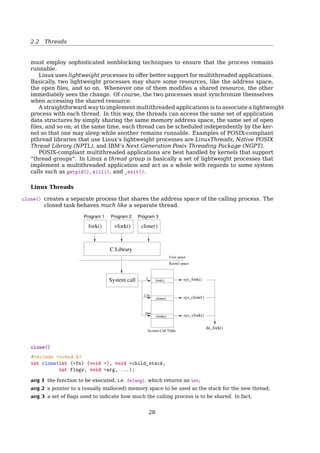
22. 2.2 Threads
See also: [2, Sec. 3.3, Process Switch].
2.2 Threads
2.2.1 Processes vs. Threads
Process vs. Thread
a single-threaded process = resource + execution
a multi-threaded process = resource + executions
Thread Thread
Kernel Kernel
Process 1 Process 1 Process 1 Process
User
space
Kernel
space
(a) (b)
Fig. 2-6. (a) Three processes each with one thread. (b) One process
with three threads.
A process = a unit of resource ownership, used to group resources together;
A thread = a unit of scheduling, scheduled for execution on the CPU.
Process vs. Thread
multiple threads running in one pro-
cess:
multiple processes running in one
computer:
share an address space and other re-
sources
share physical memory, disk, printers ...
No protection between threads
impossible — because process is the minimum unit of resource management
unnecessary — a process is owned by a single user
22

23. 2.2 Threads
Threads
+------------------------------------+
| code, data, open files, signals... |
+-----------+-----------+------------+
| thread ID | thread ID | thread ID |
+-----------+-----------+------------+
| program | program | program |
| counter | counter | counter |
+-----------+-----------+------------+
| register | register | register |
| set | set | set |
+-----------+-----------+------------+
| stack | stack | stack |
+-----------+-----------+------------+
2.2.2 Why Thread?
A Multi-threaded Web Server
Dispatcher thread
Worker thread
Web page cache
Kernel
Network
connection
Web server process
User
space
Kernel
space
Fig. 2-10. A multithreaded Web server.
while (TRUE) { while (TRUE) {
get next request(buf); wait for work(buf)
handoff work(buf); look for page in cache(buf, page);
} if (page not in cache(page))
read page from disk(buf, page);
return page(page);
}
(a) (b)
Fig. 2-11. A rough outline of the code for Fig. 2-10. (a) Dispatcher
thread. (b) Worker thread.
A Word Processor With 3 Threads
Kernel
Keyboard Disk
Four score and seven
years ago, our fathers
brought forth upon this
continent a new nation:
conceived in liberty,
and dedicated to the
proposition that all
men are created equal.
Now we are engaged
in a great civil war
testing whether that
nation, or any nation
so conceived and so
dedicated, can long
endure. We are met on
a great battlefield of
that war.
We have come to
dedicate a portion of
that field as a final
resting place for those
who here gave their
lives that this nation
might live. It is
altogether fitting and
proper that we should
do this.
But, in a larger sense,
we cannot dedicate, we
cannot consecrate we
cannot hallow this
ground. The brave
men, living and dead,
who struggled here
have consecrated it, far
above our poor power
to add or detract. The
world will little note,
nor long remember,
what we say here, but
it can never forget
what they did here.
It is for us the living,
rather, to be dedicated
here to the unfinished
work which they who
fought here have thus
far so nobly advanced.
It is rather for us to be
here dedicated to the
great task remaining
before us, that from
these honored dead we
take increased devotion
to that cause for which
they gave the last full
measure of devotion,
that we here highly
resolve that these dead
shall not have died in
vain that this nation,
under God, shall have
a new birth of freedom
and that government of
the people by the
people, for the people
Fig. 2-9. A word processor with three threads.23

24. 2.2 Threads
• Responsiveness
– Good for interactive applications.
– A process with multiple threads makes a great server (e.g. a web server):
Have one server process, many ”worker” threads – if one thread blocks (e.g.
on a read), others can still continue executing
• Economy – Threads are cheap!
– Cheap to create – only need a stack and storage for registers
– Use very little resources – don’t need new address space, global data, program
code, or OS resources
– switches are fast – only have to save/restore PC, SP, and registers
• Resource sharing – Threads can pass data via shared memory; no need for IPC
• Can take advantage of multiprocessors
2.2.3 Thread Characteristics
Thread States Transition
Same as process states transition
1 23
4
Blocked
Running
Ready
1. Process blocks for input
2. Scheduler picks another process
3. Scheduler picks this process
4. Input becomes available
Fig. 2-2. A process can be in running, blocked, or ready state.
Transitions between these states are as shown.
Each Thread Has Its Own Stack
• A typical stack stores local data and call information for (usually nested) procedure
calls.
• Each thread generally has a different execution history.
Kernel
Thread 3's stack
Process
Thread 3Thread 1
Thread 2
Thread 1's
stack
Fig. 2-8. Each thread has its own stack.
24

25. 2.2 Threads
Thread Operations
Start
with one
thread
running
thread1
thread2
thread3
end
release
CPU
wait for
a thread
to exit
thread_create()
thread_create()
thread_create()
thread_exit()
thread_yield()
thread_exit()
thread_exit()
thread_join()
2.2.4 POSIX Threads
POSIX Threads
IEEE 1003.1c The standard for writing portable threaded programs. The threads pack-
age it defines is called Pthreads, including over 60 function calls, supported by most
UNIX systems.
Some of the Pthreads function calls
Thread call Description
pthread_create Create a new thread
pthread_exit Terminate the calling thread
pthread_join Wait for a specific thread to exit
pthread_yield Release the CPU to let another thread run
pthread_attr_init Create and initialize a thread’s attribute structure
pthread_attr_destroy Remove a thread’s attribute structure
Pthreads
Example 1
25

26. 2.2 Threads
1 #include pthread.h
2 #include stdlib.h
3 #include unistd.h
4 #include stdio.h
5
6 void *thread_function(void *arg){
7 int i;
8 for( i=0; i20; i++ ){
9 printf(Thread says hi!n);
10 sleep(1);
11 }
12 return NULL;
13 }
14
15 int main(void){
16 pthread_t mythread;
17 if(pthread_create(mythread, NULL, thread_function, NULL)){
18 printf(error creating thread.);
19 abort();
20 }
21
22 if(pthread_join(mythread, NULL)){
23 printf(error joining thread.);
24 abort();
25 }
26 exit(0);
27 }
See also:
• IBM Developworks: POSIX threads explained3
• stackoverflow.com: What is the difference between exit() and abort()?4
Pthreads
pthread_t defined in pthread.h, is often called a ”thread id” (tid);
pthread_create() returns zero on success and a non-zero value on failure;
pthread_join() returns zero on success and a non-zero value on failure;
How to use pthread?
1. #includepthread.h
2. $ gcc thread1.c -o thread1 -pthread
3. $ ./thread1
3http://www.ibm.com/developerworks/linux/library/l-posix1/index.html
4http://stackoverflow.com/questions/397075/what-is-the-difference-between-exit-and-abort
26

27. 2.2 Threads
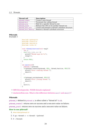
Pthreads
Example 2
1 #include pthread.h
2 #include stdio.h
3 #include stdlib.h
4
5 #define NUMBER_OF_THREADS 10
6
7 void *print_hello_world(void *tid)
8 {
9 /* prints the thread’s identifier, then exits.*/
10 printf (Thread %d: Hello World!n, tid);
11 pthread_exit(NULL);
12 }
13
14 int main(int argc, char *argv[])
15 {
16 pthread_t threads[NUMBER_OF_THREADS];
17 int status, i;
18 for (i=0; iNUMBER_OF_THREADS; i++)
19 {
20 printf (Main: creating thread %dn,i);
21 status = pthread_create(threads[i], NULL, print_hello_world, (void *)i);
22
23 if(status != 0){
24 printf (Oops. pthread_create returned error code %dn,status);
25 exit(-1);
26 }
27 }
28 exit(NULL);
29 }
Pthreads
With or without pthread_join()? Check it by yourself.
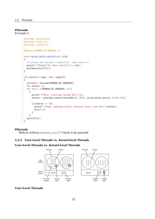
2.2.5 User-Level Threads vs. Kernel-level Threads
User-Level Threads vs. Kernel-Level Threads
Process ProcessThread Thread
Process
table
Process
table
Thread
table
Thread
table
Run-time
system
Kernel
space
User
space
KernelKernel
Fig. 2-13. (a) A user-level threads package. (b) A threads package
managed by the kernel.
User-Level Threads
27

28. 2.2 Threads
User-level threads provide a library of functions to allow user processes to create and
manage their own threads.
No need to modify the OS;
Simple representation
– each thread is represented simply by a PC, regs, stack, and a small TCB, all stored
in the user process’ address space
Simple Management
– creating a new thread, switching between threads, and synchronization between
threads can all be done without intervention of the kernel
Fast
– thread switching is not much more expensive than a procedure call
Flexible
– CPU scheduling (among threads) can be customized to suit the needs of the al-
gorithm – each process can use a different thread scheduling algorithm
User-Level Threads
Lack of coordination between threads and OS kernel
– Process as a whole gets one time slice
– Same time slice, whether process has 1 thread or 1000 threads
– Also – up to each thread to relinquish control to other threads in that process
Requires non-blocking system calls (i.e. a multithreaded kernel)
– Otherwise, entire process will blocked in the kernel, even if there are runnable
threads left in the process
– part of motivation for user-level threads was not to have to modify the OS
If one thread causes a page fault(interrupt!), the entire process blocks
See also: More about blocking and non-blocking calls5
Kernel-Level Threads
Kernel-level threads kernel provides system calls to create and manage threads
Kernel has full knowledge of all threads
– Scheduler may choose to give a process with 10 threads more time than process
with only 1 thread
Good for applications that frequently block (e.g. server processes with frequent in-
terprocess communication)
Slow – thread operations are 100s of times slower than for user-level threads
Significant overhead and increased kernel complexity – kernel must manage and
schedule threads as well as processes
– Requires a full thread control block (TCB) for each thread
5http://www.daniweb.com/software-development/computer-science/threads/384575/synchronous-vs-asynchronous-blocking-vs-non-blo
28

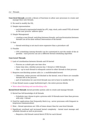
29. 2.2 Threads
Hybrid Implementations
Combine the advantages of two
Multiple user threads
on a kernel thread
User
space
Kernel
spaceKernel threadKernel
Fig. 2-14. Multiplexing user-level threads onto kernel-level
threads.
Programming Complications
• fork(): shall the child has the threads that its parent has?
• What happens if one thread closes a file while another is still reading from it?
• What happens if several threads notice that there is too little memory?
And sometimes, threads fix the symptom, but not the problem.
2.2.6 Linux Threads
Linux Threads
To the Linux kernel, there is no concept of a thread
• Linux implements all threads as standard processes
• To Linux, a thread is merely a process that shares certain resources with other pro-
cesses
• Some OS (MS Windows, Sun Solaris) have cheap threads and expensive processes.
• Linux processes are already quite lightweight
On a 75MHz Pentium
thread: 1.7µs
fork: 1.8µs
[2, Sec. 3.1, Processes, Lightweight Processes, and Threads] Older versions of the Linux
kernel offered no support for multithreaded applications. From the kernel point of view,
a multithreaded application was just a normal process. The multiple execution flows of a
multithreaded application were created, handled, and scheduled entirely in User Mode,
usually by means of a POSIX-compliant pthread library.
However, such an implementation of multithreaded applications is not very satisfac-
tory. For instance, suppose a chess program uses two threads: one of them controls the
graphical chessboard, waiting for the moves of the human player and showing the moves
of the computer, while the other thread ponders the next move of the game. While the
first thread waits for the human move, the second thread should run continuously, thus
exploiting the thinking time of the human player. However, if the chess program is just
a single process, the first thread cannot simply issue a blocking system call waiting for
29

30. 2.2 Threads
a user action; otherwise, the second thread is blocked as well. Instead, the first thread
must employ sophisticated nonblocking techniques to ensure that the process remains
runnable.
Linux uses lightweight processes to offer better support for multithreaded applications.
Basically, two lightweight processes may share some resources, like the address space,
the open files, and so on. Whenever one of them modifies a shared resource, the other
immediately sees the change. Of course, the two processes must synchronize themselves
when accessing the shared resource.
A straightforward way to implement multithreaded applications is to associate a light-
weight process with each thread. In this way, the threads can access the same set of
application data structures by simply sharing the same memory address space, the same
set of open files, and so on; at the same time, each thread can be scheduled independently
by the kernel so that one may sleep while another remains runnable. Examples of POSIX-
compliant pthread libraries that use Linux’s lightweight processes are LinuxThreads, Na-
tive POSIX Thread Library (NPTL), and IBM’s Next Generation Posix Threading Package
(NGPT).
POSIX-compliant multithreaded applications are best handled by kernels that support
”thread groups”. In Linux a thread group is basically a set of lightweight processes that
implement a multithreaded application and act as a whole with regards to some system
calls such as getpid(), kill(), and _exit().
Linux Threads
clone() creates a separate process that shares the address space of the calling process. The
cloned task behaves much like a separate thread.
Program 3
Kernel space
User space
fork()
clone()
vfork()
System Call Table
3
120
289
Program 1 Program 2
C Library
vfork()fork() clone()
System call sys_fork()
sys_clone()
sys_vfork()
do_fork()
clone()
1 #include sched.h
2 int clone(int (*fn) (void *), void *child_stack,
3 int flags, void *arg, ...);
arg 1 the function to be executed, i.e. fn(arg), which returns an int;
30

31. 2.2 Threads
arg 2 a pointer to a (usually malloced) memory space to be used as the stack for the new thread;
arg 3 a set of flags used to indicate how much the calling process is to be shared. In fact,
clone(0) == fork()
arg 4 the arguments passed to the function.
It returns the PID of the child process or -1 on failure.
$ man clone
The clone() System Call
Some flags:
flag Shared
CLONE_FS File-system info
CLONE_VM Same memory space
CLONE_SIGHAND Signal handlers
CLONE_FILES The set of open files
In practice, one should try to avoid calling clone() directly
Instead, use a threading library (such as pthreads) which use clone() when starting
a thread (such as during a call to pthread_create())
clone() Example
31

32. 1 #include unistd.h
2 #include sched.h
3 #include sys/types.h
4 #include stdlib.h
5 #include string.h
6 #include stdio.h
7 #include fcntl.h
8
9 int variable;
10
11 int do_something()
12 {
13 variable = 42;
14 _exit(0);
15 }
16
17 int main(void)
18 {
19 void *child_stack;
20 variable = 9;
21
22 child_stack = (void *) malloc(16384);
23 printf(The variable was %dn, variable);
24
25 clone(do_something, child_stack,
26 CLONE_FS | CLONE_VM | CLONE_FILES, NULL);
27 sleep(1);
28
29 printf(The variable is now %dn, variable);
30 return 0;
31 }
Stack Grows Downwards
child_stack = (void**)malloc(8192) + 8192/sizeof(*child_stack);
References
[1] Wikipedia. Process (computing) — Wikipedia, The Free Encyclopedia. [Online; ac-
cessed 21-February-2015]. 2014.
[2] Wikipedia. Process control block — Wikipedia, The Free Encyclopedia. [Online; ac-
cessed 21-February-2015]. 2015.
[3] Wikipedia. Thread (computing) — Wikipedia, The Free Encyclopedia. [Online; ac-
cessed 21-February-2015]. 2015.
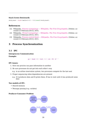
3 Process Synchronization
32

33. 3.1 IPC
3.1 IPC
Interprocess Communication
Example:
ps | head -2 | tail -1 | cut -f2 -d' '
IPC issues:
1. How one process can pass information to another
2. Be sure processes do not get into each other’s way
e.g. in an airline reservation system, two processes compete for the last seat
3. Proper sequencing when dependencies are present
e.g. if A produces data and B prints them, B has to wait until A has produced some
data
Two models of IPC:
• Shared memory
• Message passing (e.g. sockets)
Producer-Consumer Problem
compiler Assembly
code assembler
Object
module loader
Process
wants
printing
file
Printer
daemon
3.2 Shared Memory
Process Synchronization
Producer-Consumer Problem
• Consumers don’t try to remove objects from Buffer when it is empty.
• Producers don’t try to add objects to the Buffer when it is full.
Producer
1 while(TRUE){
2 while(FULL);
3 item = produceItem();
4 insertItem(item);
5 }
Consumer
1 while(TRUE){
2 while(EMPTY);
3 item = removeItem();
4 consumeItem(item);
5 }
How to define full/empty?
33

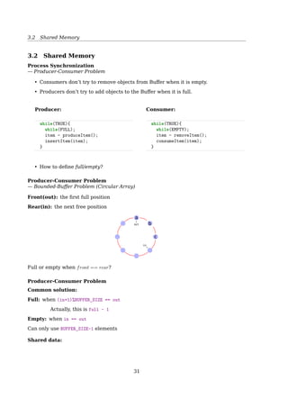
34. 3.2 Shared Memory
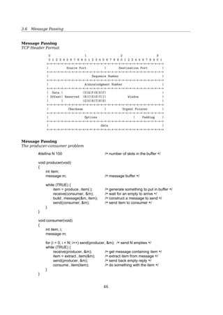
Producer-Consumer Problem
— Bounded-Buffer Problem (Circular Array)
Front(out): the first full position
Rear(in): the next free position
out
in
c
b
a
Full or empty when front == rear?
Producer-Consumer Problem
Common solution:
Full: when (in+1)%BUFFER_SIZE == out
Actually, this is full - 1
Empty: when in == out
Can only use BUFFER_SIZE-1 elements
Shared data:
1 #define BUFFER_SIZE 6
2 typedef struct {
3 ...
4 } item;
5 item buffer[BUFFER_SIZE];
6 int in = 0; //the next free position
7 int out = 0;//the first full position
Bounded-Buffer Problem
34

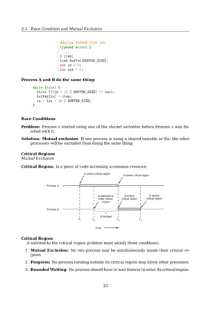
35. 3.3 Race Condition and Mutual Exclusion
Producer:
1 while (true) {
2 /* do nothing -- no free buffers */
3 while (((in + 1) % BUFFER_SIZE) == out);
4
5 buffer[in] = item;
6 in = (in + 1) % BUFFER_SIZE;
7 }
Consumer:
1 while (true) {
2 while (in == out); // do nothing
3 // remove an item from the buffer
4 item = buffer[out];
5 out = (out + 1) % BUFFER_SIZE;
6 return item;
7 }
out
in
c
b
a
3.3 Race Condition and Mutual Exclusion
Race Conditions
Now, let’s have two producers
4
5
6
7
abc
prog.c
prog.n
Process A
out = 4
in = 7
Process B
Spooler
directory
Fig. 2-18. Two processes want to access shared memory at the
same time.Race Conditions
Two producers
1 #define BUFFER_SIZE 100
2 typedef struct {
3 ...
4 } item;
5 item buffer[BUFFER_SIZE];
6 int in = 0;
7 int out = 0;
35

36. 3.3 Race Condition and Mutual Exclusion
Process A and B do the same thing:
1 while (true) {
2 while (((in + 1) % BUFFER_SIZE) == out);
3 buffer[in] = item;
4 in = (in + 1) % BUFFER_SIZE;
5 }
Race Conditions
Problem: Process B started using one of the shared variables before Process A was fin-
ished with it.
Solution: Mutual exclusion. If one process is using a shared variable or file, the other
processes will be excluded from doing the same thing.
Critical Regions
Mutual Exclusion
Critical Region: is a piece of code accessing a common resource.
A enters critical region
A leaves critical region
B attempts to
enter critical
region
B enters
critical region
T1
T2
T3
T4
Process A
Process B
B blocked
B leaves
critical region
Time
Fig. 2-19. Mutual exclusion using critical regions.
Critical Region
A solution to the critical region problem must satisfy three conditions:
Mutual Exclusion: No two process may be simultaneously inside their critical regions.
Progress: No process running outside its critical region may block other processes.
Bounded Waiting: No process should have to wait forever to enter its critical region.
Mutual Exclusion With Busy Waiting
Disabling Interrupts
1 {
2 ...
3 disableINT();
4 critical_code();
5 enableINT();
6 ...
7 }
36

37. 3.3 Race Condition and Mutual Exclusion
Problems:
• It’s not wise to give user process the power of turning off INTs.
– Suppose one did it, and never turned them on again
• useless for multiprocessor system
Disabling INTs is often a useful technique within the kernel itself but is not a general
mutual exclusion mechanism for user processes.
Mutual Exclusion With Busy Waiting
Lock Variables
1 int lock=0; //shared variable
2 {
3 ...
4 while(lock); //busy waiting
5 lock=1;
6 critical_code();
7 lock=0;
8 ...
9 }
Problem:
• What if an interrupt occurs right at line 5?
• Checking the lock again while backing from an interrupt?
Mutual Exclusion With Busy Waiting
Strict Alternation
Process 0
1 while(TRUE){
2 while(turn != 0);
3 critical_region();
4 turn = 1;
5 noncritical_region();
6 }
Process 1
1 while(TRUE){
2 while(turn != 1);
3 critical_region();
4 turn = 0;
5 noncritical_region();
6 }
Problem: violates condition-2
• One process can be blocked by another not in its critical region.
• Requires the two processes strictly alternate in entering their critical region.
Mutual Exclusion With Busy Waiting
Peterson’s Solution
int interest[0] = 0;
int interest[1] = 0;
int turn;
P0
1 interest[0] = 1;
2 turn = 1;
3 while(interest[1] == 1
4 turn == 1);
5 critical_section();
6 interest[0] = 0;
P1
1 interest[1] = 1;
2 turn = 0;
3 while(interest[0] == 1
4 turn == 0);
5 critical_section();
6 interest[1] = 0;
37

38. 3.3 Race Condition and Mutual Exclusion
References
[1] Wikipedia. Peterson’s algorithm — Wikipedia, The Free Encyclopedia. [Online; ac-
cessed 23-February-2015]. 2015.
Mutual Exclusion With Busy Waiting
Hardware Solution: The TSL Instruction
Lock the memory bus
enter region:
TSL REGISTER,LOCK | copy lock to register and set lock to 1
CMP REGISTER,#0 | was lock zero?
JNE enter region | if it was non zero, lock was set, so loop
RET | return to caller; critical region entered
leave region:
MOVE LOCK,#0 | store a 0 in lock
RET | return to caller
Fig. 2-22. Entering and leaving a critical region using the TSL
instruction.
See also: [19, Sec. 2.3.3, Mutual Exclusion With Busy Waiting, p. 124].
Mutual Exclusion Without Busy Waiting
Sleep Wakeup
1 #define N 100 /* number of slots in the buffer */
2 int count = 0; /* number of items in the buffer */
1 void producer(){
2 int item;
3 while(TRUE){
4 item = produce_item();
5 if(count == N)
6 sleep();
7 insert_item(item);
8 count++;
9 if(count == 1)
10 wakeup(consumer);
11 }
12 }
1 void consumer(){
2 int item;
3 while(TRUE){
4 if(count == 0)
5 sleep();
6 item = rm_item();
7 count--;
8 if(count == N - 1)
9 wakeup(producer);
10 consume_item(item);
11 }
12 }
Producer-Consumer Problem
Race Condition
Problem
1. Consumer is going to sleep upon seeing an empty buffer, but INT occurs;
2. Producer inserts an item, increasing count to 1, then call wakeup(consumer);
3. But the consumer is not asleep, though count was 0. So the wakeup() signal is lost;
4. Consumer is back from INT remembering count is 0, and goes to sleep;
5. Producer sooner or later will fill up the buffer and also goes to sleep;
6. Both will sleep forever, and waiting to be waken up by the other process. Deadlock!
38

39. 3.4 Semaphores
Producer-Consumer Problem
Race Condition
Solution: Add a wakeup waiting bit
1. The bit is set, when a wakeup is sent to an awaken process;
2. Later, when the process wants to sleep, it checks the bit first. Turns it off if it’s set,
and stays awake.
What if many processes try going to sleep?
3.4 Semaphores
What is a Semaphore?
• A locking mechanism
• An integer or ADT
that can only be operated with:
Atomic Operations
P() V()
Wait() Signal()
Down() Up()
Decrement() Increment()
... ...
1 down(S){
2 while(S=0);
3 S--;
4 }
1 up(S){
2 S++;
3 }
More meaningful names:
• increment_and_wake_a_waiting_process_if_any()
• decrement_and_block_if_the_result_is_negative()
Semaphore
How to ensure atomic?
1. For single CPU, implement up() and down() as system calls, with the OS disabling all
interrupts while accessing the semaphore;
2. For multiple CPUs, to make sure only one CPU at a time examines the semaphore, a
lock variable should be used with the TSL instructions.
Semaphore is a Special Integer
A semaphore is like an integer, with three differences:
1. You can initialize its value to any integer, but after that the only operations you are
allowed to perform are increment (S++) and decrement (S- -).
2. When a thread decrements the semaphore, if the result is negative (S ≤ 0), the thread
blocks itself and cannot continue until another thread increments the semaphore.
3. When a thread increments the semaphore, if there are other threads waiting, one of
the waiting threads gets unblocked.
39

40. 3.4 Semaphores
Why Semaphores?
We don’t need semaphores to solve synchronization problems, but there are some ad-
vantages to using them:
• Semaphores impose deliberate constraints that help programmers avoid errors.
• Solutions using semaphores are often clean and organized, making it easy to demon-
strate their correctness.
• Semaphores can be implemented efficiently on many systems, so solutions that use
semaphores are portable and usually efficient.
The Simplest Use of Semaphore
Signaling
• One thread sends a signal to another thread to indicate that something has happened
• it solves the serialization problem
Signaling makes it possible to guarantee that a section of code in one thread will
run before a section of code in another thread
Thread A
1 statement a1
2 sem.signal()
Thread B
1 sem.wait()
2 statement b1
What’s the initial value of sem?
Semaphore
Rendezvous Puzzle
Thread A
1 statement a1
2 statement a2
Thread B
1 statement b1
2 statement b2
Q: How to guarantee that
1. a1 happens before b2, and
2. b1 happens before a2
a1 → b2; b1 → a2
Hint: Use two semaphores initialized to 0.
40

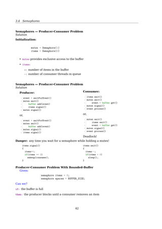
41. 3.4 Semaphores
Thread A: Thread B:
Solution 1:
statement a1 statement b1
sem1.wait() sem1.signal()
sem2.signal() sem2.wait()
statement a2 statement b2
Solution 2:
statement a1 statement b1
sem2.signal() sem1.signal()
sem1.wait() sem2.wait()
statement a2 statement b2
Solution 3:
statement a1 statement b1
sem2.wait() sem1.wait()
sem1.signal() sem2.signal()
statement a2 statement b2
Solution 3 has deadlock!
Mutex
• A second common use for semaphores is to enforce mutual exclusion
• It guarantees that only one thread accesses the shared variable at a time
• A mutex is like a token that passes from one thread to another, allowing one thread at
a time to proceed
Q: Add semaphores to the following example to enforce mutual exclusion to the shared
variable i.
Thread A: i++ Thread B: i++
Why? Because i++ is not atomic.
i++ is not atomic in assembly language
1 LOAD [i], r0 ;load the value of 'i' into
2 ;a register from memory
3 ADD r0, 1 ;increment the value
4 ;in the register
5 STORE r0, [i] ;write the updated
6 ;value back to memory
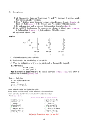
Interrupts might occur in between. So, i++ needs to be protected with a mutex.
Mutex Solution
Create a semaphore named mutex that is initialized to 1
1: a thread may proceed and access the shared variable
0: it has to wait for another thread to release the mutex
Thread A
1 mutex.wait()
2 i++
3 mutex.signal()
Thread B
1 mutex.wait()
2 i++
3 mutex.signal()
41

42. 3.4 Semaphores
Multiplex — Without Busy Waiting
1 typedef struct{
2 int space; //number of free resources
3 struct process *P; //a list of queueing producers
4 struct process *C; //a list of queueing consumers
5 } semaphore;
6 semaphore S;
7 S.space = 5;
Producer
1 void down(S){
2 S.space--;
3 if(S.space == 4){
4 rmFromQueue(S.C);
5 wakeup(S.C);
6 }
7 if(S.space 0){
8 addToQueue(S.P);
9 sleep();
10 }
11 }
Consumer
1 void up(S){
2 S.space++;
3 if(S.space 5){
4 addToQueue(S.C);
5 sleep();
6 }
7 if(S.space = 0){
8 rmFromQueue(S.P);
9 wakeup(S.P);
10 }
11 }
if S.space 0,
S.space == Number of queueing producers
if S.space 5,
S.space == Number of queueing consumers + 5
The work flow: There are several processes running simultaneously. They all need to
access some common resources.
1. Assuming S.space == 3 in the beginning
2. Process P1 comes and take one resource away. S.space == 2 now.
3. Process P2 comes and take the 2nd resource away. S.space == 1 now.
4. Process P3 comes and take the last resource away. S.space == 0 now.
5. Process P4 comes and sees nothing left. It has to sleep. S.space == -1 now.
6. Process P5 comes and sees nothing left. It has to sleep. S.space == -2 now.
7. At this moment, there are 2 processes (P4 and P5) sleeping. In another word,
they are queuing for resources.
8. Now, P1 finishes using the resource, and released it. After it does a S.space++, it
finds out that S.space = 0. So it wakes up a Process (say P4) in the queue.
9. P4 wakes up, and back to execute the instruction right after sleep().
10. P4 (or P2|P3) finishes using the resource, and releases it. After it does a S.space++,
it finds out that S.space = 0. So it wakes up P5 in the queue.
11. the queue is empty now.
Barrier
Barrier
Barrier
Barrier
A A A
B B B
C C
D D D
Time Time Time
Process
(a) (b) (c)
C
Fig. 2-30. Use of a barrier. (a) Processes approaching a barrier.
(b) All processes but one blocked at the barrier. (c) When the last
process arrives at the barrier, all of them are let through.
1. Processes approaching a barrier
42

43. 3.4 Semaphores
2. All processes but one blocked at the barrier
3. When the last process arrives at the barrier, all of them are let through
Synchronization requirement:
specific_task()
critical_point()
No thread executes critical_point() until after all threads have executed specific_task().
Barrier Solution
1 n = the number of threads
2 count = 0
3 mutex = Semaphore(1)
4 barrier = Semaphore(0)
count: keeps track of how many threads have arrived
mutex: provides exclusive access to count
barrier: is locked (≤ 0) until all threads arrive
When barrier.value0,
barrier.value == Number of queueing processes
Solution 1
1 specific_task();
2 mutex.wait();
3 count++;
4 mutex.signal();
5 if (count n)
6 barrier.wait();
7 barrier.signal();
8 critical_point();
Solution 2
1 specific_task();
2 mutex.wait();
3 count++;
4 mutex.signal();
5 if (count == n)
6 barrier.signal();
7 barrier.wait();
8 critical_point();
Only one thread can pass the barrier!
Barrier Solution
Solution 3
1 specific_task();
2
3 mutex.wait();
4 count++;
5 mutex.signal();
6
7 if (count == n)
8 barrier.signal();
9
10 barrier.wait();
11 barrier.signal();
12
13 critical_point();
Solution 4
1 specific_task();
2
3 mutex.wait();
4 count++;
5
6 if (count == n)
7 barrier.signal();
8
9 barrier.wait();
10 barrier.signal();
11 mutex.signal();
12
13 critical_point();
Blocking on a semaphore while holding a mutex!
barrier.wait();
barrier.signal();
43

44. 3.4 Semaphores
Turnstile
This pattern, a wait and a signal in rapid succession, occurs often enough that it has a
name called a turnstile, because
• it allows one thread to pass at a time, and
• it can be locked to bar all threads
Semaphores
Producer-Consumer Problem
Whenever an event occurs
• a producer thread creates an event object and adds it to the event buffer. Concur-
rently,
• consumer threads take events out of the buffer and process them. In this case, the
consumers are called “event handlers”.
Producer
1 event = waitForEvent()
2 buffer.add(event)
Consumer
1 event = buffer.get()
2 event.process()
Q: Add synchronization statements to the producer and consumer code to enforce the
synchronization constraints
1. Mutual exclusion
2. Serialization
See also [5, Sec. 4.1, Producer-Consumer Problem].
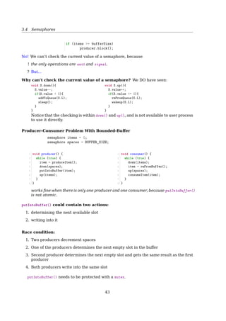
Semaphores — Producer-Consumer Problem
Solution
Initialization:
mutex = Semaphore(1)
items = Semaphore(0)
• mutex provides exclusive access to the buffer
• items:
+: number of items in the buffer
−: number of consumer threads in queue
44

45. 3.4 Semaphores
Semaphores — Producer-Consumer Problem
Solution
Producer
1 event = waitForEvent()
2 mutex.wait()
3 buffer.add(event)
4 items.signal()
5 mutex.signal()
or,
Producer
1 event = waitForEvent()
2 mutex.wait()
3 buffer.add(event)
4 mutex.signal()
5 items.signal()
Consumer
1 items.wait()
2 mutex.wait()
3 event = buffer.get()
4 mutex.signal()
5 event.process()
or,
Consumer
1 mutex.wait()
2 items.wait()
3 event = buffer.get()
4 mutex.signal()
5 event.process()
Danger: any time you wait for a semaphore while holding a mutex!
items.signal()
{
items++;
if(items == 0)
wakeup(consumer);
}
items.wait()
{
items--;
if(items 0)
sleep();
}
Producer-Consumer Problem With Bounded-Buffer
Given:
semaphore items = 0;
semaphore spaces = BUFFER_SIZE;
Can we?
if (items = BUFFER_SIZE)
producer.block();
if: the buffer is full
then: the producer blocks until a consumer removes an item
No! We can’t check the current value of a semaphore, because
! the only operations are wait and signal.
? But...
Why can’t check the current value of a semaphore? We DO have seen:
void S.down(){
S.value--;
if(S.value 0){
addToQueue(S.L);
sleep();
}
}
void S.up(){
S.value++;
if(S.value = 0){
rmFromQueue(S.L);
wakeup(S.L);
}
}
Notice that the checking is within down() and up(), and is not available to user process
to use it directly.
45

46. 3.4 Semaphores
Producer-Consumer Problem With Bounded-Buffer
1 semaphore items = 0;
2 semaphore spaces = BUFFER_SIZE;
1 void producer() {
2 while (true) {
3 item = produceItem();
4 down(spaces);
5 putIntoBuffer(item);
6 up(items);
7 }
8 }
1 void consumer() {
2 while (true) {
3 down(items);
4 item = rmFromBuffer();
5 up(spaces);
6 consumeItem(item);
7 }
8 }
works fine when there is only one producer and one consumer, because putIntoBuffer()
is not atomic.
putIntoBuffer() could contain two actions:
1. determining the next available slot
2. writing into it
Race condition:
1. Two producers decrement spaces
2. One of the producers determines the next empty slot in the buffer
3. Second producer determines the next empty slot and gets the same result as the first
producer
4. Both producers write into the same slot
putIntoBuffer() needs to be protected with a mutex.
With a mutex
1 semaphore mutex = 1; //controls access to c.r.
2 semaphore items = 0;
3 semaphore spaces = BUFFER_SIZE;
1 void producer() {
2 while (true) {
3 item = produceItem();
4 down(spaces);
5 down(mutex);
6 putIntoBuffer(item);
7 up(mutex);
8 up(items);
9 }
10 }
1 void consumer() {
2 while (true) {
3 down(items);
4 down(mutex);
5 item = rmFromBuffer();
6 up(mutex);
7 up(spaces);
8 consumeItem(item);
9 }
10 }
46

47. 3.5 Monitors
3.5 Monitors
Monitors
Monitor a high-level synchronization object for achieving mutual exclusion.
• It’s a language concept, and C does not have it.
• Only one process can be active in a monitor at
any instant.
• It is up to the compiler to implement mutual ex-
clusion on monitor entries.
– The programmer just needs to know that by
turning all the critical regions into monitor
procedures, no two processes will ever exe-
cute their critical regions at the same time.
1 monitor example
2 integer i;
3 condition c;
4
5 procedure producer();
6 ...
7 end;
8
9 procedure consumer();
10 ...
11 end;
12 end monitor;
Monitor
The producer-consumer problem
1 monitor ProducerConsumer
2 condition full, empty;
3 integer count;
4
5 procedure insert(item: integer);
6 begin
7 if count = N then wait(full);
8 insert_item(item);
9 count := count + 1;
10 if count = 1 then signal(empty)
11 end;
12
13 function remove: integer;
14 begin
15 if count = 0 then wait(empty);
16 remove = remove_item;
17 count := count - 1;
18 if count = N - 1 then signal(full)
19 end;
20 count := 0;
21 end monitor;
1 procedure producer;
2 begin
3 while true do
4 begin
5 item = produce_item;
6 ProducerConsumer.insert(item)
7 end
8 end;
9
10 procedure consumer;
11 begin
12 while true do
13 begin
14 item = ProducerConsumer.remove;
15 consume_item(item)
16 end
17 end;
3.6 Message Passing
Message Passing
• Semaphores are too low level
• Monitors are not usable except in a few programming languages
• Neither monitor nor semaphore is suitable for distributed systems
• No conflicts, easier to implement
Message passing uses two primitives, send and receive system calls:
- send(destination, message);
- receive(source, message);
47

48. 3.6 Message Passing
Message Passing
Design issues
• Message can be lost by network; — ACK
• What if the ACK is lost? — SEQ
• What if two processes have the same name? — socket
• Am I talking with the right guy? Or maybe a MIM? — authentication
• What if the sender and the receiver on the same machine? — Copying messages is
always slower than doing a semaphore operation or entering a monitor.
Message Passing
TCP Header Format
0 1 2 3
0 1 2 3 4 5 6 7 8 9 0 1 2 3 4 5 6 7 8 9 0 1 2 3 4 5 6 7 8 9 0 1
+-+-+-+-+-+-+-+-+-+-+-+-+-+-+-+-+-+-+-+-+-+-+-+-+-+-+-+-+-+-+-+-+
| Source Port | Destination Port |
+-+-+-+-+-+-+-+-+-+-+-+-+-+-+-+-+-+-+-+-+-+-+-+-+-+-+-+-+-+-+-+-+
| Sequence Number |
+-+-+-+-+-+-+-+-+-+-+-+-+-+-+-+-+-+-+-+-+-+-+-+-+-+-+-+-+-+-+-+-+
| Acknowledgment Number |
+-+-+-+-+-+-+-+-+-+-+-+-+-+-+-+-+-+-+-+-+-+-+-+-+-+-+-+-+-+-+-+-+
| Data | |U|A|P|R|S|F| |
| Offset| Reserved |R|C|S|S|Y|I| Window |
| | |G|K|H|T|N|N| |
+-+-+-+-+-+-+-+-+-+-+-+-+-+-+-+-+-+-+-+-+-+-+-+-+-+-+-+-+-+-+-+-+
| Checksum | Urgent Pointer |
+-+-+-+-+-+-+-+-+-+-+-+-+-+-+-+-+-+-+-+-+-+-+-+-+-+-+-+-+-+-+-+-+
| Options | Padding |
+-+-+-+-+-+-+-+-+-+-+-+-+-+-+-+-+-+-+-+-+-+-+-+-+-+-+-+-+-+-+-+-+
| data |
+-+-+-+-+-+-+-+-+-+-+-+-+-+-+-+-+-+-+-+-+-+-+-+-+-+-+-+-+-+-+-+-+
Message Passing
The producer-consumer problem
1 #define N 100 /* number of slots in the buffer */
2 void producer(void)
3 {
4 int item;
5 message m; /* message buffer */
6 while (TRUE) {
7 item = produce_item(); /* generate something to put in buffer */
8 receive(consumer, m); /* wait for an empty to arrive */
9 build_message(m, item); /* construct a message to send */
10 send(consumer, m); /* send item to consumer */
11 }
12 }
13
14 void consumer(void)
15 {
16 int item, i;
17 message m;
18 for (i=0; iN; i++) send(producer, m); /* send N empties */
19 while (TRUE) {
20 receive(producer, m); /* get message containing item */
21 item = extract_item(m); /* extract item from message */
22 send(producer, m); /* send back empty reply */
23 consume_item(item); /* do something with the item */
24 }
25 }
48

49. 3.7 Classical IPC Problems
3.7 Classical IPC Problems
3.7.1 The Dining Philosophers Problem
The Dining Philosophers Problem
1 while True:
2 think()
3 get_forks()
4 eat()
5 put_forks()
How to implement get_forks() and put_forks() to ensure
1. No deadlock
2. No starvation
3. Allow more than one philosopher to eat at the same time
The Dining Philosophers Problem
Deadlock
#define N 5 /* number of philosophers */
void philosopher(int i) /* i: philosopher number, from 0 to 4 */
{
while (TRUE) {
think( ); /* philosopher is thinking */
take fork(i); /* take left fork */
take fork((i+1) % N); /* take right fork; % is modulo operator */
eat( ); /* yum-yum, spaghetti */
put fork(i); /* put left fork back on the table */
put fork((i+1) % N); /* put right fork back on the table */
}
}
Fig. 2-32. A nonsolution to the dining philosophers problem.
• Put down the left fork and wait for a while if the right one is not available? Similar
to CSMA/CD — Starvation
The Dining Philosophers Problem
With One Mutex
1 #define N 5
2 semaphore mutex=1;
3
4 void philosopher(int i)
5 {
6 while (TRUE) {
7 think();
8 wait(mutex);
9 take_fork(i);
10 take_fork((i+1) % N);
11 eat();
12 put_fork(i);
13 put_fork((i+1) % N);
14 signal(mutex);
15 }
16 }
• Only one philosopher can eat at a time.
• How about 2 mutexes? 5 mutexes?
49

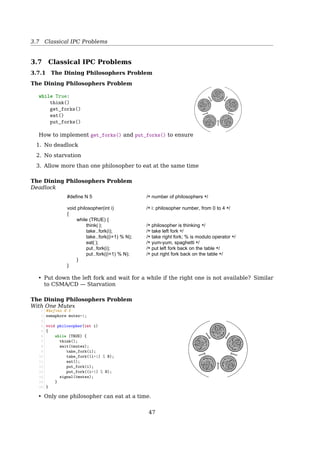
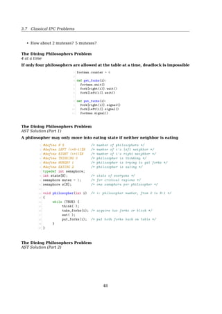
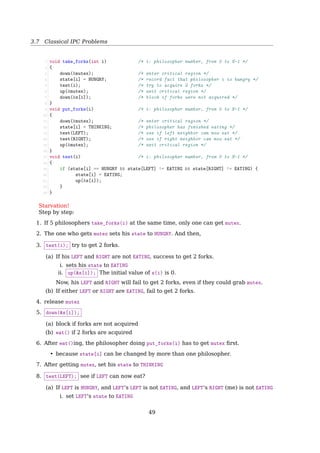
50. 3.7 Classical IPC Problems
The Dining Philosophers Problem
AST Solution (Part 1)
A philosopher may only move into eating state if neither neighbor is eating
1 #define N 5 /* number of philosophers */
2 #define LEFT (i+N-1)%N /* number of i’s left neighbor */
3 #define RIGHT (i+1)%N /* number of i’s right neighbor */
4 #define THINKING 0 /* philosopher is thinking */
5 #define HUNGRY 1 /* philosopher is trying to get forks */
6 #define EATING 2 /* philosopher is eating */
7 typedef int semaphore;
8 int state[N]; /* state of everyone */
9 semaphore mutex = 1; /* for critical regions */
10 semaphore s[N]; /* one semaphore per philosopher */
11
12 void philosopher(int i) /* i: philosopher number, from 0 to N-1 */
13 {
14 while (TRUE) {
15 think( );
16 take_forks(i); /* acquire two forks or block */
17 eat( );
18 put_forks(i); /* put both forks back on table */
19 }
20 }
The Dining Philosophers Problem
AST Solution (Part 2)
1 void take_forks(int i) /* i: philosopher number, from 0 to N-1 */
2 {
3 down(mutex); /* enter critical region */
4 state[i] = HUNGRY; /* record fact that philosopher i is hungry */
5 test(i); /* try to acquire 2 forks */
6 up(mutex); /* exit critical region */
7 down(s[i]); /* block if forks were not acquired */
8 }
9 void put_forks(i) /* i: philosopher number, from 0 to N-1 */
10 {
11 down(mutex); /* enter critical region */
12 state[i] = THINKING; /* philosopher has finished eating */
13 test(LEFT); /* see if left neighbor can now eat */
14 test(RIGHT); /* see if right neighbor can now eat */
15 up(mutex); /* exit critical region */
16 }
17 void test(i) /* i: philosopher number, from 0 to N-1 */
18 {
19 if (state[i] == HUNGRY state[LEFT] != EATING state[RIGHT] != EATING) {
20 state[i] = EATING;
21 up(s[i]);
22 }
23 }
Starvation!
Step by step:
50

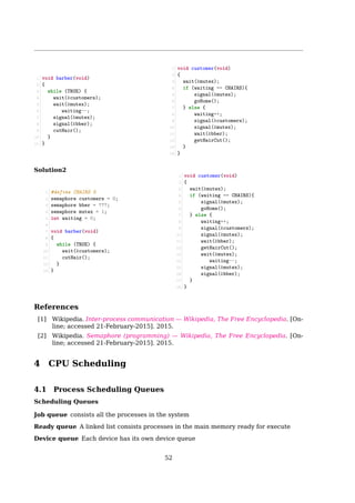
51. 3.7 Classical IPC Problems
1. If 5 philosophers take_forks(i) at the same time, only one can get mutex.
2. The one who gets mutex sets his state to HUNGRY. And then,
3. test(i); try to get 2 forks.
(a) If his LEFT and RIGHT are not EATING, success to get 2 forks.
i. sets his state to EATING
ii. up(s[i]); The initial value of s(i) is 0.
Now, his LEFT and RIGHT will fail to get 2 forks, even if they could grab mutex.
(b) If either LEFT or RIGHT are EATING, fail to get 2 forks.
4. release mutex
5. down(s[i]);
(a) block if forks are not acquired
(b) eat() if 2 forks are acquired
6. After eat()ing, the philosopher doing put_forks(i) has to get mutex first.
• because state[i] can be changed by more than one philosopher.
7. After getting mutex, set his state to THINKING
8. test(LEFT); see if LEFT can now eat?
(a) If LEFT is HUNGRY, and LEFT’s LEFT is not EATING, and LEFT’s RIGHT (me) is not EATING
i. set LEFT’s state to EATING
ii. up(s[LEFT]);
(b) If LEFT is not HUNGRY, or LEFT’s LEFT is EATING, or LEFT’s RIGHT (me) is EATING, LEFT
fails to get 2 forks.
9. test(RIGHT); see if RIGHT can now eat?
10. release mutex
The Dining Philosophers Problem
More Solutions
• If there is at least one leftie and at least one rightie, then deadlock is not possible
• Wikipedia: Dining philosophers problem
See also: [23, Dining philosophers problem]
51

52. 3.7 Classical IPC Problems
3.7.2 The Readers-Writers Problem
The Readers-Writers Problem
Constraint: no process may access the shared data for reading or writing while another
process is writing to it.
1 semaphore mutex = 1;
2 semaphore noOther = 1;
3 int readers = 0;
4
5 void writer(void)
6 {
7 while (TRUE) {
8 wait(noOther);
9 writing();
10 signal(noOther);
11 }
12 }
1 void reader(void)
2 {
3 while (TRUE) {
4 wait(mutex);
5 readers++;
6 if (readers == 1)
7 wait(noOther);
8 signal(mutex);
9 reading();
10 wait(mutex);
11 readers--;
12 if (readers == 0)
13 signal(noOther);
14 signal(mutex);
15 anything();
16 }
17 }
Starvation The writer could be blocked forever if there are always someone reading.
The Readers-Writers Problem
No starvation
1 semaphore mutex = 1;
2 semaphore noOther = 1;
3 semaphore turnstile = 1;
4 int readers = 0;
5
6 void writer(void)
7 {
8 while (TRUE) {
9 turnstile.wait();
10 wait(noOther);
11 writing();
12 signal(noOther);
13 turnstile.signal();
14 }
15 }
1 void reader(void)
2 {
3 while (TRUE) {
4 turnstile.wait();
5 turnstile.signal();
6
7 wait(mutex);
8 readers++;
9 if (readers == 1)
10 wait(noOther);
11 signal(mutex);
12 reading();
13 wait(mutex);
14 readers--;
15 if (readers == 0)
16 signal(noOther);
17 signal(mutex);
18 anything();
19 }
20 }
3.7.3 The Sleeping Barber Problem
The Sleeping Barber Problem
52

53. 3.7 Classical IPC Problems
Where’s the problem?
• the barber saw an empty room right before a customer arrives the waiting room;
• Several customer could race for a single chair;
Solution
1 #define CHAIRS 5
2 semaphore customers = 0; // any customers or not?
3 semaphore bber = 0; // barber is busy
4 semaphore mutex = 1;
5 int waiting = 0; // queueing customers
1 void barber(void)
2 {
3 while (TRUE) {
4 wait(customers);
5 wait(mutex);
6 waiting--;
7 signal(mutex);
8 signal(bber);
9 cutHair();
10 }
11 }
1 void customer(void)
2 {
3 wait(mutex);
4 if (waiting == CHAIRS){
5 signal(mutex);
6 goHome();
7 } else {
8 waiting++;
9 signal(customers);
10 signal(mutex);
11 wait(bber);
12 getHairCut();
13 }
14 }
Solution2
1 #define CHAIRS 5
2 semaphore customers = 0;
3 semaphore bber = ???;
4 semaphore mutex = 1;
5 int waiting = 0;
6
7 void barber(void)
8 {
9 while (TRUE) {
10 wait(customers);
11 cutHair();
12 }
13 }
1 void customer(void)
2 {
3 wait(mutex);
4 if (waiting == CHAIRS){
5 signal(mutex);
6 goHome();
7 } else {
8 waiting++;
9 signal(customers);
10 signal(mutex);
11 wait(bber);
12 getHairCut();
13 wait(mutex);
14 waiting--;
15 signal(mutex);
16 signal(bber);
17 }
18 }
53

54. References
[1] Wikipedia. Inter-process communication — Wikipedia, The Free Encyclopedia. [On-
line; accessed 21-February-2015]. 2015.
[2] Wikipedia. Semaphore (programming) — Wikipedia, The Free Encyclopedia. [On-
line; accessed 21-February-2015]. 2015.
4 CPU Scheduling
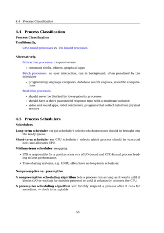
4.1 Process Scheduling Queues
Scheduling Queues
Job queue consists all the processes in the system
Ready queue A linked list consists processes in the main memory ready for execute
Device queue Each device has its own device queue3.2 Process Scheduling 105
queue header PCB7
PCB3
PCB5
PCB14 PCB6
PCB2
head
head
head
head
head
ready
queue
disk
unit 0
terminal
unit 0
mag
tape
unit 0
mag
tape
unit 1
tail registers registers
tail
tail
tail
tail
•
•
•
•
•
•
•
•
•
Figure 3.6 The ready queue and various I/O device queues.
The system also includes other queues. When a process is allocated the
CPU, it executes for a while and eventually quits, is interrupted, or waits for
the occurrence of a particular event, such as the completion of an I/O request.
Suppose the process makes an I/O request to a shared device, such as a disk.
Since there are many processes in the system, the disk may be busy with the
I/O request of some other process. The process therefore may have to wait for
the disk. The list of processes waiting for a particular I/O device is called a
device queue. Each device has its own device queue (Figure 3.6).
A common representation of process scheduling is a queueing diagram,
such as that in Figure 3.7. Each rectangular box represents a queue. Two types
of queues are present: the ready queue and a set of device queues. The circles
represent the resources that serve the queues, and the arrows indicate the flow
of processes in the system.
A new process is initially put in the ready queue. It waits there until it is
selected for execution, or is dispatched. Once the process is allocated the CPU
and is executing, one of several events could occur:
• The process could issue an I/O request and then be placed in an I/O queue.
• The process could create a new subprocess and wait for the subprocess’s
termination.
• The process could be removed forcibly from the CPU as a result of an
interrupt, and be put back in the ready queue.
• The tail pointer — When adding a new process to the queue, don’t have to find the
tail by traversing the list
Queueing Diagram
54

55. 4.2 Scheduling
106 Chapter 3 Processes
ready queue CPU
I/O I/O queue I/O request
time slice
expired
fork a
child
wait for an
interrupt
interrupt
occurs
child
executes
Figure 3.7 Queueing-diagram representation of process scheduling.
In the first two cases, the process eventually switches from the waiting state
to the ready state and is then put back in the ready queue. A process continues
this cycle until it terminates, at which time it is removed from all queues and
has its PCB and resources deallocated.
3.2.2 Schedulers
A process migrates among the various scheduling queues throughout its
lifetime. The operating system must select, for scheduling purposes, processes
from these queues in some fashion. The selection process is carried out by the
appropriate scheduler.
Often, in a batch system, more processes are submitted than can be executed
immediately. These processes are spooled to a mass-storage device (typically a
disk), where they are kept for later execution. The long-term scheduler, or job
scheduler, selects processes from this pool and loads them into memory for
execution. The short-term scheduler, or CPU scheduler, selects from among
the processes that are ready to execute and allocates the CPU to one of them.
The primary distinction between these two schedulers lies in frequency
of execution. The short-term scheduler must select a new process for the CPU
frequently. A process may execute for only a few milliseconds before waiting
for an I/O request. Often, the short-term scheduler executes at least once every
100 milliseconds. Because of the short time between executions, the short-term
scheduler must be fast. If it takes 10 milliseconds to decide to execute a process
for 100 milliseconds, then 10/(100 + 10) = 9 percent of the CPU is being used
(wasted) simply for scheduling the work.
The long-term scheduler executes much less frequently; minutes may sep-
arate the creation of one new process and the next. The long-term scheduler
controls the degree of multiprogramming (the number of processes in mem-
ory). If the degree of multiprogramming is stable, then the average rate of
process creation must be equal to the average departure rate of processes
4.2 Scheduling
Scheduling
• Scheduler uses scheduling algorithm to choose a process from the ready queue
• Scheduling doesn’t matter much on simple PCs, because
1. Most of the time there is only one active process
2. The CPU is too fast to be a scarce resource any more
• Scheduler has to make efficient use of the CPU because process switching is expen-
sive
1. User mode → kernel mode
2. Save process state, registers, memory map...
3. Selecting a new process to run by running the scheduling algorithm
4. Load the memory map of the new process
5. The process switch usually invalidates the entire memory cache
Scheduling Algorithm Goals
All systems
Fairness giving each process a fair share of the CPU
Policy enforcement seeing that stated policy is carried out
Balance keeping all parts of the system busy
Batch systems
Throughput maximize jobs per hour
Turnaround time minimize time between submission and termination
CPU utilization keep the CPU busy all the time
Interactive systems
55

56. 4.3 Process Behavior
Response time respond to requests quickly
Proportionality meet users’ expectations
Real-time systems
Meeting deadlines avoid losing data
Predictability avoid quality degradation in multimedia systems
See also: [19, Sec. 2.4.1.5, Scheduling Algorithm Goals, p. 150].
4.3 Process Behavior
Process Behavior
CPU-bound vs. I/O-bound
Types of CPU bursts:
• long bursts – CPU bound (i.e. batch work)
• short bursts – I/O bound (i.e. emacs)
Long CPU burst
Short CPU burst
Waiting for I/O
(a)
(b)
Time
Fig. 2-37. Bursts of CPU usage alternate with periods of waiting
for I/O. (a) A CPU-bound process. (b) An I/O-bound process.
As CPUs get faster, processes tend to get more I/O-bound.
4.4 Process Classification
Process Classification
Traditionally
CPU-bound processes vs. I/O-bound processes
Alternatively
Interactive processes responsiveness
• command shells, editors, graphical apps
Batch processes no user interaction, run in background, often penalized by the sched-
uler
• programming language compilers, database search engines, scientific computa-
tions
Real-time processes video and sound apps, robot controllers, programs that collect data
from physical sensors
56

57. 4.5 Process Schedulers
• should never be blocked by lower-priority processes
• should have a short guaranteed response time with a minimum variance
The two classifications we just offered are somewhat independent. For instance, a
batch process can be either I/O-bound (e.g., a database server) or CPU-bound (e.g., an
image-rendering program).
While real-time programs are explicitly recognized as such by the scheduling algorithm
in Linux, there is no easy way to distinguish between interactive and batch programs. The
Linux 2.6 scheduler implements a sophisticated heuristic algorithm based on the past
behavior of the processes to decide whether a given process should be considered as
interactive or batch. Of course, the scheduler tends to favor interactive processes over
batch ones.
4.5 Process Schedulers
Schedulers
Long-term scheduler (or job scheduler) selects which processes should be brought into
the ready queue.
Short-term scheduler (or CPU scheduler) selects which process should be executed
next and allocates CPU.
Midium-term scheduler swapping.
• LTS is responsible for a good process mix of I/O-bound and CPU-bound process lead-
ing to best performance.
• Time-sharing systems, e.g. UNIX, often have no long-term scheduler.
Nonpreemptive vs. preemptive
A nonpreemptive scheduling algorithm lets a process run as long as it wants until it
blocks (I/O or waiting for another process) or until it voluntarily releases the CPU.
A preemptive scheduling algorithm will forcibly suspend a process after it runs for
sometime. — clock interruptable
4.6 Scheduling In Batch Systems
Scheduling In Batch Systems
First-Come First-Served
• nonpreemptive
• simple
• also has a disadvantage
What if a CPU-bound process (e.g. runs 1s at a time) followed by many I/O-bound
processes (e.g. 1000 disk reads to complete)?
* In this case, a preemptive scheduling is preferred.
57

58. 4.7 Scheduling In Interactive Systems
Scheduling In Batch Systems
Shortest Job First
(a)
8
A
4
B
4
C
4
D
(b)
8
A
4
B
4
C
4
D
Fig. 2-39. An example of shortest job first scheduling. (a) Run-
ning four jobs in the original order. (b) Running them in shortest
job first order.
Average turnaround time
(a) (8 + 12 + 16 + 20) ÷ 4 = 14
(b) (4 + 8 + 12 + 20) ÷ 4 = 11
How to know the length of the next CPU burst?
• For long-term (job) scheduling, user provides
• For short-term scheduling, no way
4.7 Scheduling In Interactive Systems
Scheduling In Interactive Systems
Round-Robin Scheduling
(a)
Current
process
Next
process
B F D G A
(b)
Current
process
F D G A B
Fig. 2-41. Round-robin scheduling. (a) The list of runnable
processes. (b) The list of runnable processes after B uses up its
quantum.
• Simple, and most widely used;
• Each process is assigned a time interval, called its quantum;
• How long shoud the quantum be?
– too short — too many process switches, lower CPU efficiency;
– too long — poor response to short interactive requests;
– usually around 20 ∼ 50ms.
Scheduling In Interactive Systems
Priority Scheduling
Priority 4
Priority 3
Priority 2
Priority 1
Queue
headers
Runable processes
(Highest priority)
(Lowest priority)
Fig. 2-42. A scheduling algorithm with four priority classes.58

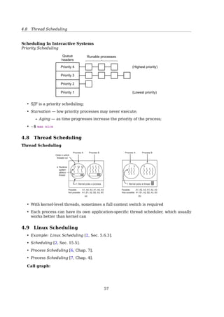
59. 4.8 Thread Scheduling
• SJF is a priority scheduling;
• Starvation — low priority processes may never execute;
– Aging — as time progresses increase the priority of the process;
$ man nice
4.8 Thread Scheduling
Thread Scheduling
Process A Process B Process BProcess A
1. Kernel picks a process 1. Kernel picks a thread
Possible: A1, A2, A3, A1, A2, A3
Also possible: A1, B1, A2, B2, A3, B3
Possible: A1, A2, A3, A1, A2, A3
Not possible: A1, B1, A2, B2, A3, B3
(a) (b)
Order in which
threads run
2. Runtime
system
picks a
thread
1 2 3 1 3 2
Fig. 2-43. (a) Possible scheduling of user-level threads with a 50-
msec process quantum and threads that run 5 msec per CPU burst.
(b) Possible scheduling of kernel-level threads with the same
characteristics as (a).
• With kernel-level threads, sometimes a full context switch is required
• Each process can have its own application-specific thread scheduler, which usually
works better than kernel can
4.9 Linux Scheduling
• [17, Sec. 5.6.3, Example: Linux Scheduling].
• [17, Sec. 15.5, Scheduling].
• [2, Chap. 7, Process Scheduling].
• [11, Chap. 4, Process Scheduling].
Call graph:
cpu_idle()
schedule()
context_switch()
switch_to()
Process Scheduling In Linux
A preemptive, priority-based algorithm with two separate priority ranges:
1. real-time range (0 ∼ 99), for tasks where absolute priorities are more important than
fairness
59

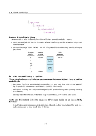
60. 4.9 Linux Scheduling
2. nice value range (100 ∼ 139), for fair preemptive scheduling among multiple processes
In Linux, Process Priority is Dynamic
The scheduler keeps track of what processes are doing and adjusts their priorities
periodically
• Processes that have been denied the use of a CPU for a long time interval are boosted
by dynamically increasing their priority (usually I/O-bound)
• Processes running for a long time are penalized by decreasing their priority (usually
CPU-bound)
• Priority adjustments are performed only on user tasks, not on real-time tasks
Tasks are determined to be I/O-bound or CPU-bound based on an interactivity
heuristic
A task’s interactiveness metric is calculated based on how much time the task exe-
cutes compared to how much time it sleeps
Problems With The Pre-2.6 Scheduler
• an algorithm with O(n) complexity
• a single runqueue for all processors
– good for load balancing
– bad for CPU caches, when a task is rescheduled from one CPU to another
• a single runqueue lock — only one CPU working at a time
The scheduling algorithm used in earlier versions of Linux was quite simple and straight-
forward: at every process switch the kernel scanned the list of runnable processes, com-
puted their priorities, and selected the ”best” process to run. The main drawback of that
algorithm is that the time spent in choosing the best process depends on the number of
runnable processes; therefore, the algorithm is too costly, that is, it spends too much time
in high-end systems running thousands of processes[2, Sec. 7.2, The Scheduling Algo-
rithm].
60

61. 4.9 Linux Scheduling
Scheduling In Linux 2.6 Kernel
• O(1) — Time for finding a task to execute depends not on the number of active tasks
but instead on the number of priorities
• Each CPU has its own runqueue, and schedules itself independently; better cache
efficiency
• The job of the scheduler is simple — Choose the task on the highest priority list to
execute
How to know there are processes waiting in a priority list?
A priority bitmap (5 32-bit words for 140 priorities) is used to define when tasks are on a
given priority list.
• find-first-bit-set instruction is used to find the highest priority bit.
Scheduling In Linux 2.6 Kernel
Each runqueue has two priority arrays
4.9.1 Completely Fair Scheduling
Completely Fair Scheduling (CFS)
Linux’s Process Scheduler
up to 2.4: simple, scaled poorly
• O(n)
• non-preemptive
• single run queue (cache? SMP?)
from 2.5 on: O(1) scheduler
140 priority lists — scaled well
one run queue per CPU — true SMP support
preemptive
ideal for large server workloads
showed latency on desktop systems
from 2.6.23 on: Completely Fair Scheduler (CFS)
improved interactive performance
61

62. 4.9 Linux Scheduling
up to 2.4: The scheduling algorithm used in earlier versions of Linux was quite simple
and straightforward: at every process switch the kernel scanned the list of runnable
processes, computed their priorities, and selected the ”best” process to run. The
main drawback of that algorithm is that the time spent in choosing the best pro-
cess depends on the number of runnable processes; therefore, the algorithm is too
costly, that is, it spends too much time in high-end systems running thousands of
processes[2, Sec. 7.2, The Scheduling Algorithm].
No true SMP all processes share the same run-queue
Cold cache if a process is re-scheduled to another CPU
Completely Fair Scheduler (CFS)
For a perfect (unreal) multitasking CPU
• n runnable processes can run at the same time
• each process should receive 1
n of CPU power
For a real world CPU
• can run only a single task at once — unfair
while one task is running
the others have to wait
• p-wait_runtime is the amount of time the task should now run on the CPU for it
becomes completely fair and balanced.
on ideal CPU, the p-wait_runtime value would always be zero
• CFS always tries to run the task with the largest p-wait_runtime value
See also: Discussing the Completely Fair Scheduler6
CFS
In practice it works like this:
• While a task is using the CPU, its wait_runtime decreases
wait_runtime = wait_runtime - time_running
if: its wait_runtime ̸= MAXwait_runtime (among all processes)
then: it gets preempted
• Newly woken tasks (wait_runtime = 0) are put into the tree more and more to the
right
• slowly but surely giving a chance for every task to become the “leftmost task” and
thus get on the CPU within a deterministic amount of time
References
[1] Wikipedia. Scheduling (computing) — Wikipedia, The Free Encyclopedia. [Online;
accessed 21-February-2015]. 2015.
6http://kerneltrap.org/node/8208
62

63. 5 Deadlock
5.1 Resources
A Major Class of Deadlocks Involve Resources
Processes need access to resources in reasonable order
Suppose...
• a process holds resource A and requests resource B. At same time,
• another process holds B and requests A
Both are blocked and remain so
Examples of computer resources
• printers
• memory space
• data (e.g. a locked record in a DB)
• semaphores
Resources
typedef int semaphore;
semaphore resource 1; semaphore resource 1;
semaphore resource 2; semaphore resource 2;
void process A(void) { void process A(void) {
down(resource 1); down(resource 1);
down(resource 2); down(resource 2);
use both resources( ); use both resources( );
up(resource 2); up(resource 2);
up(resource 1); up(resource 1);
} }
void process B(void) { void process B(void) {
down(resource 1); down(resource 2);
down(resource 2); down(resource 1);
use both resources( ); use both resources( );
up(resource 2); up(resource 1);
up(resource 1); up(resource 2);
} }
(a) (b)
Fig. 3-2. (a) Deadlock-free code. (b) Code with a potential
deadlock.
D
eadlock!
63

64. 5.2 Introduction to Deadlocks
Resources
Deadlocks occur when ...
processes are granted exclusive access to resources
e.g. devices, data records, files, ...
Preemptable resources can be taken away from a process with no ill effects
e.g. memory
Nonpreemptable resources will cause the process to fail if taken away
e.g. CD recorder
In general, deadlocks involve nonpreemptable resources.
Resources
Sequence of events required to use a resource
request « use « release
open() close()
allocate() free()
What if request is denied?
Requesting process
• may be blocked
• may fail with error code
5.2 Introduction to Deadlocks
The Best Illustration of a Deadlock
A law passed by the Kansas legislature early in the 20th century
“When two trains approach each other at a crossing, both shall come to a full stop and
neither shall start up again until the other has gone.”
Introduction to Deadlocks
Deadlock
A set of processes is deadlocked if each process in the set is waiting for an event that only
another process in the set can cause.
• Usually the event is release of a currently held resource
• None of the processes can ...
– run
– release resources
– be awakened
64

65. 5.3 Deadlock Modeling
Four Conditions For Deadlocks
Mutual exclusion condition each resource can only be assigned to one process or is
available
Hold and wait condition process holding resources can request additional
No preemption condition previously granted resources cannot forcibly taken away
Circular wait condition
• must be a circular chain of 2 or more processes
• each is waiting for resource held by next member of the chain
Four Conditions For Deadlocks
Unlocking a deadlock is to answer 4 questions:
1. Can a resource be assigned to more than one process at once?
2. Can a process hold a resource and ask for another?
3. can resources be preempted?
4. Can circular waits exits?
5.3 Deadlock Modeling
Resource-Allocation Graph
(a) (b) (c)
T U
D
C
S
B
A
R
Fig. 3-3. Resource allocation graphs. (a) Holding a resource.
(b) Requesting a resource. (c) Deadlock.
has wants
Strategies for dealing with Deadlocks
1. detection and recovery
2. dynamic avoidance — careful resource allocation
3. prevention — negating one of the four necessary conditions
4. just ignore the problem altogether
65

66. 5.4 Deadlock Detection and Recovery
Resource-Allocation Graph
• The right graph has deadlock
Resource-Allocation Graph
Basic facts:
• No cycles « no deadlock
• If graph contains a cycle «
– if only one instance per resource type, then deadlock
– if several instances per resource type, possibility of
deadlock
5.4 Deadlock Detection and Recovery
Deadlock Detection
• Allow system to enter deadlock state
• Detection algorithm
• Recovery scheme
Deadlock Detection
Single Instance of Each Resource Type — Wait-for Graph
• Pi → Pj if Pi is waiting for Pj;
66

67. 5.4 Deadlock Detection and Recovery
• Periodically invoke an algorithm that searches for a cycle in the graph. If there is a
cycle, there exists a deadlock.
• An algorithm to detect a cycle in a graph requires an order of n2
operations, where n
is the number of vertices in the graph.
Deadlock Detection
Several Instances of a Resource Type
Tape
drives
PlottersScannersC
D
R
om
s
E = ( 4 2 3 1 )
Tape
drives
PlottersScannersC
D
R
om
s
A = ( 2 1 0 0 )
Current allocation matrix
0
2
0
0
0
1
1
0
2
0
1
0
Request matrix
2
1
2
0
0
1
0
1
0
1
0
0
R =C =
Fig. 3-7. An example for the deadlock detection algorithm.Row n:
C: current allocation to process n
R: current requirement of process n
Column m:
C: current allocation of resource class m
R: current requirement of resource class m
Deadlock Detection
Several Instances of a Resource Type
Resources in existence
(E1, E2, E3, …, Em)
Current allocation matrix
C11
C21
Cn1
C12
C22
Cn2
C13
C23
Cn3
C1m
C2m
Cnm
Row n is current allocation
to process n
Resources available
(A1, A2, A3, …, Am)
Request matrix
R11
R21
Rn1
R12
R22
Rn2
R13
R23
Rn3
R1m
R2m
Rnm
Row 2 is what process 2 needs
Fig. 3-6. The four data structures needed by the deadlock detection
algorithm.
n∑
i=1
Cij + Aj = Ej
e.g.
(C13 + C23 + . . . + Cn3) + A3 = E3
n: number of processes;
m: number of resource classes;
67

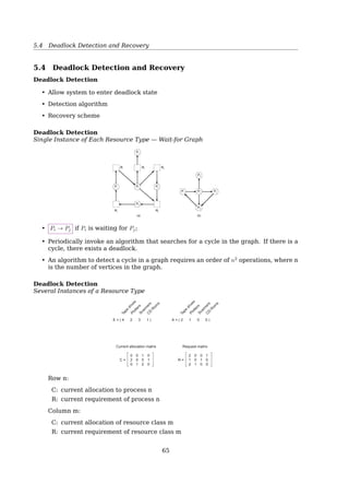
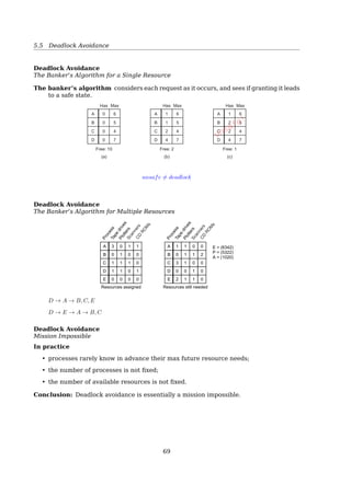
68. 5.4 Deadlock Detection and Recovery
E: a vector of existing resources
• E = [E1, E2, ..., Em]
• Ei = 2 means system has 2 resources of class i, (1 ≤ i ≤ m);
A: a vector of available resources;
• A = [A1, A2, ...Am]
• Ai = 2 means system has 2 resources of class i left unassigned;
Cij: is the number of instances of resource j that process i holds;
e.g. C31 = 2 means P3 has 2 resources of class 1;
Rij: is the number of instances of resource j that process i wants;
e.g. R43 = 2 means P4 wants 2 resources of class 3;
Maths recall: vectors comparison
For two vectors, X and Y
X ≤ Y iff Xi ≤ Yi for 0 ≤ i ≤ m
e.g. [
1 2 3 4
]
≤
[
2 3 4 4
]
[
1 2 3 4
]
≰
[
2 3 2 4
]
Deadlock Detection
Several Instances of a Resource Type
Tape
drives
PlottersScannersC
D
R
om
s
E = ( 4 2 3 1 )
Tape
drives
PlottersScannersC
D
R
om
s
A = ( 2 1 0 0 )
Current allocation matrix
0
2
0
0
0
1
1
0
2
0
1
0
Request matrix
2
1
2
0
0
1
0
1
0
1
0
0
R =C =
Fig. 3-7. An example for the deadlock detection algorithm.
A R
(2 1 0 0) ≥ R3, (2 1 0 0)
(2 2 2 0) ≥ R2, (1 0 1 0)
(4 2 2 1) ≥ R1, (2 0 0 1)
68

69. 5.5 Deadlock Avoidance
Recovery From Deadlock
• Recovery through preemption
– take a resource from some other process
– depends on nature of the resource
• Recovery through rollback
– checkpoint a process periodically
– use this saved state
– restart the process if it is found deadlocked
• Recovery through killing processes
5.5 Deadlock Avoidance
Deadlock Avoidance
Resource Trajectories
Plotter
Printer
Printer
Plotter
B
A
u (Both processes
finished)
p q
r
s
t
I8
I7
I6
I5
I4I3I2I1
;;
;;
;;;
dead
zone
Unsafe region
• B is requesting a resource at point t. The system must decide whether to grant it or
not.
• Deadlock is unavoidable if you get into unsafe region.
Deadlock Avoidance
Safe and Unsafe States
Assuming E = 10
Unsafe
A
B
C
3
2
2
9
4
7
Free: 3
(a)
A
B
C
4
2
2
9
4
7
Free: 2
(b)
A
B
C
4
4 —4
2
9
7
Free: 0
(c)
A
B
C
4
—
2
9
7
Free: 4
(d)
Has Max Has Max Has Max Has Max
Fig. 3-10. Demonstration that the state in (b) is not safe.
unsafe
Safe
69

70. 5.5 Deadlock Avoidance
A
B
C
3
2
2
9
4
7
Free: 3
(a)
A
B
C
3
4
2
9
4
7
Free: 1
(b)
A
B
C
3
0 ––
2
9
7
Free: 5
(c)
A
B
C
3
0
7
9
7
Free: 0
(d)
–
A
B
C
3
0
0
9
–
Free: 7
(e)
Has Max Has Max Has Max Has Max Has Max
Fig. 3-9. Demonstration that the state in (a) is safe.
1. Given totally 10 resources, for process A, B, C:
• A has 3, and need 6 more
• B has 2, and need 2 more
• C has 2, and need 5 more
• 3 left available
2. allocate 1 to A,
• A has 4, and need 5 more
• B unchange
• C unchange
• 2 left available
3. ...
Deadlock Avoidance
The Banker’s Algorithm for a Single Resource
The banker’s algorithm considers each request as it occurs, and sees if granting it leads
to a safe state.
A
B
C
D
0
0
0
0
6
Has Max
5
4
7
Free: 10
A
B
C
D
1
1
2
4
6
Has Max
5
4
7
Free: 2
A
B
C
D
1
2
2
4
6
Has Max
5
4
7
Free: 1
(a) (b) (c)
Fig. 3-11. Three resource allocation states: (a) Safe. (b) Safe.
(c) Unsafe.
unsafe!
unsafe ̸= deadlock
Deadlock Avoidance
The Banker’s Algorithm for Multiple Resources
ProcessTape
drives
Plotters
A
B
C
D
E
3
0
1
1
0
0
1
1
1
0
1
0
1
0
0
1
0
0
1
0
E = (6342)
P = (5322)
A = (1020)
Resources assigned
ProcessTape
drives
Plotters
A
B
C
D
E
1
0
3
0
2
1
1
1
0
1
0
1
0
1
1
0
2
0
0
0
Resources still needed
ScannersCD
RO
M
s
ScannersCD
RO
M
s
Fig. 3-12. The banker’s algorithm with multiple resources.70

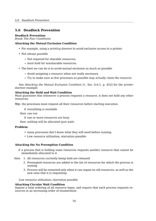
71. 5.6 Deadlock Prevention
D → A → B, C, E
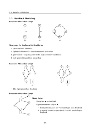
D → E → A → B, C
Deadlock Avoidance
Mission Impossible
In practice
• processes rarely know in advance their max future resource needs;
• the number of processes is not fixed;
• the number of available resources is not fixed.
Conclusion: Deadlock avoidance is essentially a mission impossible.
5.6 Deadlock Prevention
Deadlock Prevention
Break The Four Conditions
Attacking the Mutual Exclusion Condition
• For example, using a printing daemon to avoid exclusive access to a printer.
• Not always possible
– Not required for sharable resources;
– must hold for nonsharable resources.
• The best we can do is to avoid mutual exclusion as much as possible
– Avoid assigning a resource when not really necessary
– Try to make sure as few processes as possible may actually claim the resource
See also: [19, Sec. 6.6.1, Attacking the Mutual Exclusion Condition, p. 452] for the
printer daemon example.
Attacking the Hold and Wait Condition
Must guarantee that whenever a process requests a resource, it does not hold any other
resources.
Try: the processes must request all their resources before starting execution
if everything is available
then can run
if one or more resources are busy
then nothing will be allocated (just wait)
Problem:
• many processes don’t know what they will need before running
• Low resource utilization; starvation possible
71

72. 5.7 The Ostrich Algorithm
Attacking the No Preemption Condition
if a process that is holding some resources requests another resource that cannot be
immediately allocated to it
then 1. All resources currently being held are released
2. Preempted resources are added to the list of resources for which the process is
waiting
3. Process will be restarted only when it can regain its old resources, as well as the
new ones that it is requesting
Low resource utilization; starvation possible
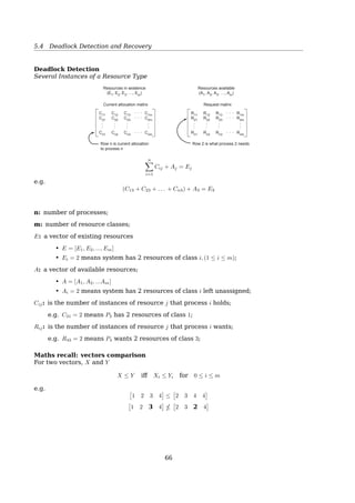
Attacking Circular Wait Condition
Impose a total ordering of all resource types, and require that each process requests re-
sources in an increasing order of enumeration
A1. Imagesetter
2. Scanner
3. Plotter
4. Tape drive
5. CD Rom drive
i
B
j
(a) (b)
Fig. 3-13. (a) Numerically ordered resources. (b) A resource
graph.
It’s hard to find an ordering that satisfies everyone.
5.7 The Ostrich Algorithm
The Ostrich Algorithm
• Pretend there is no problem
• Reasonable if
– deadlocks occur very rarely
– cost of prevention is high
• UNIX and Windows takes this approach
• It is a trade off between
– convenience
– correctness
References
[1] Wikipedia. Deadlock — Wikipedia, The Free Encyclopedia. [Online; accessed 21-
February-2015]. 2015.
6 Memory Management
72

73. 6.1 Background
6.1 Background
Memory Management
In a perfect world Memory is large, fast, non-volatile
In real world ...
Registers
Cache
Main memory
Magnetic tape
Magnetic disk
1 nsec
2 nsec
10 nsec
10 msec
100 sec
1 KB
1 MB
64-512 MB
5-50 GB
20-100 GB
Typical capacityTypical access time
Fig. 1-7. A typical memory hierarchy. The numbers are very rough
approximations.
Memory manager handles the memory hierarchy.
Basic Memory Management
Real Mode
In the old days ...
• Every program simply saw the physical memory
• mono-programming without swapping or paging
(a) (b) (c)
0xFFF …
0 0 0
User
program
User
program
User
program
Operating
system in
RAM
Operating
system in
RAM
Operating
system in
ROM
Device
drivers in ROM
Fig. 4-1. Three simple ways of organizing memory with an operat-
ing system and one user process. Other possibilities also exist.
old mainstream handhold, embedded MS-DOS
Basic Memory Management
Relocation Problem
73

74. 6.1 Background
Exposing
physical memory
to
processes
is not
a good idea
(a) only one program in memory
(b) only another program in memory
(c) both in memory
Memory Protection
Protected mode
We need
• Protect the OS from access by user programs
• Protect user programs from one another
Protected mode is an operational mode of x86-compatible CPU.
• The purpose is to protect everyone else (including the OS) from your program.
Memory Protection
Logical Address Space
Base register holds the smallest legal physical memory address
Limit register contains the size of the range
74

75. 6.1 Background
Registers that are built into the CPU are generally accessible within one
e of the CPU clock. Most CPUs can decode instructions and perform simple
ations on register contents at the rate of one or more operations per
k tick. The same cannot be said of main memory, which is accessed via
ansaction on the memory bus. Completing a memory access may take
y cycles of the CPU clock. In such cases, the processor normally needs
all, since it does not have the data required to complete the instruction
it is executing. This situation is intolerable because of the frequency of
mory accesses. The remedy is to add fast memory between the CPU and
operating
system
0
256000
300040 300040
base
120900
limit
420940
880000
1024000
process
process
process
Figure 7.1 A base and a limit register define a logical address space.
A pair of base and limit registers define
the logical address space
JMP 28
«
JMP 300068
Memory Protection
Base and limit registers
system from access by user processes and, in addition, to protect user processes
from one another. This protection must be provided by the hardware. It can be
implemented in several ways, as we shall see throughout the chapter. In this
section, we outline one possible implementation.
We first need to make sure that each process has a separate memory space.
To do this, we need the ability to determine the range of legal addresses that
the process may access and to ensure that the process can access only these
legal addresses. We can provide this protection by using two registers, usually
a base and a limit, as illustrated in Figure 7.1. The base register holds the
smallest legal physical memory address; the limit register specifies the size of
the range. For example, if the base register holds 300040 and the limit register is
120900, then the program can legally access all addresses from 300040 through
420939 (inclusive).
Protection of memory space is accomplished by having the CPU hardware
compare every address generated in user mode with the registers. Any attempt
by a program executing in user mode to access operating-system memory or
other users’ memory results in a trap to the operating system, which treats the
attempt as a fatal error (Figure 7.2). This scheme prevents a user program from
(accidentally or deliberately) modifying the code or data structures of either
the operating system or other users.
The base and limit registers can be loaded only by the operating system,
which uses a special privileged instruction. Since privileged instructions can
be executed only in kernel mode, and since only the operating system executes
in kernel mode, only the operating system can load the base and limit registers.
This scheme allows the operating system to change the value of the registers
but prevents user programs from changing the registers’ contents.
The operating system, executing in kernel mode, is given unrestricted
access to both operating system memory and users’ memory. This provision
allows the operating system to load users’ programs into users’ memory, to
base
memory
trap to operating system
monitor—addressing error
address yesyes
nono
CPU
base ϩ limit
≥
Figure 7.2 Hardware address protection with base and limit registers.
UNIX View of a Process’ Memory
max +------------------+
| Stack | Stack segment
+--------+---------+
| | |
| v |
| |
| ^ |
| | |
+--------+---------+
| Dynamic storage | Heap
|(from new, malloc)|
+------------------+
| Static variables |
| (uninitialized, | BSS segment
| initialized) | Data segment
+------------------+
| Code | Text segment
0 +------------------+
the size (text + data + bss) of
a process is established at
compile time
text: program code
data: initialized global and static data
bss: uninitialized global and static data
heap: dynamically allocated with malloc, new
stack: local variables
Stack vs. Heap
75

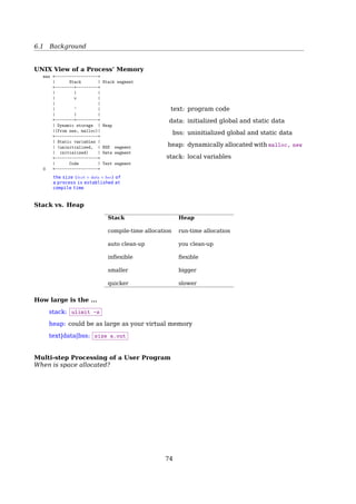
76. 6.1 Background
Stack Heap
compile-time allocation run-time allocation
auto clean-up you clean-up
inflexible flexible
smaller bigger
quicker slower
How large is the ...
stack: ulimit -s
heap: could be as large as your virtual memory
text|data|bss: size a.out
Multi-step Processing of a User Program
When is space allocated?
7.1 Background 281
dynamic
linking
source
program
object
module
linkage
editor
load
module
loader
in-memory
binary
memory
image
other
object
modules
compile
time
load
time
execution
time (run
time)
compiler or
assembler
system
library
dynamically
loaded
system
library
Figure 7.3 Multistep processing of a user program.
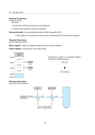
7.1.3 Logical Versus Physical Address Space
An address generated by the CPU is commonly referred to as a logical address,
whereas an address seen by the memory unit—that is, the one loaded into
the memory-address register of the memory—is commonly referred to as a
physical address.
The compile-time and load-time address-binding methods generate iden-
tical logical and physical addresses. However, the execution-time address-
binding scheme results in differing logical and physical addresses. In this case,
we usually refer to the logical address as a virtual address. We use logical address
and virtual address interchangeably in this text. The set of all logical addresses
generated by a program is a logical address space; the set of all physical
addresses corresponding to these logical addresses is a physical address space.
Thus, in the execution-time address-binding scheme, the logical and physical
address spaces differ.
The run-time mapping from virtual to physical addresses is done by a
hardware device called the memory-management unit (MMU). We can choose
from many different methods to accomplish thsi mapping, as we discuss in
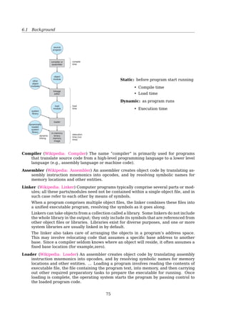
Static: before program start running
• Compile time
• Load time
Dynamic: as program runs
• Execution time
Compiler The name ”compiler” is primarily used for programs that translate source code
from a high-level programming language to a lower level language (e.g., assembly
language or machine code)[22].
Assembler An assembler creates object code by translating assembly instruction mnemon-
ics into opcodes, and by resolving symbolic names for memory locations and other
entities[21].
76

77. 6.1 Background
Linker Computer programs typically comprise several parts or modules; all these parts/modules
need not be contained within a single object file, and in such case refer to each other
by means of symbols[30].
When a program comprises multiple object files, the linker combines these files into
a unified executable program, resolving the symbols as it goes along.
Linkers can take objects from a collection called a library. Some linkers do not include
the whole library in the output; they only include its symbols that are referenced from
other object files or libraries. Libraries exist for diverse purposes, and one or more
system libraries are usually linked in by default.
The linker also takes care of arranging the objects in a program’s address space.
This may involve relocating code that assumes a specific base address to another
base. Since a compiler seldom knows where an object will reside, it often assumes a
fixed base location (for example,zero).
Loader An assembler creates object code by translating assembly instruction mnemon-
ics into opcodes, and by resolving symbolic names for memory locations and other
entities. ... Loading a program involves reading the contents of executable file, the
file containing the program text, into memory, and then carrying out other required
preparatory tasks to prepare the executable for running. Once loading is complete,
the operating system starts the program by passing control to the loaded program
code[31].
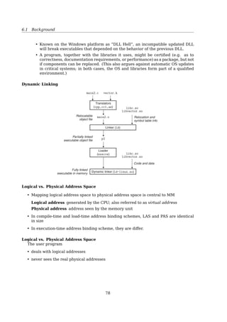
Dynamic linker A dynamic linker is the part of an operating system (OS) that loads
(copies from persistent storage to RAM) and links (fills jump tables and relocates
pointers) the shared libraries needed by an executable at run time, that is, when it is
executed. The specific operating system and executable format determine how the
dynamic linker functions and how it is implemented. Linking is often referred to as
a process that is performed at compile time of the executable while a dynamic linker
is in actuality a special loader that loads external shared libraries into a running pro-
cess and then binds those shared libraries dynamically to the running process. The
specifics of how a dynamic linker functions is operating-system dependent[25].
Linkers and Loaders allow programs to be built from modules rather than as one big
monolith.
See also:
• [3, Chap. 7, Linking].
• COMPILER, ASSEMBLER, LINKER AND LOADER: A BRIEF STORY7
• Linkers and Loaders8
• [10, Links and loaders]
• Linux Journal: Linkers and Loaders9
. Discussing how compilers, links and loaders
work and the benefits of shared libraries.
Address Binding
Who assigns memory to segments?
Static-binding: before a program starts running
7http://www.tenouk.com/ModuleW.html
8http://www.iecc.com/linker/
9http://www.linuxjournal.com/article/6463
77

78. 6.1 Background
Compile time: Compiler and assembler generate an object file for each source file
Load time:
• Linker combines all the object files into a single executable object file
• Loader (part of OS) loads an executable object file into memory at location(s)
determined by the OS
- invoked via the execve system call
Dynamic-binding: as program runs
• Execution time:
– uses new and malloc to dynamically allocate memory
– gets space on stack during function calls
• Address binding has nothing to do with physical memory (RAM). It determines the
addresses of objects in the address space (virtual memory) of a process.
Static loading
• The entire program and all data of a process must be in physical memory for the
process to execute
• The size of a process is thus limited to the size of physical memory670 Chapter 7 Linking
main2.c vector.h
libvector.a libc.a
addvec.o printf.o and any other
modules called by printf.o
main2.o
Translators
(cpp, cc1, as)
Linker (ld)
p2 Fully linked
executable object file
Relocatable
object files
Source files
Static libraries
Figure 7.7 Linking with static libraries.
To build the executable, we would compile and link the input files main.o and
libvector.a:
unix gcc -O2 -c main2.c
unix gcc -static -o p2 main2.o ./libvector.a
Figure 7.7 summarizes the activity of the linker. The -static argument tells
the compiler driver that the linker should build a fully linked executable object file
that can be loaded into memory and run without any further linking at load time.
When the linker runs, it determines that the addvec symbol defined by addvec.o
is referenced by main.o, so it copies addvec.o into the executable. Since the
program doesn’t reference any symbols defined by multvec.o, the linker does
not copy this module into the executable. The linker also copies the printf.o
module from libc.a, along with a number of other modules from the C run-time
system.
7.6.3 How Linkers Use Static Libraries to Resolve References
While static libraries are useful and essential tools, they are also a source of
confusion to programmers because of the way the Unix linker uses them to resolve
external references. During the symbol resolution phase, the linker scans the
relocatable object files and archives left to right in the same sequential order that
Dynamic Linking
A dynamic linker is actually a special loader that loads external shared libraries into a
running process
• Small piece of code, stub, used to locate the appropriate memory-resident library
routine
• Only one copy in memory
• Don’t have to re-link after a library update
78

79. 6.1 Background
if ( stub_is_executed ){
if ( !routine_in_memory )
load_routine_into_memory();
stub_replaces_itself_with_routine();
execute_routine();
}
Dynamic linking Many operating system environments allow dynamic linking, that is
the postponing of the resolving of some undefined symbols until a program is run.
That means that the executable code still contains undefined symbols, plus a list of
objects or libraries that will provide definitions for these. Loading the program will
load these objects/libraries as well, and perform a final linking. Dynamic linking
needs no linker[30, Dynamic linking].
This approach offers two advantages:
• Often-used libraries (for example the standard system libraries) need to be stored
in only one location, not duplicated in every single binary.
• If an error in a library function is corrected by replacing the library, all programs
using it dynamically will benefit from the correction after restarting them. Pro-
grams that included this function by static linking would have to be re-linked
first.
There are also disadvantages:
• Known on the Windows platform as ”DLL Hell”, an incompatible updated DLL
will break executables that depended on the behavior of the previous DLL.
• A program, together with the libraries it uses, might be certified (e.g. as to
correctness, documentation requirements, or performance) as a package, but not
if components can be replaced. (This also argues against automatic OS updates
in critical systems; in both cases, the OS and libraries form part of a qualified
environment.)
Dynamic Linking
79

80. 6.1 Background
Section 7.11 Loading and Linking Shared Libraries from Applications 683
Figure 7.15
Dynamic linking with
shared libraries.
main2.c
libc.so
libvector.so
libc.so
libvector.so
main2.o
p2
Translators
(cpp,cc1,as)
Linker (ld)
Fully linked
executable in memory
Partially linked
executable object file
vector.h
Loader
(execve)
Dynamic linker (ld-linux.so)
Relocatable
object file
Relocation and
symbol table info
Code and data
contains a .interp section, which contains the path name of the dynamic linker,
which is itself a shared object (e.g., ld-linux.so on Linux systems). Instead of
passing control to the application, as it would normally do, the loader loads and
runs the dynamic linker.
The dynamic linker then finishes the linking task by performing the following
relocations:
.
Relocating the text and data of libc.so into some memory segment.
.
Relocating the text and data of libvector.so into another memory segment.
.
Relocating any references in p2 to symbols defined by libc.so and libvec-
tor.so.
Finally, the dynamic linker passes control to the application. From this point on,
the locations of the shared libraries are fixed and do not change during execution
of the program.
7.11 Loading and Linking Shared Libraries from Applications
Up to this point, we have discussed the scenario in which the dynamic linker loads
and links shared libraries when an application is loaded, just before it executes.
However, it is also possible for an application to request the dynamic linker to
load and link arbitrary shared libraries while the application is running, without
having to link in the applications against those libraries at compile time.
Logical vs. Physical Address Space
• Mapping logical address space to physical address space is central to MM
Logical address generated by the CPU; also referred to as virtual address
Physical address address seen by the memory unit
• In compile-time and load-time address binding schemes, LAS and PAS are identical
in size
• In execution-time address binding scheme, they are differ.
Logical vs. Physical Address Space
The user program
• deals with logical addresses
• never sees the real physical addresses282 Chapter 7 Main Memory
ϩ
MMU
CPU memory
14346
14000
relocation
register
346
logical
address
physical
address
Figure 7.4 Dynamic relocation using a relocation register.
Sections 7.3 through 7.7. For the time being, we illustrate this mapping with
a simple MMU scheme that is a generalization of the base-register scheme
described in Section 7.1.1. The base register is now called a relocation register.
The value in the relocation register is added to every address generated by a user
process at the time the address is sent to memory (see Figure 7.4). For example,
if the base is at 14000, then an attempt by the user to address location 0 is
dynamically relocated to location 14000; an access to location 346 is mapped
80

81. 6.1 Background
MMU
Memory Management Unit
CPU
package
CPU
The CPU sends virtual
addresses to the MMU
The MMU sends physical
addresses to the memory
Memory
management
unit
Memory
Disk
controller
Bus
Fig. 4-9. The position and function of the MMU. Here the MMU
is shown as being a part of the CPU chip because it commonly is
nowadays. However, logically it could be a separate chip and was
in years gone by.
Memory Protection
memory mapping and protection. We can provide these features by using a
relocation register, as discussed in Section 7.1.3, together with a limit register,
as discussed in Section 7.1.1. The relocation register contains the value of
the smallest physical address; the limit register contains the range of logical
addresses (for example, relocation = 100040 and limit = 74600). With relocation
and limit registers, each logical address must be less than the limit register; the
MMU maps the logical address dynamically by adding the value in the relocation
register. This mapped address is sent to memory (Figure 7.6).
When the CPU scheduler selects a process for execution, the dispatcher
loads the relocation and limit registers with the correct values as part of the
context switch. Because every address generated by a CPU is checked against
these registers, we can protect both the operating system and other users’
programs and data from being modified by this running process.
The relocation-register scheme provides an effective way to allow the
operating system’s size to change dynamically. This flexibility is desirable in
many situations. For example, the operating system contains code and buffer
space for device drivers. If a device driver (or other operating-system service)
is not commonly used, we do not want to keep the code and data in memory, as
we might be able to use that space for other purposes. Such code is sometimes
called transient operating-system code; it comes and goes as needed. Thus,
using this code changes the size of the operating system during program
execution.
7.3.2 Memory Allocation
Now we are ready to turn to memory allocation. One of the simplest
methods for allocating memory is to divide memory into several fixed-sized
partitions. Each partition may contain exactly one process. Thus, the degree
CPU memory
logical
address
trap: addressing error
no
yes
physical
address
relocation
register
ϩϽ
limit
register
Figure 7.6 Hardware support for relocation and limit registers.
Swapping
284 Chapter 7 Main Memory
in it. Other programs linked before the new library was installed will continue
using the older library. This system is also known as shared libraries.
Unlike dynamic loading, dynamic linking generally requires help from the
operating system. If the processes in memory are protected from one another,
then the operating system is the only entity that can check to see whether the
needed routine is in another process’s memory space or that can allow multiple
processes to access the same memory addresses. We elaborate on this concept
when we discuss paging in Section 7.4.4.
7.2 Swapping
A process must be in memory to be executed. A process, however, can be
swapped temporarily out of memory to a backing store and then brought
back into memory for continued execution. For example, assume a multipro-
gramming environment with a round-robin CPU-scheduling algorithm. When
a quantum expires, the memory manager will start to swap out the process that
just finished and to swap another process into the memory space that has been
freed (Figure 7.5). In the meantime, the CPU scheduler will allocate a time slice
to some other process in memory. When each process finishes its quantum, it
will be swapped with another process. Ideally, the memory manager can swap
processes fast enough that some processes will be in memory, ready to execute,
when the CPU scheduler wants to reschedule the CPU. In addition, the quantum
must be large enough to allow reasonable amounts of computing to be done
between swaps.
A variant of this swapping policy is used for priority-based scheduling
algorithms. If a higher-priority process arrives and wants service, the memory
manager can swap out the lower-priority process and then load and execute
the higher-priority process. When the higher-priority process finishes, the
operating
system
swap out
swap in
user
space
main memory
backing store
process P2
process P1
1
2
Figure 7.5 Swapping of two processes using a disk as a backing store.
Major part of swap time is transfer time
Total transfer time is directly proportional to the amount of memory swapped
81

82. 6.2 Contiguous Memory Allocation
6.2 Contiguous Memory Allocation
Contiguous Memory Allocation
Multiple-partition allocation
(a)
Operating
system
;;
;;
A
(b)
Operating
system
;;
;;A
B
(c)
Operating
system
;A
B
C
(d)
Time
Operating
system;;
;;;;
;;B
C
(e)
D
Operating
system
;;
;;
B
C
(f)
D
Operating
system
;;
;;;
;;
C
(g)
D
Operating
system
;
A
C
Fig. 4-5. Memory allocation changes as processes come into
memory and leave it. The shaded regions are unused memory.
Operating system maintains information about:
a allocated partitions
b free partitions (hole)
Dynamic Storage-Allocation Problem
First Fit, Best Fit, Worst Fit
1000 10000 5000 200
150
150 1509850
leftover
50
leftover
first
fit
worst fit
best fit
First-fit: The first hole that is big enough
Best-fit: The smallest hole that is big enough
• Must search entire list, unless ordered by size
• Produces the smallest leftover hole
Worst-fit: The largest hole
• Must also search entire list
• Produces the largest leftover hole
• First-fit and best-fit better than worst-fit in terms of speed and storage utilization
• First-fit is generally faster
82

83. 6.3 Virtual Memory
Fragmentation
Process
A
Process
B
Process
C
Internal
Fragmentation
external
Fragmentation
Reduce external fragmentation by
• Compaction is possible only if relocation is dynamic,
and is done at execution time
• Noncontiguous memory allocation
– Paging
– Segmentation
6.3 Virtual Memory
Virtual Memory
Logical memory can be much larger than physical memory
Virtual
address
space
Physical
memory
address
60K-64K
56K-60K
52K-56K
48K-52K
44K-48K
40K-44K
36K-40K
32K-36K
28K-32K
24K-28K
20K-24K
16K-20K
12K-16K
8K-12K
4K-8K
0K-4K
28K-32K
24K-28K
20K-24K
16K-20K
12K-16K
8K-12K
4K-8K
0K-4K
Virtual page
Page frame
X
X
X
X
7
X
5
X
X
X
3
4
0
6
1
2
Fig. 4-10. The relation between virtual addresses and physical
memory addresses is given by the page table.
Address translation
virtual
address
page table
−−−−−−→
physical
address
Page 0
map to
−−−−→ Frame 2
0virtual
map to
−−−−→ 8192physical
20500vir
(20k + 20)vir
map to
−−−−→
12308phy
(12k + 20)phy
Page Fault
83

84. 6.3 Virtual Memory
Virtual
address
space
Physical
memory
address
60K-64K
56K-60K
52K-56K
48K-52K
44K-48K
40K-44K
36K-40K
32K-36K
28K-32K
24K-28K
20K-24K
16K-20K
12K-16K
8K-12K
4K-8K
0K-4K
28K-32K
24K-28K
20K-24K
16K-20K
12K-16K
8K-12K
4K-8K
0K-4K
Virtual page
Page frame
X
X
X
X
7
X
5
X
X
X
3
4
0
6
1
2
Fig. 4-10. The relation between virtual addresses and physical
memory addresses is given by the page table.
MOV REG, 32780 ?
Page fault swapping
6.3.1 Paging
Paging
Address Translation Scheme
Address generated by CPU is divided into:
Page number(p): an index into a page table
Page offset(d): to be copied into memory
Given logical address space (2m
) and page size (2n
),
number of pages =
2m
2n
= 2m−n
Example: addressing to 0010000000000100
m−n=4
0 0 1 0
n=12
0 0 0 0 0 0 0 0 0 1 0 0
m=16
page number = 0010 = 2, page offset = 000000000100
84

85. 6.3 Virtual Memory
15
14
13
12
11
10
9
8
7
6
5
4
3
2
1
0
000
000
000
000
111
000
101
000
000
000
011
100
000
110
001
010
0
0
0
0
1
0
1
0
0
0
1
1
1
1
1
1
Present/
absent bit
Page
table
12-bit offset
copied directly
from input
to output
Virtual page = 2 is used
as an index into the
page table Incoming
virtual
address
(8196)
Outgoing
physical
address
(24580)
110
1 1 0 0 0 0 0 0 0 0 0 0 1 0 0
00 1 0 0 0 0 0 0 0 0 0 0 1 0 0
Fig. 4-11. The internal operation of the MMU with 16 4-KB
pages.
Virtual pages: 16
Page size: 4k
Virtual memory: 64K
Physical frames: 8
Physical memory: 32K
Shared Pages 7.5 Structure of the Page Table 299
7
6
5
ed 24
ed 13
2
data 11
0
3
4
6
1
page table
for P1
process P1
data 1
ed 2
ed 3
ed 1
3
4
6
2
page table
for P3
process P3
data 3
ed 2
ed 3
ed 1
3
4
6
7
page table
for P2
process P2
data 2
ed 2
ed 3
ed 1
8
9
10
11
data 3
2data
ed 3
Figure 7.13 Sharing of code in a paging environment.
of interprocess communication. Some operating systems implement shared
memory using shared pages.
Organizing memory according to pages provides numerous benefits in
addition to allowing several processes to share the same physical pages. We
cover several other benefits in Chapter 8.
7.5 Structure of the Page Table
In this section, we explore some of the most common techniques for structuring
the page table.
7.5.1 Hierarchical Paging
Most modern computer systems support a large logical address space
(232
to 264
). In such an environment, the page table itself becomes excessively
large. For example, consider a system with a 32-bit logical address space. If
the page size in such a system is 4 KB (212
), then a page table may consist of
up to 1 million entries (232
/212
). Assuming that each entry consists of 4 bytes,
each process may need up to 4 MB of physical address space for the page table
alone. Clearly, we would not want to allocate the page table contiguously in
main memory. One simple solution to this problem is to divide the page table
into smaller pieces. We can accomplish this division in several ways.
One way is to use a two-level paging algorithm, in which the page table
itself is also paged (Figure 7.14). For example, consider again the system with
Page Table Entry
Intel i386 Page Table Entry
• Commonly 4 bytes (32 bits) long
• Page size is usually 4k (212
bytes). OS dependent
$ getconf PAGESIZE
• Could have 232−12
= 220
= 1M pages
Could address 1M × 4KB = 4GB memory
85

86. 6.3 Virtual Memory
31 12 11 0
+--------------------------------------+-------+---+-+-+---+-+-+-+
| | | | | | |U|R| |
| PAGE FRAME ADDRESS 31..12 | AVAIL |0 0|D|A|0 0|/|/|P|
| | | | | | |S|W| |
+--------------------------------------+-------+---+-+-+---+-+-+-+
P - PRESENT
R/W - READ/WRITE
U/S - USER/SUPERVISOR
A - ACCESSED
D - DIRTY
AVAIL - AVAILABLE FOR SYSTEMS PROGRAMMER USE
NOTE: 0 INDICATES INTEL RESERVED. DO NOT DEFINE.
Page Table
• Page table is kept in main memory
• Usually one page table for each process
• Page-table base register (PTBR): A pointer to the page table is stored in PCB
• Page-table length register (PRLR): indicates size of the page table
• Slow
– Requires two memory accesses. One for the page table and one for the data/instruction.
• TLB
Translation Lookaside Buffer (TLB)
Fact: 80-20 rule
• Only a small fraction of the PTEs are heavily read; the rest are barely used at all
296 Chapter 7 Main Memory
page table
f
CPU
logical
address
p d
f d
physical
address
physical
memory
p
TLB miss
page
number
frame
number
TLB hit
TLB
Figure 7.11 Paging hardware with TLB.
contain valid virtual addresses but have incorrect or invalid physical addresses
left over from the previous process.
The percentage of times that a particular page number is found in the TLB
is called the hit ratio. An 80-percent hit ratio, for example, means that we
find the desired page number in the TLB 80 percent of the time. If it takes 20
nanoseconds to search the TLB and 100 nanoseconds to access memory, then
a mapped-memory access takes 120 nanoseconds when the page number is
in the TLB. If we fail to find the page number in the TLB (20 nanoseconds),
then we must first access memory for the page table and frame number (100
nanoseconds) and then access the desired byte in memory (100 nanoseconds),
for a total of 220 nanoseconds. To find the effective memory-access time, we
weight the case by its probability:
effective access time = 0.80 × 120 + 0.20 × 220
= 140 nanoseconds.
In this example, we suffer a 40-percent slowdown in memory-access time (from
100 to 140 nanoseconds).
Multilevel Page Tables
86

87. 6.3 Virtual Memory
• a 1M-entry page table eats 4M memory
• while 100 processes running, 400M memory
is gone for page tables
• avoid keeping all the page tables in memory
all the time
A two-level scheme:
page number | page offset
+----------+----------+------------+
| p1 | p2 | d |
+----------+----------+------------+
10 10 12
| |
| ‘- pointing to 1k frames
‘-- pointing to 1k page tables
300 Chapter 7 Main Memory
•
•
•
•
•
•
outer page
table
page of
page table
page table
memory
929
900
929
900
708
500
100
1
0
•
•
•
100
708
•
•
•
•
•
•
•
•
•
•
•
•
•
•
•
•
•
•
•
•
•
•
•
•
•
•
•
1
500
Figure 7.14 A two-level page-table scheme.
a 32-bit logical address space and a page size of 4 KB. A logical address is
divided into a page number consisting of 20 bits and a page offset consisting
of 12 bits. Because we page the page table, the page number is further divided
into a 10-bit page number and a 10-bit page offset. Thus, a logical address is as
follows:
p1 p2 d
page number page offset
10 10 12
where p1 is an index into the outer page table and p2 is the displacement
within the page of the inner page table. The address-translation method for this
architecture is shown in Figure 7.15. Because address translation works from
the outer page table inward, this scheme is also known as a forward-mapped
page table.
The VAX architecture supports a variation of two-level paging. The VAX is
a 32-bit machine with a page size of 512 bytes. The logical address space of a
process is divided into four equal sections, each of which consists of 230
bytes.
Each section represents a different part of the logical address space of a process.
The first 2 high-order bits of the logical address designate the appropriate
section. The next 21 bits represent the logical page number of that section, and
the final 9 bits represent an offset in the desired page. By partitioning the page
p1: is an index into the outer page table
p2: is the displacement within the page of the outer page table
• Split one huge page table into 1k small page tables
– i.e. the huge page table has 1k entries.
– Each entry keeps a page frame number of a small page table.
• Each small page table has 1k entries
– Each entry keeps a page frame number of a physical frame.
Two-Level Page Tables
Example
87

88. 6.3 Virtual Memory
Don’t have to keep all the 1K page tables
(1M pages) in memory. In this example
only 4 page tables are actually
mapped into memory
process
+-------+
| stack | 4M
+-------+
| |
| ... | unused
| |
+-------+
| data | 4M
+-------+
| code | 4M
+-------+
Top−level
page table
Second−level
page tables
To
pages
Page
table for
the top
4M of
memory
6
5
4
3
2
1
0
1023
1023
6
5
4
3
2
1
0
1023
Bits 10 10 12
PT1 PT2 Offset
4M−1
8M−1
Page table
Page table
Page table
Page table
Page table
Page table
00000000010000000011000000000100
PT1 = 1 PT2 = 3 Offset = 4
0
1
2
3 929
788
850
Page table
Page table
901
500
Problem With 64-bit Systems
if
• virtual address space = 64 bits
• page size = 4 KB = 212
B
then How much space would a simple single-level page table take?
if Each page table entry takes 4 Bytes
then The whole page table (264−12
entries) will take
264−12
× 4 B = 254
B = 16 PB (peta ⇒ tera ⇒ giga)!
And this is for ONE process!
Multi-level?
if 10 bits for each level
then 64−12
10 = 5 levels are required
5 memory accress for each address translation!
Inverted Page Tables
Index with frame number
Inverted Page Table:
88

89. 6.3 Virtual Memory
• One entry for each physical frame
– The physical frame number is the table index
• A single global page table for all processes
– The table is shared — PID is required
• Physical pages are now mapped to virtual — each entry contains a virtual page num-
ber instead of a physical one
• Information bits, e.g. protection bit, are as usual
Find index according to entry contents
(pid, p) ⇒ i
address, regardless of the latter’s validity). This table representation is a natural
one, since processes reference pages through the pages’ virtual addresses. The
operating system must then translate this reference into a physical memory
address. Since the table is sorted by virtual address, the operating system is
able to calculate where in the table the associated physical address entry is
located and to use that value directly. One of the drawbacks of this method
is that each page table may consist of millions of entries. These tables may
consume large amounts of physical memory just to keep track of how other
physical memory is being used.
To solve this problem, we can use an inverted page table. An inverted
page table has one entry for each real page (or frame) of memory. Each entry
consists of the virtual address of the page stored in that real memory location,
with information about the process that owns the page. Thus, only one page
table is in the system, and it has only one entry for each page of physical
memory. Figure 7.17 shows the operation of an inverted page table. Compare
it with Figure 7.7, which depicts a standard page table in operation. Inverted
page tables often require that an address-space identifier (Section 7.4.2) be
stored in each entry of the page table, since the table usually contains several
different address spaces mapping physical memory. Storing the address-space
identifier ensures that a logical page for a particular process is mapped to the
corresponding physical page frame. Examples of systems using inverted page
tables include the 64-bit UltraSPARC and PowerPC.
To illustrate this method, we describe a simplified version of the inverted
page table used in the IBM RT. Each virtual address in the system consists of a
triple:
process-id, page-number, offset.
Each inverted page-table entry is a pair process-id, page-number where the
process-id assumes the role of the address-space identifier. When a memory
page table
CPU
logical
address physical
address
physical
memory
i
pid p
pid
search
p
d i d
Figure 7.17 Inverted page table.
Std. PTE (32-bit sys.):
page frame address | info
+--------------------+------+
| 20 | 12 |
+--------------------+------+
indexed by page number
if 220
entries, 4 B each
then SIZEpage table = 220
× 4 = 4 MB
(for each process)
Inverted PTE (64-bit sys.):
pid | virtual page number | info
+-----+---------------------+------+
| 16 | 52 | 12 |
+-----+---------------------+------+
indexed by frame number
if assuming
– 16 bits for PID
– 52 bits for virtual page number
– 12 bits of information
then each entry takes 16 + 52 + 12 = 80 bits = 10 bytes
if physical mem = 1G (230
B), and page size =
4K (212
B), we’ll have 230−12
= 218
pages
then SIZEpage table = 218
× 10 B = 2.5 MB
(for all processes)
Inefficient: Require searching the entire table
89

90. 6.3 Virtual Memory
Hashed Inverted Page Tables
A hash anchor table — an extra level before the actual page table
• maps process IDs
virtual page numbers
⇒ page table entries
• Since collisions may occur, the page table must do chaining
302 Chapter 7 Main Memory
The next step would be a four-level paging scheme, where the second-level
outer page table itself is also paged, and so forth. The 64-bit UltraSPARC would
require seven levels of paging—a prohibitive number of memory accesses—
to translate each logical address. You can see from this example why, for 64-bit
architectures, hierarchical page tables are generally considered inappropriate.
7.5.2 Hashed Page Tables
A common approach for handling address spaces larger than 32 bits is to use
a hashed page table, with the hash value being the virtual page number. Each
entry in the hash table contains a linked list of elements that hash to the same
location (to handle collisions). Each element consists of three fields: (1) the
virtual page number, (2) the value of the mapped page frame, and (3) a pointer
to the next element in the linked list.
The algorithm works as follows: The virtual page number in the virtual
address is hashed into the hash table. The virtual page number is compared
with field 1 in the first element in the linked list. If there is a match, the
corresponding page frame (field 2) is used to form the desired physical address.
If there is no match, subsequent entries in the linked list are searched for a
matching virtual page number. This scheme is shown in Figure 7.16.
A variation of this scheme that is favorable for 64-bit address spaces has
been proposed. This variation uses clustered page tables, which are similar to
hashed page tables except that each entry in the hash table refers to several
pages (such as 16) rather than a single page. Therefore, a single page-table
entry can store the mappings for multiple physical-page frames. Clustered
page tables are particularly useful for sparse address spaces, where memory
references are noncontiguous and scattered throughout the address space.
7.5.3 Inverted Page Tables
Usually, each process has an associated page table. The page table has one
entry for each page that the process is using (or one slot for each virtual
hash table
q s
logical address
physical
address
physical
memory
p d r d
p r
hash
function
• • •
Figure 7.16 Hashed page table.
Hashed Inverted Page Table
90

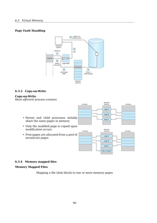
91. 6.3 Virtual Memory
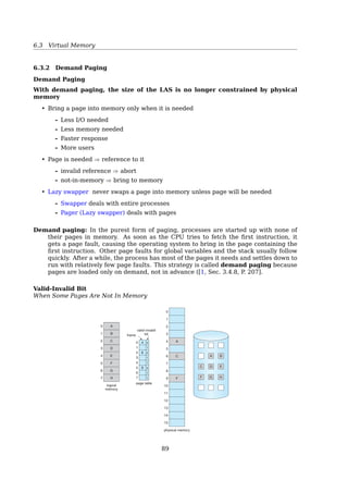
6.3.2 Demand Paging
Demand Paging
With demand paging, the size of the LAS is no longer constrained by physical
memory
• Bring a page into memory only when it is needed
– Less I/O needed
– Less memory needed
– Faster response
– More users
• Page is needed ⇒ reference to it
– invalid reference ⇒ abort
– not-in-memory ⇒ bring to memory
• Lazy swapper never swaps a page into memory unless page will be needed
– Swapper deals with entire processes
– Pager (Lazy swapper) deals with pages
Demand paging: In the purest form of paging, processes are started up with none of
their pages in memory. As soon as the CPU tries to fetch the first instruction, it
gets a page fault, causing the operating system to bring in the page containing the
first instruction. Other page faults for global variables and the stack usually follow
quickly. After a while, the process has most of the pages it needs and settles down to
run with relatively few page faults. This strategy is called demand paging because
pages are loaded only on demand, not in advance ([19, Sec. 3.4.8, P. 207].
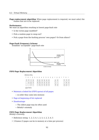
Valid-Invalid Bit
When Some Pages Are Not In Memory
324 Chapter 8 Virtual Memory
8.2.1 Basic Concepts
When a process is to be swapped in, the pager guesses which pages will be
used before the process is swapped out again. Instead of swapping in a whole
process, the pager brings only those pages into memory. Thus, it avoids reading
into memory pages that will not be used anyway, decreasing the swap time
and the amount of physical memory needed.
With this scheme, we need some form of hardware support to distinguish
between the pages that are in memory and the pages that are on the disk.
The valid–invalid bit scheme described in Section 7.4.3 can be used for this
purpose. This time, however, when this bit is set to “valid,” the associated page
is both legal and in memory. If the bit is set to “invalid,” the page either is not
valid (that is, not in the logical address space of the process) or is valid but
is currently on the disk. The page-table entry for a page that is brought into
memory is set as usual, but the page-table entry for a page that is not currently
in memory is either simply marked invalid or contains the address of the page
on disk. This situation is depicted in Figure 8.5.
Notice that marking a page invalid will have no effect if the process never
attempts to access that page. Hence, if we guess right and page in all and only
those pages that are actually needed, the process will run exactly as though we
had brought in all pages. While the process executes and accesses pages that
are memory resident, execution proceeds normally.
B
D
D E
F
H
logical
memory
valid–invalid
bitframe
page table
1
0 4
62
3
4
5 9
6
7
1
0
2
3
4
5
6
7
i
v
v
i
i
v
i
i
physical memory
A
A BC
C
F G HF
1
0
2
3
4
5
6
7
9
8
10
11
12
13
14
15
A
C
E
G
Figure 8.5 Page table when some pages are not in main memory.
91

92. 6.3 Virtual Memory
Page Fault Handling 8.2 Demand Paging 325
load M
reference
trap
i
page is on
backing store
operating
system
restart
instruction
reset page
table
page table
physical
memory
bring in
missing page
free frame
1
2
3
6
5 4
Figure 8.6 Steps in handling a page fault.
But what happens if the process tries to access a page that was not brought
into memory? Access to a page marked invalid causes a page fault. The paging
hardware, in translating the address through the page table, will notice that
the invalid bit is set, causing a trap to the operating system. This trap is the
result of the operating system’s failure to bring the desired page into memory.
The procedure for handling this page fault is straightforward (Figure 8.6):
1. We check an internal table (usually kept with the process control block)
for this process to determine whether the reference was a valid or an
invalid memory access.
2. If the reference was invalid, we terminate the process. If it was valid, but
we have not yet brought in that page, we now page it in.
3. We find a free frame (by taking one from the free-frame list, for example).
4. We schedule a disk operation to read the desired page into the newly
allocated frame.
5. When the disk read is complete, we modify the internal table kept with
the process and the page table to indicate that the page is now in memory.
6. We restart the instruction that was interrupted by the trap. The process
can now access the page as though it had always been in memory.
In the extreme case, we can start executing a process with no pages in
memory. When the operating system sets the instruction pointer to the first
6.3.3 Copy-on-Write
Copy-on-Write
More efficient process creation
• Parent and child processes initially
share the same pages in memory
• Only the modified page is copied upon
modification occurs
• Free pages are allocated from a pool of
zeroed-out pages
330 Chapter 8 Virtual Memory
process1
physical
memory
page A
page B
page C
process2
Figure 8.7 Before process 1 modifies page C.
Recall that the fork() system call creates a child process that is a duplicate
of its parent. Traditionally, fork() worked by creating a copy of the parent’s
address space for the child, duplicating the pages belonging to the parent.
However, considering that many child processes invoke the exec() system
call immediately after creation, the copying of the parent’s address space may
be unnecessary. Instead, we can use a technique known as copy-on-write,
which works by allowing the parent and child processes initially to share the
same pages. These shared pages are marked as copy-on-write pages, meaning
that if either process writes to a shared page, a copy of the shared page is
created. Copy-on-write is illustrated in Figures 8.7 and Figure 8.8, which show
the contents of the physical memory before and after process 1 modifies page
C.
For example, assume that the child process attempts to modify a page
containing portions of the stack, with the pages set to be copy-on-write. The
operating system will create a copy of this page, mapping it to the address space
of the child process. The child process will then modify its copied page and not
the page belonging to the parent process. Obviously, when the copy-on-write
technique is used, only the pages that are modified by either process are copied;
all unmodified pages can be shared by the parent and child processes. Note, too,
process1
physical
memory
page A
page B
page C
Copy of page C
process2
Figure 8.8 After process 1 modifies page C.
330 Chapter 8 Virtual Memory
process1
physical
memory
page A
page B
page C
process2
Figure 8.7 Before process 1 modifies page C.
Recall that the fork() system call creates a child process that is a duplicate
of its parent. Traditionally, fork() worked by creating a copy of the parent’s
address space for the child, duplicating the pages belonging to the parent.
However, considering that many child processes invoke the exec() system
call immediately after creation, the copying of the parent’s address space may
be unnecessary. Instead, we can use a technique known as copy-on-write,
which works by allowing the parent and child processes initially to share the
same pages. These shared pages are marked as copy-on-write pages, meaning
that if either process writes to a shared page, a copy of the shared page is
created. Copy-on-write is illustrated in Figures 8.7 and Figure 8.8, which show
the contents of the physical memory before and after process 1 modifies page
C.
For example, assume that the child process attempts to modify a page
containing portions of the stack, with the pages set to be copy-on-write. The
operating system will create a copy of this page, mapping it to the address space
of the child process. The child process will then modify its copied page and not
the page belonging to the parent process. Obviously, when the copy-on-write
technique is used, only the pages that are modified by either process are copied;
all unmodified pages can be shared by the parent and child processes. Note, too,
process1
physical
memory
page A
page B
page C
Copy of page C
process2
Figure 8.8 After process 1 modifies page C.
6.3.4 Memory mapped files
Memory Mapped Files
Mapping a file (disk block) to one or more memory pages
92

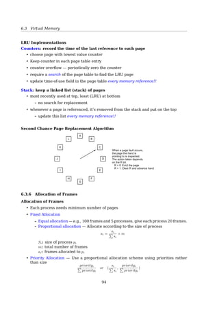
93. 6.3 Virtual Memory
• Improved I/O performance — much
faster than read() and write() system
calls
• Lazy loading (demand paging) — only a
small portion of file is loaded initially
• A mapped file can be shared, like
shared library
virtual memory and can be seen by all others that map the same section of
the file. Given our earlier discussions of virtual memory, it should be clear
how the sharing of memory-mapped sections of memory is implemented:
the virtual memory map of each sharing process points to the same page of
physical memory—the page that holds a copy of the disk block. This memory
sharing is illustrated in Figure 8.23. The memory-mapping system calls can
also support copy-on-write functionality, allowing processes to share a file in
read-only mode but to have their own copies of any data they modify. So that
process A
virtual memory
1
1
1 2 3 4 5 6
2
3
3
4
5
5
4
2
6
6
1
2
3
4
5
6
process B
virtual memory
physical memory
disk file
Figure 8.23 Memory-mapped files.
6.3.5 Page Replacement Algorithms
Need For Page Replacement
Page replacement: find some page in memory, but not really in use, swap it out332 Chapter 8 Virtual Memory
monitor
load M
physical
memory
1
0
2
3
4
5
6
7
H
load M
J
M
logical memory
for user 1
0
PC
1
2
3 B
M
valid–invalid
bitframe
page table
for user 1
i
A
B
D
E
logical memory
for user 2
0
1
2
3
valid–invalid
bitframe
page table
for user 2
i
4
3
5
v
v
v
7
2 v
v
6 v
D
H
J
A
E
Figure 8.9 Need for page replacement.
Over-allocation of memory manifests itself as follows. While a user process
is executing, a page fault occurs. The operating system determines where the
desired page is residing on the disk but then finds that there are no free frames
on the free-frame list; all memory is in use (Figure 8.9).
The operating system has several options at this point. It could terminate
the user process. However, demand paging is the operating system’s attempt to
improve the computer system’s utilization and throughput. Users should not
be aware that their processes are running on a paged system—paging should
be logically transparent to the user. So this option is not the best choice.
The operating system could instead swap out a process, freeing all its
frames and reducing the level of multiprogramming. This option is a good one
in certain circumstances, and we consider it further in Section 8.6. Here, we
discuss the most common solution: page replacement.
8.4.1 Basic Page Replacement
Page replacement takes the following approach. If no frame is free, we find
one that is not currently being used and free it. We can free a frame by writing
its contents to swap space and changing the page table (and all other tables) to
indicate that the page is no longer in memory (Figure 8.10). We can now use
the freed frame to hold the page for which the process faulted. We modify the
page-fault service routine to include page replacement:
1. Find the location of the desired page on the disk.
2. Find a free frame:
a. If there is a free frame, use it.
Linux calls it the Page Frame Reclaiming Algorithm10
, it’s basically LRU with a bias
towards non-dirty pages.
See also
• [33, Page replacement algorithm]
• [2, Chap. 17, Page Frame Reclaiming].
• PageReplacementDesign11
10http://stackoverflow.com/questions/5889825/page-replacement-algorithm
11http://linux-mm.org/PageReplacementDesign
93

94. 6.3 Virtual Memory
Performance Concern
Because disk I/O is so expensive, we must solve two major problems to implement
demand paging.
Frame-allocation algorithm If we have multiple processes in memory, we must decide
how many frames to allocate to each process.
Page-replacement algorithm When page replacement is required, we must select the
frames that are to be replaced.
Performance
We want an algorithm resulting in lowest page-fault rate
• Is the victim page modified?
• Pick a random page to swap out?
• Pick a page from the faulting process’ own pages? Or from others?
Page-Fault Frequency Scheme
Establish ”acceptable” page-fault rate
FIFO Page Replacement Algorithm
• Maintain a linked list (FIFO queue) of all pages
– in order they came into memory
• Page at beginning of list replaced
• Disadvantage
– The oldest page may be often used
– Belady’s anomaly
94

95. 6.3 Virtual Memory
FIFO Page Replacement Algorithm
Belady’s Anomaly
• Reference string: 1, 2, 3, 4, 1, 2, 5, 1, 2, 3, 4, 5
• 3 frames (3 pages can be in memory at a time per process)
1 4 5 3
2 1 /1 4
3 2 /2 /5
9 page faults
• 4 frames
1 /1 2
2 /2 3
3 5 4
4 1 5
10 page faults
• Belady’s Anomaly: more frames ⇒ more page faults
Optimal Page Replacement Algorithm (OPT)
• Replace page needed at the farthest point in future
– Optimal but not feasible
• Estimate by ...
– logging page use on previous runs of process
– although this is impractical, similar to SJF CPU-scheduling, it can be used for
comparison studies
Least Recently Used (LRU) Algorithm
FIFO uses the time when a page was brought into memory
OPT uses the time when a page is to be used
LRU uses the recent past as an approximation of the near future
Assume recently-used-pages will used again soon
replace the page that has not been used for the longest period of time
95

96. 6.3 Virtual Memory
LRU Implementations
Counters: record the time of the last reference to each page
• choose page with lowest value counter
• Keep counter in each page table entry
• counter overflow — periodically zero the counter
• require a search of the page table to find the LRU page
• update time-of-use field in the page table every memory reference!
Stack: keep a linked list (stack) of pages
• most recently used at top, least (LRU) at bottom
– no search for replacement
• whenever a page is referenced, it’s removed from the stack and put on the top
– update this list every memory reference!
Second Chance Page Replacement Algorithm
When a page fault occurs,
the page the hand is
pointing to is inspected.
The action taken depends
on the R bit:
R = 0: Evict the page
R = 1: Clear R and advance hand
A
B
C
D
E
F
G
H
I
J
K
L
Fig. 4-17. The clock page replacement algorithm.6.3.6 Allocation of Frames
Allocation of Frames
• Each process needs minimum number of pages
• Fixed Allocation
96

97. 6.3 Virtual Memory
– Equal allocation — e.g., 100 frames and 5 processes, give each process 20 frames.
– Proportional allocation — Allocate according to the size of process
ai =
si
∑
si
× m
Si: size of process pi
m: total number of frames
ai: frames allocated to pi
• Priority Allocation — Use a proportional allocation scheme using priorities rather
than size
priorityi
∑
priorityi
or (
si
∑
si
,
priorityi
∑
priorityi
)
Global vs. Local Allocation
If process Pi generates a page fault, it can select a replacement frame
• from its own frames — Local replacement
• from the set of all frames; one process can take a frame from another — Global re-
placement
– from a process with lower priority number
Global replacement generally results in greater system throughput.
6.3.7 Thrashing And Working Set Model
Thrashing 8.6 Thrashing 349
thrashing
degree of multiprogramming
CPUutilization
Figure 8.18 Thrashing.
thrashing, they will be in the queue for the paging device most of the time. The
average service time for a page fault will increase because of the longer average
queue for the paging device. Thus, the effective access time will increase even
for a process that is not thrashing.
To prevent thrashing, we must provide a process with as many frames as
it needs. But how do we know how many frames it “needs”? There are several
techniques. The working-set strategy (Section 8.6.2) starts by looking at how
many frames a process is actually using. This approach defines the locality
model of process execution.
The locality model states that, as a process executes, it moves from locality
to locality. A locality is a set of pages that are actively used together (Figure
8.19). A program is generally composed of several different localities that may
overlap.
For example, when a function is called, it defines a new locality. In this
locality, memory references are made to the instructions of the function call, its
local variables, and a subset of the global variables. When we exit the function,
the process leaves this locality, since the local variables and instructions of the
function are no longer in active use. We may return to this locality later.
Thus, we see that localities are defined by the program structure and its
data structures. The locality model states that all programs will exhibit this
basic memory reference structure. Note that the locality model is the unstated
principle behind the caching discussions so far in this book. If accesses to any
types of data were random rather than patterned, caching would be useless.
Suppose we allocate enough frames to a process to accommodate its current
locality. It will fault for the pages in its locality until all these pages are in
memory; then, it will not fault again until it changes localities. If we do not
allocate enough frames to accommodate the size of the current locality, the
process will thrash, since it cannot keep in memory all the pages that it is
actively using.
Thrashing
1. CPU not busy ⇒ add more processes
2. a process needs more frames ⇒ faulting, and taking frames away from others
3. these processes also need these pages ⇒ also faulting, and taking frames away from
others ⇒ chain reaction
4. more and more processes queueing for the paging device ⇒ ready queue is empty ⇒
CPU has nothing to do ⇒ add more processes ⇒ more page faults
5. MMU is busy, but no work is getting done, because processes are busy paging —
thrashing
97

98. 6.3 Virtual Memory
Demand Paging and Thrashing
Locality Model
• A locality is a set of pages that are ac-
tively used together
• Process migrates from one locality to
another
350 Chapter 8 Virtual Memory
18
20
22
24
26
28
30
32
34
pagenumbersmemoryaddress
execution time
Figure 8.19 Locality in a memory-reference pattern.
is to examine the most recent page references. The set of pages in the most
recent page references is the working set (Figure 8.20). If a page is in active
use, it will be in the working set. If it is no longer being used, it will drop from
the working set time units after its last reference. Thus, the working set is an
approximation of the program’s locality.
For example, given the sequence of memory references shown in Figure
8.20, if = 10 memory references, then the working set at time t1 is {1, 2, 5,
6, 7}. By time t2, the working set has changed to {3, 4}.
The accuracy of the working set depends on the selection of . If is too
small, it will not encompass the entire locality; if is too large, it may overlap
locality in a memory reference pattern
Why does thrashing occur?
∑
i=(0,n)
Localityi total memory size
Working-Set Model
Working Set (WS) The set of pages that a process is currently(∆) using. (≈ locality)8.6 Thrashing 351
page reference table
. . . 2 6 1 5 7 7 7 7 5 1 6 2 3 4 1 2 3 4 4 4 3 4 3 4 4 4 1 3 2 3 4 4 4 3 4 4 4 . . .
Δ
t1
WS(t1
) = {1,2,5,6,7}
Δ
t2
WS(t2
) = {3,4}
Figure 8.20 Working-set model.
several localities. In the extreme, if is infinite, the working set is the set of
pages touched during the process execution.
The most important property of the working set, then, is its size. If we
compute the working-set size, WSSi , for each process in the system, we can
then consider that
D = WSSi ,
where D is the total demand for frames. Each process is actively using the pages
in its working set. Thus, process i needs WSSi frames. If the total demand is
greater than the total number of available frames (D m), thrashing will occur,
because some processes will not have enough frames.
Once has been selected, use of the working-set model is simple. The
operating system monitors the working set of each process and allocates to
that working set enough frames to provide it with its working-set size. If there
are enough extra frames, another process can be initiated. If the sum of the
working-set sizes increases, exceeding the total number of available frames,
the operating system selects a process to suspend. The process’s pages are
written out (swapped), and its frames are reallocated to other processes. The
suspended process can be restarted later.
This working-set strategy prevents thrashing while keeping the degree of
multiprogramming as high as possible. Thus, it optimizes CPU utilization.
The difficulty with the working-set model is keeping track of the working
set. The working-set window is a moving window. At each memory reference,
∆: Working-set window. In this example,
∆ = 10 memory access
WSS: Working-set size. WS(t1) = {
W SS=5
1, 2, 5, 6, 7}
• The accuracy of the working set depends on the selection of ∆
• Thrashing, if
∑
WSSi SIZEtotal memory
98

99. 6.3 Virtual Memory
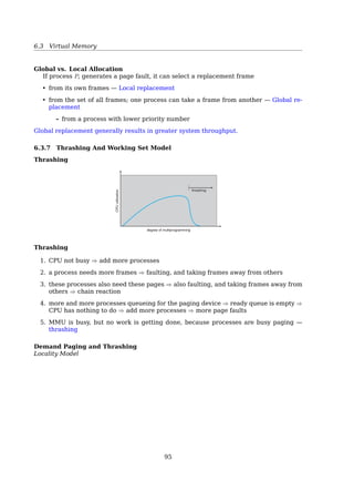
The Working-Set Page Replacement Algorithm
To evict a page that is not in the working set
Information about
one page 2084
2204 Current virtual time
2003
1980
1213
2014
2020
2032
1620
Page table
1
1
1
0
1
1
1
0
Time of last use
Page referenced
during this tick
Page not referenced
during this tick
R (Referenced) bit
Scan all pages examining R bit:
if (R == 1)
set time of last use to current virtual time
if (R == 0 and age τ)
remove this page
if (R == 0 and age ≤ τ)
remember the smallest time
Fig. 4-21. The working set algorithm.
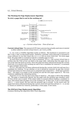
age = Current virtual time − Time of last use
Current virtual time The amount of CPU time a process has actually used since it started
is often called its current virtual time [19, sec 3.4.8, p 209].
The algorithm works as follows. The hardware is assumed to set the R and M bits, as
discussed earlier. Similarly, a periodic clock interrupt is assumed to cause software to run
that clears the Referenced bit on every clock tick. On every page fault, the page table is
scanned to look for a suitable page to evict[19, sec 3.4.8, p 210].
As each entry is processed, the R bit is examined. If it is 1, the current virtual time is
written into the Time of last use field in the page table, indicating that the page was in
use at the time the fault occurred. Since the page has been referenced during the current
clock tick, it is clearly in the working set and is not a candidate for removal (τ is assumed
to span multiple clock ticks).
If R is 0, the page has not been referenced during the current clock tick and may be a
candidate for removal. To see whether or not it should be removed, its age (the current
virtual time minus its Time of last use) is computed and compared to τ. If the age is greater
than τ, the page is no longer in the working set and the new page replaces it. The scan
continues updating the remaining entries.
However, if R is 0 but the age is less than or equal to τ, the page is still in the working
set. The page is temporarily spared, but the page with the greatest age (smallest value
of Time of last use) is noted. If the entire table is scanned without finding a candidate
to evict, that means that all pages are in the working set. In that case, if one or more
pages with R = 0 were found, the one with the greatest age is evicted. In the worst case,
all pages have been referenced during the current clock tick (and thus all have R = 1), so
one is chosen at random for removal, preferably a clean page, if one exists.
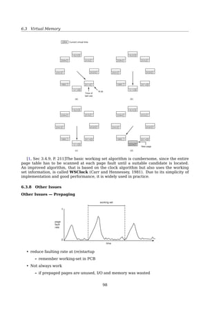
The WSClock Page Replacement Algorithm
Combine Working Set Algorithm With Clock Algorithm
99

100. 6.3 Virtual Memory
2204 Current virtual time
1213 0
2084 1 2032 1
1620 0
2020 12003 1
1980 1 2014 1
Time of
last use
R bit
(a) (b)
(c) (d)
New page
1213 0
2084 1 2032 1
1620 0
2020 12003 1
1980 1 2014 0
1213 0
2084 1 2032 1
1620 0
2020 12003 1
1980 1 2014 0
2204 1
2084 1 2032 1
1620 0
2020 12003 1
1980 1 2014 0
Fig. 4-22. Operation of the WSClock algorithm. (a) and (b) give
an example of what happens when R = 1. (c) and (d) give an
example of R = 0.
The basic working set algorithm is cumbersome, since the entire page table has to be
scanned at each page fault until a suitable candidate is located. An improved algorithm,
that is based on the clock algorithm but also uses the working set information, is called
WSClock (Carr and Hennessey, 1981). Due to its simplicity of implementation and good
performance, it is widely used in practice[19, Sec 3.4.9, P. 211].
6.3.8 Other Issues
Other Issues — Prepaging
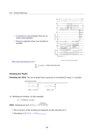
8.7 Memory-Mapped Files 353
WORKING SETS AND PAGE FAULT RATES
There is a direct relationship between the working set of a process and its
page-fault rate. Typically, as shown in Figure 8.20, the working set of a process
changes over time as references to data and code sections move from one
locality to another. Assuming there is sufficient memory to store the working
set of a process (that is, the process is not thrashing), the page-fault rate of
the process will transition between peaks and valleys over time. This general
behavior is shown in Figure 8.22.
1
0
time
working set
page
fault
rate
Figure 8.22 Page fault rate over time.
A peak in the page-fault rate occurs when we begin demand-paging a new
locality. However, once the working set of this new locality is in memory,
the page-fault rate falls. When the process moves to a new working set, the
page-fault rate rises toward a peak once again, returning to a lower rate once
the new working set is loaded into memory. The span of time between the
start of one peak and the start of the next peak represents the transition from
one working set to another.
8.7.1 Basic Mechanism
Memory mapping a file is accomplished by mapping a disk block to a page (or
pages) in memory. Initial access to the file proceeds through ordinary demand
• reduce faulting rate at (re)startup
– remember working-set in PCB
• Not always work
– if prepaged pages are unused, I/O and memory was wasted
100

101. 6.3 Virtual Memory
Other Issues — Page Size
Larger page size
« Bigger internal fragmentation
« longer I/O time
Smaller page size
« Larger page table
« more page faults
– one page fault for each byte, if page size = 1 Byte
– for a 200K process, with page size = 200K, only one page fault
No best answer
$ getconf PAGESIZE
Other Issues — TLB Reach
• Ideally, the working set of each process is stored in the TLB
– Otherwise there is a high degree of page faults
• TLB Reach — The amount of memory accessible from the TLB
TLB Reach = (TLB Size) × (Page Size)
• Increase the page size
Internal fragmentation may be increased
• Provide multiple page sizes
– This allows applications that require larger page sizes the opportunity to use
them without an increase in fragmentation
* UltraSPARC supports page sizes of 8KB, 64KB, 512KB, and 4MB
* Pentium supports page sizes of 4KB and 4MB
Other Issues — Program Structure
Careful selection of data structures and programming structures can increase locality,
i.e. lower the page-fault rate and the number of pages in the working set.
Example
• A stack has a good locality, since access is always made to the top
• A hash table has a bad locality, since it’s designed to scatter references
• Programming language
– Pointers tend to randomize access to memory
– OO programs tend to have a poor locality
101

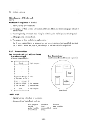
102. 6.3 Virtual Memory
Other Issues — Program Structure
Example
• int[i][j] = int[128][128]
• Assuming page size is 128 words, then
• Each row (128 words) takes one page
If the process has fewer than 128 frames
Program 1:
for(j=0;j128;j++)
for(i=0;i128;i++)
data[i][j] = 0;
Worst case:
128 × 128 = 16, 384 page faults
Program 2:
for(i=0;i128;i++)
for(j=0;j128;j++)
data[i][j] = 0;
Worst case:
128 page faults
See also: [17, Sec. 8.9.5, Program Structure]
Other Issues — I/O interlock
Sometimes it is necessary to lock pages in memory so that they are not paged out.
Example
• The OS
• I/O operation — the frame into which the I/O device was scheduled to write should
not be replaced.
• New page that was just brought in — looks like the best candidate to be replaced
because it was not accessed yet, nor was it modified.
Other Issues — I/O interlock
Case 1
Be sure the following sequence of events does not occur:
1. A process issues an I/O request, and then queueing for that I/O device
2. The CPU is given to other processes
3. These processes cause page faults
4. The waiting process’ page is unluckily replaced
5. When its I/O request is served, the specific frame is now being used by another pro-
cess
102

103. 6.3 Virtual Memory
Other Issues — I/O interlock
Case 2
Another bad sequence of events:
1. A low-priority process faults
2. The paging system selects a replacement frame. Then, the necessary page is loaded
into memory
3. The low-priority process is now ready to continue, and waiting in the ready queue
4. A high-priority process faults
5. The paging system looks for a replacement
(a) It sees a page that is in memory but not been referenced nor modified: perfect!
(b) It doesn’t know the page is just brought in for the low-priority process
6.3.9 Segmentation
Two Views of A Virtual Address Space
One-dimensional
a linear array of bytes
max +------------------+
| Stack | Stack segment
+--------+---------+
| | |
| v |
| |
| ^ |
| | |
+--------+---------+
| Dynamic storage | Heap
|(from new, malloc)|
+------------------+
| Static variables |
| (uninitialized, | BSS segment
| initialized) | Data segment
+------------------+
| Code | Text segment
0 +------------------+
Two-dimensional
a collection of variable-sized segments
User’s View
• A program is a collection of segments
• A segment is a logical unit such as:
main program procedure function
method object local variables
global variables common block stack
symbol table arrays
103

104. 6.3 Virtual Memory
Logical And Physical View of Segmentation
8.46 Silberschatz, Galvin and Gagne ©2009Operating System Concepts – 8th Edition
Logical View of Segmentation
1
3
2
4
1
4
2
3
user space physical memory space
«
Segmentation Architecture
• Logical address consists of a two tuple:
segment-number, offset
• Segment table maps 2D virtual addresses into 1D physical addresses; each table entry
has:
– base contains the starting physical address where the segments reside in memory
– limit specifies the length of the segment
• Segment-table base register (STBR) points to the segment table’s location in memory
• Segment-table length register (STLR) indicates number of segments used by a pro-
gram;
segment number s is legal if s STLR
Segmentation hardware306 Chapter 7 Main Memory
CPU
physical memory
s d
+
trap: addressing error
no
yes
segment
table
limit base
s
Figure 7.19 Segmentation hardware.
Libraries that are linked in during compile time might be assigned separate
segments. The loader would take all these segments and assign them segment
numbers.
7.6.2 Hardware
Although the user can now refer to objects in the program by a two-dimensional
address, the actual physical memory is still, of course, a one-dimensional
104

105. 6.3 Virtual Memory
7.7 Example: The Intel Pentium 307
logical address space
subroutine stack
symbol
table
main
program
Sqrt
1400
physical memory
2400
3200
segment 2
4300
4700
5700
6300
6700
segment table
limit
0
1
2
3
4
1000
400
400
1100
1000
base
1400
6300
4300
3200
4700
segment 0
segment 3
segment 4
segment 2segment 1
segment 0
segment 3
segment 4
segment 1
Figure 7.20 Example of segmentation.
onto location 4300 + 53 = 4353. A reference to segment 3, byte 852, is mapped to
3200 (the base of segment 3) + 852 = 4052. A reference to byte 1222 of segment
0 would result in a trap to the operating system, as this segment is only 1,000
bytes long.
7.7 Example: The Intel Pentium
Both paging and segmentation have advantages and disadvantages. In fact,
some architectures provide both. In this section, we discuss the Intel Pentium
architecture, which supports both pure segmentation and segmentation with
paging. We do not give a complete description of the memory-management
structure of the Pentium in this text. Rather, we present the major ideas on
which it is based. We conclude our discussion with an overview of Linux
address translation on Pentium systems.
In Pentium systems, the CPU generates logical addresses, which are given
to the segmentation unit. The segmentation unit produces a linear address for
each logical address. The linear address is then given to the paging unit, which
in turn generates the physical address in main memory. Thus, the segmentation
and paging units form the equivalent of the memory-management unit (MMU).
This scheme is shown in Figure 7.21.
7.7.1 Pentium Segmentation
The Pentium architecture allows a segment to be as large as 4 GB, and the
maximum number of segments per process is 16 K. The logical-address space
(0, 1222) ⇒ Trap!
(3, 852) ⇒ 3200 + 852 = 4052
(2, 53) ⇒ 4300 + 53 = 4353
Advantages of Segmentation
• Each segment can be
– located independently
– separately protected
– grow independently
• Segments can be shared between processes
Problems with Segmentation
• Variable allocation
• Difficult to find holes in physical memory
• Must use one of non-trivial placement algorithm
– first fit, best fit, worst fit
• External fragmentation
See also: http://cseweb.ucsd.edu/classes/fa03/cse120/Lec08.pdf
Linux prefers paging to segmentation
Because
• Segmentation and paging are somewhat redundant
105

106. 6.3 Virtual Memory
• Memory management is simpler when all processes share the same set of linear ad-
dresses
• Maximum portability. RISC architectures in particular have limited support for seg-
mentation
The Linux 2.6 uses segmentation only when required by the 80x86 architecture.
Case Study: The Intel Pentium
Segmentation With Paging
|--------------- MMU ---------------|
+--------------+ +--------+ +----------+
+-----+ Logical | Segmentation | Linear | Paging | Physical | Physical |
| CPU |----------| unit |----------| unit |-----------| memory |
+-----+ address +--------------+ address +--------+ address +----------+
selector | offset
+----+---+---+--------+
| s | g | p | |
+----+---+---+--------+
13 1 2 32
page number | page offset
+----------+----------+------------+
| p1 | p2 | d |
+----------+----------+------------+
10 10 12
| |
| ‘- pointing to 1k frames
‘-- pointing to 1k page tables
Segmentation
Logical Address ⇒ Linear Address
106

107. 6.3 Virtual Memory
7.7 Example: The Intel Pentium 309
logical address selector
descriptor table
segment descriptor +
32-bit linear address
offset
Figure 7.22 Intel Pentium segmentation.
detail in Figure 7.23. The 10 high-order bits reference an entry in the outermost
page table, which the Pentium terms the page directory. (The CR3 register
points to the page directory for the current process.) The page directory entry
points to an inner page table that is indexed by the contents of the innermost
10 bits in the linear address. Finally, the low-order bits 0–11 refer to the offset
in the 4-KB page pointed to in the page table.
One entry in the page directory is the Page Size flag, which—if set—
indicates that the size of the page frame is 4 MB and not the standard 4 KB.
If this flag is set, the page directory points directly to the 4-MB page frame,
bypassing the inner page table; and the 22 low-order bits in the linear address
refer to the offset in the 4-MB page frame.
page directory
page directory
CR3
register
page
directory
page
table
4-KB
page
4-MB
page
page table
offset
offset
(linear address)
31 22 21 12 11 0
2131 22 0
Figure 7.23 Paging in the Pentium architecture.
Segment Selectors
A logical address consists of two parts:
segment selector : offset
16 bits 32 bits
Segment selector is an index into GDT/LDT
selector | offset
+-----+-+--+--------+ s - segment number
| s |g|p | | g - 0-global; 1-local
+-----+-+--+--------+ p - protection use
13 1 2 32
Segment Descriptor Tables
All the segments are organized in 2 tables:
GDT Global Descriptor Table
• shared by all processes
• GDTR stores address and size of the GDT
LDT Local Descriptor Table
• one process each
• LDTR stores address and size of the LDT
Segment descriptors are entries in either GDT or LDT, 8-byte long
Analogy
Process ⇐⇒ Process Descriptor(PCB)
File ⇐⇒ Inode
Segment ⇐⇒ Segment Descriptor
See also:
• Memory Tanslation And Segmentation12
12http://duartes.org/gustavo/blog/post/memory-translation-and-segmentation
107

108. 6.3 Virtual Memory
• The GDT13
• The GDT and IDT14
Segment Registers
The Intel Pentium has
• 6 segment registers, allowing 6 segments to be addressed at any one time by a pro-
cess
– Each segment register

109. an entry in LDT/GDT
• 6 8-byte micro program registers to hold descriptors from either LDT or GDT
– avoid having to read the descriptor from memory for every memory reference
0 1 2 3~8 9
+--------+--------|--------+---//---+--------+
| Segment selector| Micro program register |
+--------+--------|--------+---//---+--------+
Programmable Non-programmable
Fast access to segment descriptors
An additional nonprogrammable register for each segment register
DESCRIPTOR TABLE SEGMENT
+--------------+ +------+
| ... | ,-------| |--.
+--------------+ | | | |
.---| Segment |____/ | | |
| | Descriptor | +------+ |
| +--------------+ |
| | ... | |
| +--------------+ |
| Nonprogrammable |
| Segment Registor Register |
__+------------------+--------------------+____/
| Segment Selector | Segment Descriptor |
+------------------+--------------------+
Segment registers hold segment selectors
cs code segment register
CPL 2-bit, specifies the Current Privilege Level of the CPU
00 - Kernel mode
11 - User mode
ss stack segment register
ds data segment register
13http://www.osdever.net/bkerndev/Docs/gdt.htm
14http://www.jamesmolloy.co.uk/tutorial_html/4.-The%20GDT%20and%20IDT.html
108

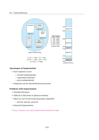
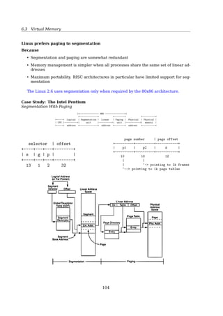
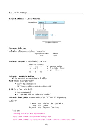
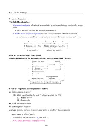
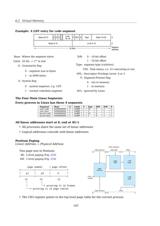
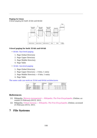
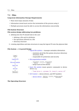
110. 6.3 Virtual Memory
es/fs/gs general purpose registers, may refer to arbitrary data segments
See also:
• [9, Sec. 6.3.2, Restricting Access to Data].
• CPU Rings, Privilege, and Proctection15
Example: A LDT entry for code segment
Privilege level (0-3)
Relative
address
0
4
Base 0-15 Limit 0-15
Base 24-31 Base 16-23
Limit
16-19
G D 0 P DPL Type
0: Li is in bytes
1: Li is in pages
0: 16-Bit segment
1: 32-Bit segment
0: Segment is absent from memory
1: Segment is present in memory
Segment type and protection
S
;; 0: System
1: Application
32 Bits
Fig. 4-44. Pentium code segment descriptor. Data segments differ
slightly.
Base: Where the segment starts
Limit: 20 bit, ⇒ 220
in size
G: Granularity flag
0 - segment size in bytes
1 - in 4096 bytes
S: System flag
0 - system segment, e.g. LDT
1 - normal code/data segment
D/B: 0 - 16-bit offset
1 - 32-bit offset
Type: segment type (cs/ds/tss)
TSS: Task status, i.e. it’s executing or not
DPL: Descriptor Privilege Level. 0 or 3
P: Segment-Present flag
0 - not in memory
1 - in memory
AVL: ignored by Linux
The Four Main Linux Segments
Every process in Linux has these 4 segments
Segment Base G Limit S Type DPL D/B P
user code 0x00000000 1 0xfffff 1 10 3 1 1
user data 0x00000000 1 0xfffff 1 2 3 1 1
kernel code 0x00000000 1 0xfffff 1 10 0 1 1
kernel data 0x00000000 1 0xfffff 1 2 0 1 1
All linear addresses start at 0, end at 4G-1
• All processes share the same set of linear addresses
• Logical addresses coincide with linear addresses
Pentium Paging
Linear Address ⇒ Physical Address
15http://duartes.org/gustavo/blog/post/cpu-rings-privilege-and-protection
109

111. 6.3 Virtual Memory
Two page size in Pentium:
4K: 2-level paging (Fig. 219)
4M: 1-level paging (Fig. 214)
page number | page offset
+----------+----------+------------+
| p1 | p2 | d |
+----------+----------+------------+
10 10 12
| |
| ‘- pointing to 1k frames
‘-- pointing to 1k page tables
points to the page directory for the current process.) The page directory entry
points to an inner page table that is indexed by the contents of the innermost
10 bits in the linear address. Finally, the low-order bits 0–11 refer to the offset
in the 4-KB page pointed to in the page table.
One entry in the page directory is the Page Size flag, which—if set—
indicates that the size of the page frame is 4 MB and not the standard 4 KB.
If this flag is set, the page directory points directly to the 4-MB page frame,
bypassing the inner page table; and the 22 low-order bits in the linear address
refer to the offset in the 4-MB page frame.
page directory
page directory
CR3
register
page
directory
page
table
4-KB
page
4-MB
page
page table
offset
offset
(linear address)
31 22 21 12 11 0
2131 22 0
Figure 7.23 Paging in the Pentium architecture.
• The CR3 register points to the top level page table for the current process.
Paging In Linux
4-level paging for both 32-bit and 64-bit
Global directory Upper directory Middle directory Page Offset
Page
Page table
Page middle
directory
Page upper
directory
Page global
directory
Virtual
address
cr3
4-level paging for both 32-bit and 64-bit
• 64-bit: four-level paging
1. Page Global Directory
2. Page Upper Directory
3. Page Middle Directory
4. Page Table
• 32-bit: two-level paging
1. Page Global Directory
2. Page Upper Directory — 0 bits; 1 entry
3. Page Middle Directory — 0 bits; 1 entry
4. Page Table
The same code can work on 32-bit and 64-bit architectures
Page Address Paging Address
Arch size bits levels splitting
x86 4KB(12bits) 32 2 10 + 0 + 0 + 10 + 12
x86-PAE 4KB(12bits) 32 3 2 + 0 + 9 + 9 + 12
x86-64 4KB(12bits) 48 4 9 + 9 + 9 + 9 + 12
110

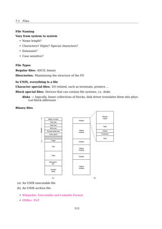
112. References
[1] Wikipedia. Memory management — Wikipedia, The Free Encyclopedia. [Online; ac-
cessed 21-February-2015]. 2015.
[2] Wikipedia. Virtual memory — Wikipedia, The Free Encyclopedia. [Online; accessed
21-February-2015]. 2015.
7 File Systems
7.1 File System Structure
Long-term Information Storage Requirements
• Must store large amounts of data
• Information stored must survive the termination of the process using it
• Multiple processes must be able to access the information concurrently
File-System Structure
File-system design addressing two problems:
1. defining how the FS should look to the user
• defining a file and its attributes
• the operations allowed on a file
• directory structure
2. creating algorithms and data structures to map the logical FS onto the physical disk
File-System — A Layered Design
APPs
⇓
Logical FS
⇓
File-org module
⇓
Basic FS
⇓
I/O ctrl
⇓
Devices
• logical file system — manages metadata information
- maintains all of the file-system structure (directory struc-
ture, FCB)
- responsible for protection and security
• file-organization module
- logical block
address
translate
−−−−−−→ physical block
address
- keeps track of free blocks
• basic file system issues generic commands to device driver, e.g
- “read drive 1, cylinder 72, track 2, sector 10”
• I/O Control — device drivers, and INT handlers
- device driver: high-level
commands
translate
−−−−−−→ hardware-specific
instructions
See also [19, Sec. 1.3.5, I/O Devices].
111

113. 7.2 Files
The Operating Structure
APPs
⇓
Logical FS
⇓
File-org module
⇓
Basic FS
⇓
I/O ctrl
⇓
Devices
Example — To create a file
1. APP calls creat()
2. Logical FS
(a) allocates a new FCB
(b) updates the in-mem dir structure
(c) writes it back to disk
(d) calls the file-org module
3. file-organization module
(a) allocates blocks for storing the file’s data
(b) maps the directory I/O into disk-block numbers
Benefit of layered design
The I/O control and sometimes the basic file system code can be used by multiple file
systems.
7.2 Files
File
A Logical View Of Information Storage
User’s view
A file is the smallest storage unit on disk.
– Data cannot be written to disk unless they are within a file
UNIX view
Each file is a sequence of 8-bit bytes
– It’s up to the application program to interpret this byte stream.
File
What Is Stored In A File?
Source code, object files, executable files, shell scripts, PostScript...
Different type of files have different structure
• UNIX looks at contents to determine type
Shell scripts start with “#!”
PDF start with “%PDF...”
Executables start with magic number
• Windows uses file naming conventions
executables end with “.exe” and “.com”
MS-Word end with “.doc”
MS-Excel end with “.xls”
112

114. 7.2 Files
File Naming
Vary from system to system
• Name length?
• Characters? Digits? Special characters?
• Extension?
• Case sensitive?
File Types
Regular files: ASCII, binary
Directories: Maintaining the structure of the FS
In UNIX, everything is a file
Character special files: I/O related, such as terminals, printers ...
Block special files: Devices that can contain file systems, i.e. disks
disks — logically, linear collections of blocks; disk driver translates them into phys-
ical block addresses
Binary files
(a) (b)
Header
Header
Header
Magic number
Text size
Data size
BSS size
Symbol table size
Entry point
Flags
Text
Data
Relocation
bits
Symbol
table
Object
module
Object
module
Object
module
Module
name
Date
Owner
Protection
Size
;
;;
Header
Fig. 6-3. (a) An executable file. (b) An archive.
(a) An UNIX executable file
(b) An UNIX archive file
113

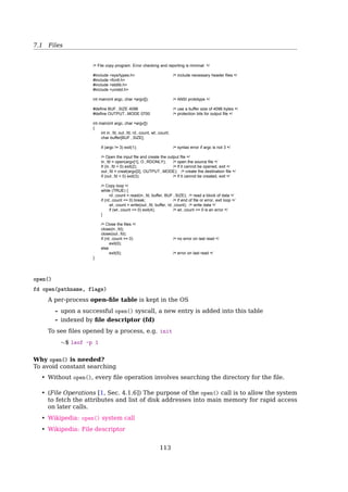
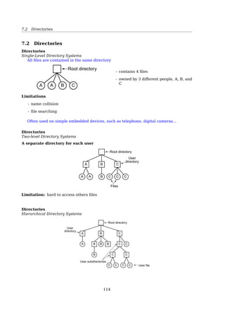
115. 7.2 Files
See also:
• [26, Executable and Linkable Format]
• OSDev: ELF16
File Attributes — Metadata
• Name only information kept in human-readable form
• Identifier unique tag (number) identifies file within file system
• Type needed for systems that support different types
• Location pointer to file location on device
• Size current file size
• Protection controls who can do reading, writing, executing
• Time, date, and user identification data for protection, security, and usage monitor-
ing
File Operations
POSIX file system calls
1. fd = creat(name, mode)
2. fd = open(name, flags)
3. status = close(fd)
4. byte_count = read(fd, buffer, byte_count)
5. byte_count = write(fd, buffer, byte_count)
6. offset = lseek(fd, offset, whence)
7. status = link(oldname, newname)
8. status = unlink(name)
9. status = truncate(name, size)
10. status = ftruncate(fd, size)
11. status = stat(name, buffer)
12. status = fstat(fd, buffer)
13. status = utimes(name, times)
14. status = chown(name, owner, group)
15. status = fchown(fd, owner, group)
16. status = chmod(name, mode)
17. status = fchmod(fd, mode)
16http://wiki.osdev.org/ELF
114

116. 7.2 Files
An Example Program Using File System Calls
/* File copy program. Error checking and reporting is minimal. */
#include sys/types.h /* include necessary header files */
#include fcntl.h
#include stdlib.h
#include unistd.h
int main(int argc, char *argv[]); /* ANSI prototype */
#define BUF SIZE 4096 /* use a buffer size of 4096 bytes */
#define OUTPUT MODE 0700 /* protection bits for output file */
int main(int argc, char *argv[])
{
int in fd, out fd, rd count, wt count;
char buffer[BUF SIZE];
if (argc != 3) exit(1); /* syntax error if argc is not 3 */
/* Open the input file and create the output file */
in fd = open(argv[1], O RDONLY); /* open the source file */
if (in fd 0) exit(2); /* if it cannot be opened, exit */
out fd = creat(argv[2], OUTPUT MODE); /* create the destination file */
if (out fd 0) exit(3); /* if it cannot be created, exit */
/* Copy loop */
while (TRUE) {
rd count = read(in fd, buffer, BUF SIZE); /* read a block of data */
if (rd count = 0) break; /* if end of file or error, exit loop */
wt count = write(out fd, buffer, rd count); /* write data */
if (wt count = 0) exit(4); /* wt count = 0 is an error */
}
/* Close the files */
close(in fd);
close(out fd);
if (rd count == 0) /* no error on last read */
exit(0);
else
exit(5); /* error on last read */
}
Fig. 6-5. A simple program to copy a file.open()
fd open(pathname, flags)
A per-process open-file table is kept in the OS
– upon a successful open() syscall, a new entry is added into this table
– indexed by file descriptor (fd)
To see files opened by a process, e.g. init
$ lsof -p 1
Why open() is needed?
To avoid constant searching
• Without open(), every file operation involves searching the directory for the file.
The purpose of the open() call is to allow the system to fetch the attributes and list
of disk addresses into main memory for rapid access on later calls [19, Sec. 4.1.6, File
Operations].
See also:
• [32, open() system call]
• [28, File descriptor]
115

117. 7.3 Directories
7.3 Directories
Directories
Single-Level Directory Systems
All files are contained in the same directory
Root directory
A A B C
Fig. 6-7. A single-level directory system containing four files,
owned by three different people, A, B, and C.
- contains 4 files
- owned by 3 different people, A, B, and
C
Limitations
- name collision
- file searching
Often used on simple embedded devices, such as telephone, digital cameras...
Directories
Two-level Directory Systems
A separate directory for each user
Files
User
directory
A A
A B
B
C
CC C
Root directory
Fig. 6-8. A two-level directory system. The letters indicate the
owners of the directories and files.
Limitation: hard to access others files
Directories
Hierarchical Directory Systems
User
directory
User subdirectories
C C
C
C C
C
B
B
A
A
B
B
C C
C
B
Root directory
User file
Fig. 6-9. A hierarchical directory system.
116

118. 7.4 File System Implementation
Directories
Path Names
ROOT
bin boot dev etc home var
grub passwd staff stud mail
w x 6 7 2 20081152001
dir
file
20081152001
Directories
Directory Operations
Create Delete Rename Link
Opendir Closedir Readdir Unlink
7.4 File System Implementation
7.4.1 Basic Structures
File System Implementation
A typical file system layout
|---------------------- Entire disk ------------------------|
+-----+-------------+-------------+-------------+-------------+
| MBR | Partition 1 | Partition 2 | Partition 3 | Partition 4 |
+-----+-------------+-------------+-------------+-------------+
_______________________________/ ____________
/
+---------------+-----------------+--------------------+---//--+
| Boot Ctrl Blk | Volume Ctrl Blk | Dir Structure | Files |
| (MBR copy) | (Super Blk) | (inodes, root dir) | dirs |
+---------------+-----------------+--------------------+---//--+
|-------------Master Boot Record (512 Bytes)------------|
0 439 443 445 509 511
+----//-----+----------+------+------//---------+---------+
| code area | disk-sig | null | partition table | MBR-sig |
| 440 | 4 | 2 | 16x4=64 | 0xAA55 |
+----//-----+----------+------+------//---------+---------+
MBR, partition table, and booting File systems are stored on disks. Most disks can
be divided up into one or more partitions, with independent file systems on each
partition. Sector 0 of the disk is called the MBR (Master Boot Record ) and is used to
boot the computer. The end of the MBR contains the partition table. This table gives
the starting and ending addresses of each partition. One of the partitions in the table
is marked as active. When the computer is booted, the BIOS reads in and executes
the MBR. The first thing the MBR program does is locate the active partition, read
in its first block, called the boot block , and execute it. The program in the boot
block loads the operating system contained in that partition. For uniformity, every
117

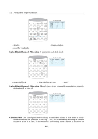
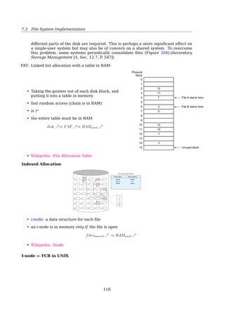
119. 7.4 File System Implementation
partition starts with a boot block, even if it does not contain a bootable operating
system. Besides, it might contain one in the future, so reserving a boot block is a
good idea anyway [19, Sec 4.3.1, File System Layout].
The superblock is read into memory when the computer is booted or the file system is
first touched.
On-Disk Information Structure
Boot control block a MBR copy
UFS: Boot block
NTFS: Partition boot sector
Volume control block Contains volume details
number of blocks size of blocks
free-block count free-block pointers
free FCB count free FCB pointers
UFS: Superblock
NTFS: Master File Table
Directory structure Organizes the files FCB, File control block, contains file details (meta-
data).
UFS: I-node
NTFS: Stored in MFT using a relatiional database structure, with one row per file
Each File-System Has a Superblock
Superblock
Keeps information about the file system
• Type — ext2, ext3, ext4...
• Size
• Status — how it’s mounted, free blocks, free inodes, ...
• Information about other metadata structures
# dumpe2fs /dev/sda1 | grep -i superblock
7.4.2 Implementing Files
Implementing Files
Contiguous Allocation
118

120. 7.4 File System Implementation
dexed.Table 12.3 summarizes some of the characteristics of each method.
With contiguous allocation, a single contiguous set of blocks is allocated to a
file at the time of file creation (Figure 12.7). Thus, this is a preallocation strategy,
using variable-size portions. The file allocation table needs just a single entry for
each file, showing the starting block and the length of the file. Contiguous allocation
is the best from the point of view of the individual sequential file. Multiple blocks
can be read in at a time to improve I/O performance for sequential processing. It is
also easy to retrieve a single block. For example, if a file starts at block b, and the ith
block of the file is wanted, its location on secondary storage is simply b ϩ i Ϫ 1. Con-
tiguous allocation presents some problems. External fragmentation will occur, mak-
ing it difficult to find contiguous blocks of space of sufficient length. From time to
time, it will be necessary to perform a compaction algorithm to free up additional
0 1 2 3 4
5 6 7
File A
File Allocation Table
File B
File C
File E
File D
8 9
10 11 12 13 14
15 16 17 18 19
20 21 22 23 24
25 26 27 28 29
30 31 32 33 34
File Name
File A
File B
File C
File D
File E
2
9
18
30
26
3
5
8
2
3
Start Block Length
Figure 12.7 Contiguous File Allocation
- simple;
- good for read only;
- fragmentation
Linked List (Chained) Allocation A pointer in each disk block
12.6 / SECONDARY STORAGE MANAGEMENT 573
space on the disk (Figure 12.8).Also, with preallocation, it is necessary to declare the
size of the file at the time of creation, with the problems mentioned earlier.
At the opposite extreme from contiguous allocation is chained allocation
(Figure 12.9). Typically, allocation is on an individual block basis. Each block con-
tains a pointer to the next block in the chain. Again, the file allocation table needs
just a single entry for each file, showing the starting block and the length of the file.
Although preallocation is possible, it is more common simply to allocate blocks as
needed.The selection of blocks is now a simple matter: any free block can be added
to a chain. There is no external fragmentation to worry about because only one
Figure 12.9 Chained Allocation
0 1 2 3 4
5 6 7
File A
File Allocation Table
File B
File C
File E File D
8 9
10 11 12 13 14
15 16 17 18 19
20 21 22 23 24
25 26 27 28 29
30 31 32 33 34
File Name
File A
File B
File C
File D
File E
0
3
8
19
16
3
5
8
2
3
Start Block Length
Figure 12.8 Contiguous File Allocation (After Compaction)
0 1 2 3 4
5 6 7
File Allocation Table
File B
8 9
10 11 12 13 14
15 16 17 18 19
20 21 22 23 24
25 26 27 28 29
30 31 32 33 34
File B
File Name Start Block Length
1 5
M12_STAL6329_06_SE_C12.QXD 2/21/08 9:40 PM Page 573
- no waste block; - slow random access; - not 2n
Consolidation One consequence of chaining, as described so far, is that there is no ac-
commodation of the principle of locality. Thus, if it is necessary to bring in several
blocks of a file at a time, as in sequential processing, then a series of accesses to
different parts of the disk are required. This is perhaps a more significant effect on
a single-user system but may also be of concern on a shared system. To overcome
this problem, some systems periodically consolidate files (fig. 304). [18, Sec. 12.7,
Secondary Storage Management, P. 547])
Linked List (Chained) Allocation Though there is no external fragmentation, consoli-
dation is still preferred.
119

121. 7.4 File System Implementation
574 CHAPTER 12 / FILE MANAGEMENT
block at a time is needed.This type of physical organization is best suited to sequen-
tial files that are to be processed sequentially. To select an individual block of a file
requires tracing through the chain to the desired block.
One consequence of chaining, as described so far, is that there is no accommo-
dation of the principle of locality.Thus, if it is necessary to bring in several blocks of
a file at a time, as in sequential processing, then a series of accesses to different parts
of the disk are required. This is perhaps a more significant effect on a single-user
system but may also be of concern on a shared system. To overcome this problem,
some systems periodically consolidate files (Figure 12.10).
Indexed allocation addresses many of the problems of contiguous and chained
allocation. In this case, the file allocation table contains a separate one-level index for
each file; the index has one entry for each portion allocated to the file. Typically, the
file indexes are not physically stored as part of the file allocation table. Rather, the
file index for a file is kept in a separate block, and the entry for the file in the file al-
location table points to that block.Allocation may be on the basis of either fixed-size
blocks (Figure 12.11) or variable-size portions (Figure 12.12). Allocation by blocks
eliminates external fragmentation, whereas allocation by variable-size portions im-
proves locality. In either case, file consolidation may be done from time to time. File
consolidation reduces the size of the index in the case of variable-size portions, but
not in the case of block allocation. Indexed allocation supports both sequential and
direct access to the file and thus is the most popular form of file allocation.
Free Space Management
Just as the space that is allocated to files must be managed, so the space that is not
currently allocated to any file must be managed. To perform any of the file alloca-
tion techniques described previously, it is necessary to know what blocks on the disk
are available. Thus we need a disk allocation table in addition to a file allocation
table.We discuss here a number of techniques that have been implemented.
0 1 2 3 4
5 6 7
File Allocation Table
File B
8 9
10 11 12 13 14
15 16 17 18 19
20 21 22 23 24
25 26 27 28 29
30 31 32 33 34
File B
File Name Start Block Length
0 5
Figure 12.10 Chained Allocation (After Consolidation)
M12_STAL6329_06_SE_C12.QXD 2/21/08 9:40 PM Page 574
FAT: Linked list allocation with a table in RAM
• Taking the pointer out of each disk block, and
putting it into a table in memory
• fast random access (chain is in RAM)
• is 2n
• the entire table must be in RAM
disk ↗⇒ FAT ↗⇒ RAMused ↗
Physical
block
File A starts here
File B starts here
Unused block
0
1
2
3
4
5
6
7
8
9
10
11
12
13
14
15
10
11
7
3
2
12
14
-1
-1
Fig. 6-14. Linked list allocation using a file allocation table in
main memory.
See also [27, File Allocation Table].
Indexed Allocation 12.6 / SECONDARY STORAGE MANAGEMENT 575
Bit Tables This method uses a vector containing one bit for each block on the
disk. Each entry of a 0 corresponds to a free block, and each 1 corresponds to a
block in use. For example, for the disk layout of Figure 12.7, a vector of length 35 is
needed and would have the following value:
00111000011111000011111111111011000
A bit table has the advantage that it is relatively easy to find one or a con-
tiguous group of free blocks. Thus, a bit table works well with any of the file allo-
cation methods outlined. Another advantage is that it is as small as possible.
Figure 12.11 Indexed Allocation with Block Portions
0 1 2 3 4
5 6 7
File Allocation Table
File B
8 9
10 11 12 13 14
15 16 17 18 19
20 21 22 23 24
25 26 27 28 29
30 31 32 33 34
File B
File Name Index Block
24
1
8
3
14
28
0 1 2 3 4
5 6 7
File B
8 9
10 11 12 13 14
15 16 17 18 19
20 21 22 23 24
25 26 27 28 29
Start Block
1
28
14
3
4
1
Length
File Allocation Table
File B
File Name Index Block
24
M12_STAL6329_06_SE_C12.QXD 2/21/08 9:40 PM Page 575
I-node A data structure for each file. An i-node is in memory only if the file is open
filesopened ↗ ⇒ RAMused ↗
See also: [29, Inode]
120

122. 7.4 File System Implementation
I-node — FCB in UNIX
File inode (128B)
Type Mode
User ID Group ID
File size # blocks
# links Flags
Timestamps (×3)
Triple indirect
Double indirect
Single indirect
Direct blocks (×12)
#
#
#
#
2)
Block #s of
more
directory
blocks
File data block
Data
File type Description
0 Unknown
1 Regular file
2 Directory
3 Character device
4 Block device
5 Named pipe
6 Socket
7 Symbolic link
Mode: 9-bit pattern
• in one terminal, to create a file “a”, do:
$ echo hello /tmp/a
• to track its contents and keep it open, do:
$ tail -f a
• in another terminal, delete this file “a”, do:
$ rm -f /tmp/a
• make sure it’s gone, do:
$ ls -l /tmp/a
$ ls -li /proc/`pidof tail`/fd
$ lsof -p `pidof tail` | grep deleted
as you can see, /tmp/a is marked as “deleted”. Now, do:
$ echo another a /tmp/a
$ ls -li /tmp/a
Is this /tmp/a same as the deleted one? (check the inodes)
Inode Quiz
Given:
block size is 1KB
pointer size is 4B
Addressing:
byte offset 9000
byte offset 350,000
121

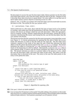
123. 7.4 File System Implementation
+----------------+
0 | 4096 |
+----------------+ ----+----------+ Byte 9000 in a file
1 | 228 | / | 367 | |
+----------------+ / | Data blk | v
2 | 45423 | / +----------+ 8th blk, 808th byte
+----------------+ /
3 | 0 | / --+------+
+----------------+ / / 0| |
4 | 0 | / / +------+
+----------------+ / / : : :
5 | 11111 | / / +------+ Byte 350,000
+----------------+ / -+-----+/ 75| 3333 | in a file
6 | 0 | / / 0| 331 | +------+ |
+----------------+ / / +-----+ : : : v
7 | 101 | / / | | +------+ 816th byte
+----------------+/ / | : | 255| | --+----------+
8 | 367 | / | : | +------+ | 3333 |
+----------------+ / | : | 331 | Data blk |
9 | 0 | / | | Single indirect +----------+
+----------------+ / +-----+
S | 428 (10K+256K) | / 255| |
+----------------+/ +-----+
D | 9156 | 9156 /***********************
+----------------+ Double indirect What about the ZEROs?
T | 824 | ***********************/
+----------------+
Several block entries in the inode are 0, meaning that the logical block entries contain
no data. This happens if no process ever wrote data into the file at any byte offsets cor-
responding to those blocks and hence the block numbers remain at their initial value, 0.
No disk space is wasted for such blocks. Process can cause such a block layout in a file by
using the lseek() and write() system calls [1, Sec. 4.2, Structure of a Regular File].
UNIX In-Core Data Structure
mount table — Info about each mounted FS
directory-structure cache — Dir-info of recently accessed dirs
inode table — An in-core version of the on-disk inode table
file table
• global
• keeps inode of each open file
• keeps track of
– how many processes are associated with each open file
– where the next read and write will start
– access rights
user file descriptor table
• per process
• identifies all open files for a process
Find them in the kernel source
user file descriptor table — struct fdtable in include/linux/fdtable.h
open file table — struct files_struct in include/linux/fdtable.h
inode — struct inode in include/linux/fs.h
inode table — ?
122

124. 7.4 File System Implementation
superblock — struct super_block in include/linux/fs.h
dentry — struct dentry in include/linux/dcache.h
file — struct file in include/linux/fs.h
UNIX In-Core Data Structure
User
File Descriptor
Table
File
Table
Inode
Table
open()/creat()
1. add entry in each table
2. returns a file descriptor — an index into the user file descriptor table
Open file descriptor table A second table, whose address is contained in the files field
of the process descriptor, specifies which files are currently opened by the process. It
is a files_struct structure whose fields are illustrated in Table 12-717
[2, Sec. 12.2.6,
Files Associated with a Process].
The fd field points to an array of pointers to file objects. The size of the array is
stored in the max_fds field. Usually, fd points to the fd_array field of the files_struct
structure, which includes 32 file object pointers. If the process opens more than 32
files, the kernel allocates a new, larger array of file pointers and stores its address in
the fd fields; it also updates the max_fds field.
For every file with an entry in the fd array, the array index is the file descriptor. Usu-
ally, the first element (index 0) of the array is associated with the standard input of
the process, the second with the standard output, and the third with the standard er-
ror (See fig. 12-318
). Unix processes use the file descriptor as the main file identifier.
Notice that, thanks to the dup() , dup2() , and fcntl() system calls, two file descriptors
may refer to the same opened file, that is, two elements of the array could point to
the same file object. Users see this all the time when they use shell constructs such
as 21 to redirect the standard error to the standard output.
open() A call to open() creates a new open file description, an entry in the system-wide
table of open files. This entry records the file offset and the file status flags (modifiable
via the fcntl(2) F_SETFL operation). A file descriptor is a reference to one of these
entries; this reference is unaffected if pathname is subsequently removed or modified
17http://cs2.swfu.edu.cn/pub/resources/Books/Linux/kernel/OREILLY-Understanding_The_Linux_Kernel_3e/
0596005652/understandlk-chp-12-sect-2.html#understandlk-chp-12-table-7
18http://cs2.swfu.edu.cn/pub/resources/Books/Linux/kernel/OREILLY-Understanding_The_Linux_Kernel_3e/
0596005652/understandlk-chp-12-sect-2.html#understandlk-chp-12-fig-3
123

125. 7.4 File System Implementation
to refer to a different file. The new open file description is initially not shared with
any other process, but sharing may arise via fork(2) [man 2 open].
The internal representation of a file is given by an inode, which contains a description
of the disk layout of the file data and other information such as the file owner, access
permissions, and access times. The term inode is a contraction of the term index
node and is commonly used in literature on the UNIX system. Every file has one
inode, but it may have several names, all of which map into the inode. Each name
is called a link. When a process refers to a file by name, the kernel parses the file
name one component at a time, checks that the process has permission to search the
directories in the path, and eventually retrieves the inode for the file. For example,
if a process calls
open(/fs2/mjb/rje/sourcefile,1);
the kernel retrieves the inode for “/fs2/mjb/rje/sourcefile”. When a process creates
a new file, the kernel assigns it an unused inode. Inodes are stored in the file system,
as will be seen shortly, but the kernel reads them into an in-core inode table when
manipulating files.
The kernel contains two other data structures, the file table and the user file descrip-
tor table. The file table is a global kernel structure, but the user file descriptor table
is allocated per process. When a process opens or creats a file, the kernel allocates an
entry from each table, corresponding to the file’s inode. Entries in the three struc-
tures — user file descriptor table, file table, and inode table — maintain the state of
the file and the user’s access to it. The file table keeps track of the byte offset in the
file where the user’s next read or write will start, and the access rights allowed to the
opening process. The user file descriptor table identifies all open files for a process.
Fig. 310 shows the tables and their relationship to each other. The kernel returns
a file descriptor for the open and creat system calls, which is an index into the user
file descriptor table. When executing read and write system calls, the kernel uses the
file descriptor to access the user fie descriptor table, follows pointers to the file table
and inode table entries, and, from the inode, finds the data in the file. Chapters 4
and 5 describe these data structures in great detail. For now, suffice it to say that
use of three tables allows various degrees of sharing access to a file [1, Sec. 2.2.1,
An Overview of the File Subsystem].
The open system call is the first step a process must take to access the data in a file.
The syntax for the open system call is
fd = open(pathname, flags, modes);
where pathname is a file name, flags indicate the type of open (such as for reading
or writing), and modes give the file permissions if the file is being created. The open
system call returns an integer called the user file descriptor. Other file operations,
such as reading, writing, seeking, duplicating the file descriptor, setting file I/O pa-
rameters, determining file status, and closing the file, use the file descriptor that the
open system call returns[1, Sec. 5.1, Open].
The kernel searches the file system for the file name parameter using algorithm namei
(see fig. 1). It checks permissions for opening the file after it finds the in-core inode
and allocates an entry in the file table for the open file. The file table entry contains
a pointer to the inode of the open file and a field that indicates the byte offset in the
file where the kernel expects the next read or write to begin. The kernel initializes
the offset to 0 during the open call, meaning that the initial read or write starts at
the beginning of a file by default. Alternatively, a process can open a file in write-
append mode, in which case the kernel initializes the offset to the size of the file. The
124

126. 7.4 File System Implementation
kernel allocates an entry in a private table in the process u area, called the user file
descriptor table, and notes the index of this entry. The index is the file descriptor
that is returned to the user. The entry in the user file table points to the entry in the
global file table.
algorithm open
inputs: file name
type of open
file permissions (for creation type of open)
output: file descriptor
{
convert file name to inode (algorithm namei);
if (file does not exist or not permitted access)
return (error);
allocate file table entry for inode, initialize count, offset;
allocate user file descriptor entry, set pointer to file table entry;
if (type of open specifies truncate file)
free all file blocks (algorithm free);
unlock (inode); /* locked above in namei */
return (user file descriptor);
}
Figure 1: Algorithm for opening a file
Q1: Can open() return an inode number?
Q2: Can we keep the I/O pointers in the inode? Possibly adding a few pointers in the inode
data structure in a similar fashion of those block pointers (direct/single-indirect/double-
indirect/triple-indirect). Each pointer pointing to an I/O pointer record.
The Tables
Two levels of internal tables in the OS
A per-process table tracks all files that a process has open. Stores
• the current-file-position pointer (not really)
• access rights
• more...
a.k.a file descriptor table
A system-wide table keeps process-independent information, such as
• the location of the file on disk
• access dates
• file size
• file open count — the number of processes opening this file
125

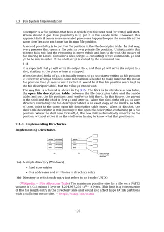
127. 7.4 File System Implementation
Per-process FDT
Process 1
+------------------+ System-wide
| ... | open-file table
+------------------+ +------------------+
| Position pointer | | ... |
| Access rights | +------------------+
| ... | | ... |
+------------------+ +------------------+
| ... | ---------| Location on disk |
+------------------+ | R/W |
| Access dates |
Process 2 | File size |
+------------------+ | Pointer to inode |
| Position pointer | | File-open count |
| Access rights |-----------| ... |
| ... | +------------------+
+------------------+ | ... |
| ... | +------------------+
+------------------+
A process executes the following code:
fd1 = open(/etc/passwd, O_RDONLY);
fd2 = open(local, O_RDWR);
fd3 = open(/etc/passwd, O_WRONLY);
STDIN
STDOUT
STDERR
...
User
File descriptor
table
0
1
2
3
4
5
...
...
count 1
R
...
count 1
RW
...
count 1
W
Global
open file
table
...
...
...
(/etc/passwd)
count 2
...
(local)
count 1
...
Inode table
See also:
• [1, Sec. 5.1, Open].
• File descriptor manipulation19
One more process B:
fd1 = open(/etc/passwd, O_RDONLY);
19http://www.cim.mcgill.ca/~franco/OpSys-304-427/lecture-notes/node27.html#SECTION00063000000000000000
126

128. 7.4 File System Implementation
fd2 = open(private, O_RDONLY);
STDIN
STDOUT
STDERR
...
Proc B
User
File descriptor
table
0
1
2
3
4
5
...
...
count 1
R
...
count 1
RW
...
count 1
R
...
count 1
W
...
count 1
R
Global
open file
table
...
...
(/etc/passwd)
count 3
...
...
(local)
count 1
...
...
(private)
count 1
...
...
Inode table
STDIN
STDOUT
STDERR
...
Proc B
0
1
2
3
4
...
Why File Table?
To allow a parent and child to share a file position, but to provide unrelated processes
with their own values.
Mode
i-node
Link count
Uid
Gid
File size
Times
Addresses of
first 10
disk blocks
Single indirect
Double indirect
Triple indirect
Parent’s
file
descriptor
table
Child’s
file
descriptor
table
Unrelated
process
file
descriptor
table
Open file
description
File position
R/W
Pointer to i-node
File position
R/W
Pointer to i-node
Pointers to
disk blocks
Triple
indirect
block Double
indirect
block
Single
indirect
block
‘
Fig. 10-33. The relation between the file descriptor table, the open
file description table, and the i-node table.
Why File Table?
Where To Put File Position Info?
Inode table? No. Multiple processes can open the same file. Each one has its own file
position.
User file descriptor table? No. Trouble in file sharing.
127

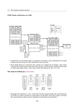
129. 7.4 File System Implementation
Example
#!/bin/bash
echo hello
echo world
Where should the “world” be?
$ ./hello.sh A
Why file table?
File system implementation With file sharing, it is necessary to allow related pro-
cesses to share a common I/O pointer and yet have separate I/O pointers for
independent processes that access the same file. With these two conditions,
the I/O pointer cannot reside in the i-node table nor can it reside in the list of
open files for the process. A new table (the open file table) was invented for the
sole purpose of holding the I/O pointer. Processes that share the same open file
(the result of forks) share a common open file table entry. A separate open of
the same file will only share the i-node table entry, but will have distinct open
file table entries [20, Sec. 4.1].
Open The user file descriptor table entry could conceivably contain the file offset
for the position of the next I/O operation and point directly to the in-core inode
entry for the file, eliminating the need for a separate kernel file table. The exam-
ples above show a one-to-one relationship between user file descriptor entries
and kernel file table entries. Thompson notes, however, that he implemented
the file table as a separate structure to allow sharing of the offset pointer be-
tween several user file descriptors (see [20, Thompson 78, p. 1943]). The dup
and fork system calls, explained in [1, Sec. 5.13] and [1, Sec. 7.1], manipulate
the data structures to allow such sharing [1, Sec. 5.1].
The Linux File System ... The idea is to start with this file descriptor and end up
with the corresponding i-node. Let us consider one possible design: just put a
pointer to the i-node in the file descriptor table. Although simple, unfortunately
this method does not work. The problem is as follows. Associated with every
file descriptor is a file position that tells at which byte the next read (or write)
will start. Where should it go? One possibility is to put it in the i-node table.
However, this approach fails if two or more unrelated processes happen to open
the same file at the same time because each one has its own file position [19,
Sec. 10.6].
A second possibility is to put the file position in the file descriptor table. In that
way, every process that opens a file gets its own private file position. Unfor-
tunately this scheme fails too, but the reasoning is more subtle and has to do
with the nature of file sharing in Linux. Consider a shell script, s, consisting of
two commands, p1 and p2, to be run in order. If the shell script is called by the
command line
S X
it is expected that p1 will write its output to x, and then p2 will write its output
to x also, starting at the place where p1 stopped.
When the shell forks off p1, x is initially empty, so p1 just starts writing at file
position 0. However, when p1 finishes, some mechanism is needed to make
sure that the initial file position that p2 sees is not 0 (which it would be if the
file position were kept in the file descriptor table), but the value p1 ended with.
The way this is achieved is shown in Fig 315. The trick is to introduce a new
table, the open file description table, between the file descriptor table and the
128

130. 7.4 File System Implementation
i-node table, and put the file position (and read/write bit) there. In this figure,
the parent is the shell and the child is first p1 and later p2. When the shell
forks off p1, its user structure (including the file descriptor table) is an exact
copy of the shell’s, so both of them point to the same open file description table
entry. When p1 finishes, the shell’s file descriptor is still pointing to the open
file description containing p1’s file position. When the shell now forks off p2,
the new child automatically inherits the file position, without either it or the
shell even having to know what that position is.
7.4.3 Implementing Directories
Implementing Directories
(a)
games
mail
news
work
attributes
attributes
attributes
attributes
Data structure
containing the
attributes
(b)
games
mail
news
work
Fig. 6-16. (a) A simple directory containing fixed-size entries with
the disk addresses and attributes in the directory entry. (b) A direc-
tory in which each entry just refers to an i-node.
(a) A simple directory (Windows)
– fixed size entries
– disk addresses and attributes in directory entry
(b) Directory in which each entry just refers to an i-node (UNIX)
The maximum possible size for a file on a FAT32 volume is 4 GiB minus 1 byte or
4,294,967,295 (232
−1) bytes. This limit is a consequence of the file length entry in the
directory table and would also affect huge FAT16 partitions with a sufficient sector size
[27, File Allocation Table].
How Long A File Name Can Be?
File 1 entry length
File 1 attributes
Pointer to file 1's name
File 1 attributes
Pointer to file 2's name
File 2 attributes
Pointer to file 3's name
File 2 entry length
File 2 attributes
File 3 entry length
File 3 attributes
p
e
b
e
r
c
u
t
o
t
d
j
-
g
p
e
b
e
r
c
u
t
o
t
d
j
-
g
p
e r s o
n n e l
f o o
p
o
l
e
n
r
n
f o o
s
e
Entry
for one
file
Heap
Entry
for one
file
(a) (b)
File 3 attributes
129

131. 7.4 File System Implementation
How long file name is implemented?
1. The simplest approach is to set a limit on file name length, typically 255 char-
acters, and then use one of the designs of fig. 317 with 255 characters reserved
for each file name. This approach is simple, but wastes a great deal of directory
space, since few files have such long names. For efficiency reasons, a different
structure is desirable.
2. One alternative is to give up the idea that all directory entries are the same size.
With this method, each directory entry contains a fixed portion, typically start-
ing with the length of the entry, and then followed by data with a fixed format,
usually including the owner, creation time, protection information, and other
attributes. This fixed-length header is followed by the actual file name, how-
ever long it may be, as shown in fig. 318(a) in big-endian format (e.g., SPARC).
In this example we have three files, project-budget, personnel, and foo. Each
file name is terminated by a special character (usually 0), which is represented
in the figure by a box with a cross in it. To allow each directory entry to begin
on a word boundary, each file name is filled out to an integral number of words,
shown by shaded boxes in the figure.
A disadvantage of this method is that when a file is removed, a variable-sized
gap is introduced into the directory into which the next file to be entered may
not fit. This problem is the same one we saw with contiguous disk files, only now
compacting the directory is feasible because it is entirely in memory. Another
problem is that a single directory entry may span multiple pages, so a page
fault may occur while reading a file name.
3. Another way to handle variable-length names is to make the directory entries
themselves all fixed length and keep the file names together in a heap at the end
of the directory, as shown in fig. 318(b). This method has the advantage that
when an entry is removed, the next file entered will always fit there. Of course,
the heap must be managed and page faults can still occur while processing file
names. One minor win here is that there is no longer any real need for file
names to begin at word boundaries, so no filler characters are needed after file
names in fig. 318(b) as they are in fig. 318(a).
4. Ext2’s approach is a bit different. See Sec. 7.5.5.
See also: [19, Sec. 4.3.3, Implementating Directories]
UNIX Treats a Directory as a File
130

132. 7.4 File System Implementation
Directory inode (128B)
Type Mode
User ID Group ID
File size # blocks
# links Flags
Timestamps (×3)
Triple indirect
Double indirect
Single indirect
Direct blocks (×12)
.
..
passwd
fstab
… …
Directory block
File inode (128B)
Type Mode
User ID Group ID
File size # blocks
# links Flags
Timestamps (×3)
Triple indirect
Double indirect
Single indirect
Direct blocks (×12)
Indirect block
inode #
inode #
inode #
inode #
Direct blocks (×512)
Block #s of
more
directory
blocks
Block # of
block with
512 single
indirect
entries
Block # of
block with
512 double
indirect
entries
File data block
Data
Example
. 2
.. 2
bin 11116545
boot 2
cdrom 12
dev 3
.
.
.
.
.
.
• A directory is a file whose data is a sequence of entries, each consisting of an inode
number and the name of a file contained in the directory.
• Each (disk) block in a directory file consists of a linked list of entries; each entry
contains the length of the entry, the name of a file, and the inode number of the inode
to which that entry refers[17, Sec. 15.7.2, The Linux ext2fs File System].
The steps in looking up /usr/ast/mbox
Root directory
I-node 6
is for /usr
Block 132
is /usr
directory
I-node 26
is for
/usr/ast
Block 406
is /usr/ast
directory
Looking up
usr yields
i-node 6
I-node 6
says that
/usr is in
block 132
/usr/ast
is i-node
26
/usr/ast/mbox
is i-node
60
I-node 26
says that
/usr/ast is in
block 406
1
1
4
7
14
9
6
8
.
..
bin
dev
lib
etc
usr
tmp
6
1
19
30
51
26
45
dick
erik
jim
ast
bal
26
6
64
92
60
81
17
grants
books
mbox
minix
src
Mode
size
times
132
Mode
size
times
406
• First the file system locates the root directory. In UNIX its i-node is located at a
fixed place on the disk. From this i-node, it locates the root directory, which can be
anywhere on the disk, but say block 1[19, Sec. 4.5, Example File Systems].
131

133. 7.4 File System Implementation
Then it reads the root directory and looks up the first component of the path, usr,
in the root directory to find the i-node number of the file /usr. Locating an i-node
from its number is straightforward, since each one has a fixed location on the disk.
From this i-node, the system locates the directory for /usr and looks up the next
component, ast, in it. When it has found the entry for ast, it has the i-node for the
directory /usr/ast. From this i-node it can find the directory itself and look up mbox.
The i-node for this file is then read into memory and kept there until the file is closed.
The lookup process is illustrated in fig. 320.
Relative path names are looked up the same way as absolute ones, only starting from
the working directory instead of starting from the root directory. Every directory has
entries for . and .. which are put there when the directory is created. The entry .
has the i-node number for the current directory, and the entry for .. has the i-node
number for the parent directory. Thus, a procedure looking up ../dick/prog.c simply
looks up .. in the working directory, finds the i-node number for the parent directory,
and searches that directory for dick. No special mechanism is needed to handle these
names. As far as the directory system is concerned, they are just ordinary ASCII
strings, just the same as any other names. The only bit of trickery here is that .. in
the root directory points to itself.
7.4.4 Shared Files
File Sharing
Multiple Users
User IDs identify users, allowing permissions and protections to be per-user
Group IDs allow users to be in groups, permitting group access rights
Example: 9-bit pattern
rwxr-x--- means:
user group other
rwx r-x ---
111 1-1 000
7 5 0
File Sharing
Remote File Systems
Networking — allows file system access between systems
– Manually via programs like FTP
– Automatically, seamlessly using distributed file systems
– Semi automatically, via the world wide web
C/S model — allows clients to mount remote file systems from servers
– NFS — standard UNIX client-server file sharing protocol
– CIFS — standard Windows protocol
– Standard system calls are translated into remote calls
Distributed Information Systems (distributed naming services)
– such as LDAP, DNS, NIS, Active Directory implement unified access to informa-
tion needed for remote computing
132

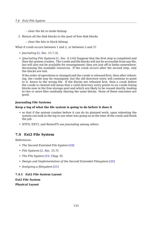
134. 7.4 File System Implementation
File Sharing
Protection
• File owner/creator should be able to control:
– what can be done
– by whom
• Types of access
– Read
– Write
– Execute
– Append
– Delete
– List
Shared Files
Hard Links vs. Soft Links
Root directory
B
B B C
C C
CA
B C
B
? C C C
A
Shared file
Fig. 6-18. File system containing a shared file.
See also: [24, Directed acyclic graph].
Hard Links
Hard links

135. the same inode
Drawback
133

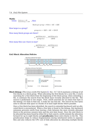
136. 7.4 File System Implementation
C's directory B's directory B's directoryC's directory
Owner = C
Count = 1
Owner = C
Count = 2
Owner = C
Count = 1
(a) (b) (c)
• Both hard and soft links have drawbacks[19, Sec. 4.3.4, Shared Files].
• echo 0 /proc/sys/fs/protected_hardlinks
• Why hard links not allowed to directories in UNIX/Linux20
?
... if you were allowed to do this for directories, two different directories in different
points in the filesystem could point to the same thing. In fact, a subdir could point
back to its grandparent, creating a loop.
Why is this loop a concern? Because when you are traversing, there is no way to
detect you are looping (without keeping track of inode numbers as you traverse).
Imagine you are writing the du command, which needs to recurse through subdirs to
find out about disk usage. How would du know when it hit a loop? It is error prone
and a lot of bookkeeping that du would have to do, just to pull off this simple task.
• The Ultimate Linux Soft and Hard Link Guide (10 Ln Command Examples)21
Symbolic Links
A symbolic link has its own inode

137. a directory entry.
7.4.5 Disk Space Management
Disk Space Management
Statistics
20http://unix.stackexchange.com/questions/22394/why-hard-links-not-allowed-to-directories-in-unix-linux
21http://www.thegeekstuff.com/2010/10/linux-ln-command-examples/
134

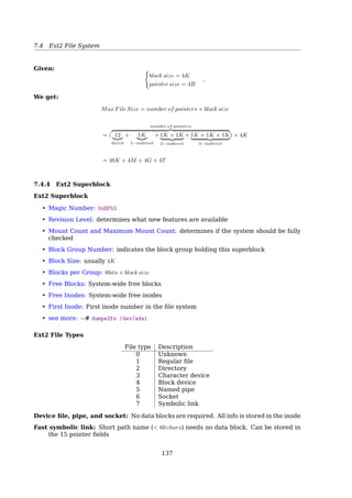
138. 7.4 File System Implementation
See also: [19, Sec. 4.4.1, Disk Space Management].
• Block size is chosen while creating the FS
• Disk I/O performance is conflict with space utilization
– smaller block size ⇒ better space utilization
– larger block size ⇒ better disk I/O performance
$ dumpe2fs /dev/sda1 | grep Block size
Keeping Track of Free Blocks
1. Linked List10.5 Free-Space Management 443
0 1 2 3
4 5 7
8 9 10 11
12 13 14
16 17 18 19
20 21 22 23
24 25 26 27
28 29 30 31
15
6
free-space list head
Figure 10.10 Linked free-space list on disk.
of free blocks can now be found quickly, unlike the situation
d linked-list approach is used.
ng
h takes advantage of the fact that, generally, several contigu-
allocated or freed simultaneously, particularly when space is
contiguous-allocation algorithm or through clustering. Thus,
ng a list of n free disk addresses, we can keep the address of
and the number (n) of free contiguous blocks that follow the
ntry in the free-space list then consists of a disk address and
h each entry requires more space than would a simple disk
ll list is shorter, as long as the count is generally greater than
method of tracking free space is similar to the extent method
ks. These entries can be stored in a B-tree, rather than a linked
okup, insertion, and deletion.
2. Bit map (n blocks)
0 1 2 3 4 5 6 7 8 .. n-1
+-+-+-+-+-+-+-+-+-+-//-+-+
|0|0|1|0|1|1|1|0|1| .. |0|
+-+-+-+-+-+-+-+-+-+-//-+-+
bit[i] =
{
0 ⇒ block[i] is free
1 ⇒ block[i] is occupied
Journaling File Systems
Operations required to remove a file in UNIX:
1. Remove the file from its directory
- set inode number to 0
2. Release the i-node to the pool of free i-nodes
135

139. 7.5 Ext2 File System
- clear the bit in inode bitmap
3. Return all the disk blocks to the pool of free disk blocks
- clear the bits in block bitmap
What if crash occurs between 1 and 2, or between 2 and 3?
Suppose that the first step is completed and then the system crashes. The i-node and file
blocks will not be accessible from any file, but will also not be available for reassignment;
they are just off in limbo somewhere, decreasing the available resources. If the crash
occurs after the second step, only the blocks are lost.
If the order of operations is changed and the i-node is released first, then after reboot-
ing, the i-node may be reassigned, but the old directory entry will continue to point to it,
hence to the wrong file. If the blocks are released first, then a crash before the i-node
is cleared will mean that a valid directory entry points to an i-node listing blocks now in
the free storage pool and which are likely to be reused shortly, leading to two or more
files randomly sharing the same blocks. None of these outcomes are good[19, Sec. 4.3.6,
Journaling File Systems].
See also: [17, Sec. 15.7.3, Journaling].
Journaling File Systems
Keep a log of what the file system is going to do before it does it
• so that if the system crashes before it can do its planned work, upon rebooting the
system can look in the log to see what was going on at the time of the crash and finish
the job.
• NTFS, EXT3, and ReiserFS use journaling among others
7.5 Ext2 File System
References:
• [15, The Second Extented File System]
• [17, Sec. 15.7, File Systems]
• [16, Chap. 9, The File System]
• [4, Design and Implementation of the Second Extended Filesystem]
• [13, Analyzing a filesystem]
7.5.1 Ext2 File System Layout
Ext2 File System
Physical Layout
+------------+---------------+---------------+--//--+---------------+
| Boot Block | Block Group 0 | Block Group 1 | | Block Group n |
+------------+---------------+---------------+--//--+---------------+
__________________________/ _____________
/
+-------+-------------+------------+--------+-------+--------+
| Super | Group | Data Block | inode | inode | Data |
| Block | Descriptors | Bitmap | Bitmap | Table | Blocks |
+-------+-------------+------------+--------+-------+--------+
1 blk n blks 1 blk 1 blk n blks n blks
136

140. 7.5 Ext2 File System
See also: [17, Sec. 15.7.2, The Linux ext2fs File System].
7.5.2 Ext2 Block groups
Ext2 Block groups
The partition is divided into Block Groups
• Block groups are same size — easy locating
• Kernel tries to keep a file’s data blocks in the same block group — reduce fragmen-
tation
• Backup critical info in each block group
• The Ext2 inodes for each block group are kept in the inode table
• The inode-bitmap keeps track of allocated and unallocated inodes
When allocating a file, ext2fs must first select the block group for that file[17,
Sec. 15.7.2, The Linux ext2fs File System, P. 625].
• For data blocks, it attempts to allocate the file to the block group to which
the file’s inode has been allocated.
• For inode allocations, it selects the block group in which the file’s parent
directory resides, for nondirectory files.
• Directory files are not kept together but rather are dispersed throughout
the available block groups.
These policies are designed not only to keep related information within the same
block group but also to spread out the disk load among the disk’s block groups
to reduce the fragmentation of any one area of the disk.
Group descriptor
• Each block group has a group descriptor
• All the group descriptors together make the group descriptor table
• The table is stored along with the superblock
• Block Bitmap: tracks free blocks
• Inode Bitmap: tracks free inodes
• Inode Table: all inodes in this block group
•
Free blocks count
Free Inodes count
Used dir count
}
counters
See more: # dumpe2fs /dev/sda1
137

141. 7.5 Ext2 File System
Maths
Given
block size = 4K
block bitmap = 1 blk
, then
blocks per group = 8 bits × 4K = 32K
How large is a group?
group size = 32K × 4K = 128 M
How many block groups are there?
≈
partition size
group size
=
partition size
128M
How many files can I have in max?
≈
partition size
block size
=
partition size
4K
Ext2 Block Allocation Policies626 Chapter 15 The Linux System
allocating scattered free blocks
allocating continuous free blocks
block in use bit boundary
block selected
by allocator
free block byte boundarybitmap search
Figure 15.9 ext2fs block-allocation policies.
these extra blocks to the file. This preallocation helps to reduce fragmentation
during interleaved writes to separate files and also reduces the CPU cost of
disk allocation by allocating multiple blocks simultaneously. The preallocated
blocks are returned to the free-space bitmap when the file is closed.
Figure 15.9 illustrates the allocation policies. Each row represents a
sequence of set and unset bits in an allocation bitmap, indicating used and
free blocks on disk. In the first case, if we can find any free blocks sufficiently
near the start of the search, then we allocate them no matter how fragmented
they may be. The fragmentation is partially compensated for by the fact that
the blocks are close together and can probably all be read without any disk
seeks, and allocating them all to one file is better in the long run than allocating
isolated blocks to separate files once large free areas become scarce on disk. In
the second case, we have not immediately found a free block close by, so we
search forward for an entire free byte in the bitmap. If we allocated that byte
as a whole, we would end up creating a fragmented area of free space between
it and the allocation preceding it, so before allocating we back up to make this
allocation flush with the allocation preceding it, and then we allocate forward
to satisfy the default allocation of eight blocks.
15.7.3 Journaling
One popular feature in a file system is journaling, whereby modifications
to the file system are sequentially written to a journal. A set of operations
Block bitmap It maintains a bitmap of all free blocks in a block group. When allocating
the first blocks for a new file, it starts searching for a free block from the beginning of
the block group; when extending a file, it continues the search from the block most
recently allocated to the file. The search is performed in two stages. First, ext2fs
searches for an entire free byte in the bitmap; if it fails to find one, it looks for any
free bit. The search for free bytes aims to allocate disk space in chunks of at least
eight blocks where possible[17, Sec. 15.7.2, The Linux ext2fs File System].
Once a free block has been identified, the search is extended backward until an allo-
cated block is encountered. When a free byte is found in the bitmap, this backward
extension prevents ext2fs from leaving a hole between the most recently allocated
block in the previous nonzero byte and the zero byte found. Once the next block to
be allocated has been found by either bit or byte search, ext2fs extends the allocation
forward for up to eight blocks and preallocates these extra blocks to the file. This
preallocation helps to reduce fragmentation during interleaved writes to separate
138

142. 7.5 Ext2 File System
files and also reduces the CPU cost of disk allocation by allocating multiple blocks
simultaneously. The preallocated blocks are returned to the free-space bitmap when
the file is closed.
Fig. 337 illustrates the allocation policies. Each row represents a sequence of set
and unset bits in an allocation bitmap, indicating used and free blocks on disk. In
the first case, if we can find any free blocks sufficiently near the start of the search,
then we allocate them no matter how fragmented they may be. The fragmentation
is partially compensated for by the fact that the blocks are close together and can
probably all be read without any disk seeks, and allocating them all to one file is
better in the long run than allocating isolated blocks to separate files once large free
areas become scarce on disk. In the second case, we have not immediately found a
free block close by, so we search forward for an entire free byte in the bitmap. If
we allocated that byte as a whole, we would end up creating a fragmented area of
free space between it and the allocation preceding it, so before allocating we back
up to make this allocation flush with the allocation preceding it, and then we allocate
forward to satisfy the default allocation of eight blocks.
7.5.3 Ext2 Inode
Ext2 inode
Ext2 inode
Mode: holds two pieces of information
1. Is it a {file|dir|sym-link|blk-dev|char-dev|FIFO}?
2. Permissions
Owner info: Owners’ ID of this file or directory
Size: The size of the file in bytes
Timestamps: Accessed, created, last modified time
Datablocks: 15 pointers to data blocks (12 + S + D + T)
Max File Size
139

143. 7.5 Ext2 File System
Given: {
block size = 4K
pointer size = 4B
,
We get:
Max File Size = number of pointers × block size
= (
number of pointers
12
direct
+ 1K
1−indirect
+ 1K × 1K
2−indirect
+ 1K × 1K × 1K
3−indirect
) × 4K
= 48K + 4M + 4G + 4T
7.5.4 Ext2 Superblock
Ext2 Superblock
Magic Number: 0xEF53
Revision Level: determines what new features are available
Mount Count and Maximum Mount Count: determines if the system should be fully
checked
Block Group Number: indicates the block group holding this superblock
Block Size: usually 4K
Blocks per Group: 8bits × block size
Free Blocks: System-wide free blocks
Free Inodes: System-wide free inodes
First Inode: First inode number in the file system
See more: ∼# dumpe2fs /dev/sda1
Ext2 File Types
File type Description
0 Unknown
1 Regular file
2 Directory
3 Character device
4 Block device
5 Named pipe
6 Socket
7 Symbolic link
Device file, pipe, and socket: No data blocks are required. All info is stored in the inode
Fast symbolic link: Short path name ( 60 chars) needs no data block. Can be stored in
the 15 pointer fields
140

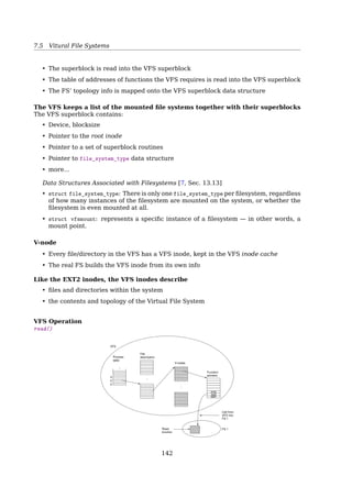
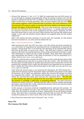
144. 7.6 Vitural File Systems
7.5.5 Ext2 Directory
Ext2 Directories
0 11|12 23|24 39|40
+----+--+-+-+----+----+--+-+-+----+----+--+-+-+----+----+--//--+
| 21 |12|1|2|. | 22 |12|2|2|.. | 53 |16|5|2|hell|o | |
+----+--+-+-+----+----+--+-+-+----+----+--+-+-+----+----+--//--+
,-------- inode number
| ,--- record length
| | ,--- name length
| | | ,--- file type
| | | | ,---- name
+----+--+-+-+----+
0 | 21 |12|1|2|. |
+----+--+-+-+----+
12| 22 |12|2|2|.. |
+----+--+-+-+----+----+
24| 53 |16|5|2|hell|o |
+----+--+-+-+----+----+
40| 67 |28|3|2|usr |
+----+--+-+-+----+----+
52| 0 |16|7|1|oldf|ile |
+----+--+-+-+----+----+
68| 34 |12|4|2|sbin|
+----+--+-+-+----+
• Directories are special files
• “.” and “..” first
• Padding to 4 ×
• inode number is 0 — deleted file
Directory files are stored on disk just like normal files, although their contents are
interpreted differently. Each block in a directory file consists of a linked list of entries;
each entry contains the length of the entry, the name of a file, and the inode number of
the inode to which that entry refers[17, Sec. 15.7.2, The Linux ext2fs File System].
7.6 Vitural File Systems
Many different FS are in use
Windows
uses drive letter (C:, D:, ...) to identify each FS
UNIX
integrates multiple FS into a single structure
– From user’s view, there is only one FS hierarchy
$ man fs
Windows handles these disparate file systems by identifying each one with a different
drive letter, as in C:, D:, etc. When a process opens a file, the drive letter is explicitly
or implicitly present so Windows knows which file system to pass the request to. There
is no attempt to integrate heterogeneous file systems into a unified whole[19, Sec. 4.3.7,
Virtual File Systems].
$ cp /floppy/TEST /tmp/test
141

145. 7.6 Vitural File Systems
cp
VFS
ext2 MS-DOS
/tmp/test /floppy/TEST
1 inf = open(/floppy/TEST, O_RDONLY, 0);
2 outf = open(/tmp/test,
3 O_WRONLY|O_CREAT|O_TRUNC, 0600);
4 do {
5 i = read(inf, buf, 4096);
6 write(outf, buf, i);
7 } while (i);
8 close(outf);
9 close(inf);
Where /floppy is the mount point of an MS-DOS diskette and /tmp is a normal Second
Extended Filesystem (Ext2) directory. The VFS is an abstraction layer between the ap-
plication program and the filesystem implementations. Therefore, the cp program is not
required to know the filesystem types of /floppy/TEST and /tmp/test. Instead, cp inter-
acts with the VFS by means of generic system calls known to anyone who has done Unix
programming[2, Sec. 12.1].
ret = write(fd, buf, len);
263Unix Filesystems
sys_write() system call that determines the actual file writing method for the filesystem
on which fd resides.The generic write system call then invokes this method, which is part
of the filesystem implementation, to write the data to the media (or whatever this filesys-
tem does on write). Figure 13.2 shows the flow from user-space’s write() call through
the data arriving on the physical media. On one side of the system call is the genericVFS
interface, providing the frontend to user-space; on the other side of the system call is the
filesystem-specific backend, dealing with the implementation details.The rest of this chap-
ter looks at how theVFS achieves this abstraction and provides its interfaces.
Unix Filesystems
Historically, Unix has provided four basic filesystem-related abstractions: files, directory
entries, inodes, and mount points.
A filesystem is a hierarchical storage of data adhering to a specific structure. Filesystems
contain files, directories, and associated control information.Typical operations performed
on filesystems are creation, deletion, and mounting. In Unix, filesystems are mounted at a
specific mount point in a global hierarchy known as a namespace.1
This enables all
mounted filesystems to appear as entries in a single tree. Contrast this single, unified tree
with the behavior of DOS and Windows, which break the file namespace up into drive
letters, such as C:.This breaks the namespace up among device and partition boundaries,
“leaking” hardware details into the filesystem abstraction.As this delineation may be arbi-
trary and even confusing to the user, it is inferior to Linux’s unified namespace.
A file is an ordered string of bytes.The first byte marks the beginning of the file, and
the last byte marks the end of the file. Each file is assigned a human-readable name for
identification by both the system and the user.Typical file operations are read, write,
1
Recently, Linux has made this hierarchy per-process, to give a unique namespace to each process.
Because each process inherits its parent’s namespace (unless you specify otherwise), there is seem-
ingly one global namespace.
user-space VFS filesystem physical media
write( ) sys_write( )
filesystem’s
write method
Figure 13.2 The flow of data from user-space issuing a write() call, through the
VFS’s generic system call, into the filesystem’s specific write method, and finally
arriving at the physical media.
This system call writes the len bytes pointed to by buf into the current position in the
file represented by the file descriptor fd. This system call is first handled by a generic
sys_write() system call that determines the actual file writing method for the filesystem
on which fd resides. The generic write system call then invokes this method, which is
part of the filesystem implementation, to write the data to the media (or whatever this
filesystem does on write). Fig. 346 shows the flow from user-space’s write() call through
the data arriving on the physical media. On one side of the system call is the generic
VFS interface, providing the frontend to user-space; on the other side of the system call
is the filesystem-specific backend, dealing with the implementation details[11, Sec. 13.2,
P. 262].
Virtural File Systems
Put common parts of all FS in a separate layer
• It’s a layer in the kernel
• It’s a common interface to several kinds of file systems
• It calls the underlying concrete FS to actual manage the data
142

146. 7.6 Vitural File Systems
User
process
FS 1 FS 2 FS 3
Buffer cache
Virtual file system
File
system
VFS interface
POSIX
• To the VFS layer and the rest of the kernel, however, each filesystem looks the same.
They all support notions such as files and directories, and they all support operations
such as creating and deleting files. ... In fact, nothing in the kernel needs to under-
stand the underlying details of the filesystems, except the filesystems themselves[11,
Sec. 13.2, Filesystem Abstraction Layer].
• The key idea is to abstract out that part of the file system that is common to all file
systems and put that code in a separate layer that calls the underlying concrete file
systems to actual manage the data[19, Sec. 4.3.7, Virtual File Systems]. The overall
structure is illustrated in Fig 347.
All system calls relating to files are directed to the virtual file system for initial pro-
cessing. These calls, coming from user processes, are the standard POSIX calls, such
as open, read, write, lseek, and so on. Thus the VFS has an “upper” interface to user
processes and it is the well-known POSIX interface.
The VFS also has a “lower” interface to the concrete file systems, which is labeled
VFS interface in fig. 347 . This interface consists of several dozen function calls that
the VFS can make to each file system to get work done. Thus to create a new file
system that works with the VFS, the designers of the new file system must make sure
that it supplies the function calls the VFS requires.
Virtual File System
• Manages kernel level file abstractions in one format for all file systems
• Receives system call requests from user level (e.g. write, open, stat, link)
• Interacts with a specific file system based on mount point traversal
• Receives requests from other parts of the kernel, mostly from memory management
Real File Systems
• managing file directory data
• managing meta-data: timestamps, owners, protection, etc.
• disk data, NFS data...
translate
←−−−−−→ VFS data
Historically, Unix has provided four basic filesystem-related abstractions: files, direc-
tory entries, inodes, and mount points[11, Sec. 13.3, Unix Filesystems].
A filesystem is a hierarchical storage of data adhering to a specific structure. Filesys-
tems contain files, directories, and associated control information.Typical operations per-
formed on filesystems are creation, deletion, and mounting. In Unix, filesystems are
143

147. 7.6 Vitural File Systems
mounted at a specific mount point in a global hierarchy known as a namespace. This
enables all mounted filesystems to appear as entries in a single tree. Contrast this single,
unified tree with the behavior of DOS and Windows, which break the file namespace up
into drive letters, such as C:. This breaks the namespace up among device and partition
boundaries, “leaking” hardware details into the filesystem abstraction. As this delineation
may be arbitrary and even confusing to the user, it is inferior to Linux’s unified namespace.
... Traditionally, Unix filesystems implement these notions as part of their physical on-
disk layout. For example, file information is stored as an inode in a separate block on the
disk; directories are files; control information is stored centrally in a superblock, and so
on. The Unix file concepts are physically mapped on to the storage medium. The Linux
VFS is designed to work with filesystems that understand and implement such concepts.
Non-Unix filesystems, such as FAT or NTFS, still work in Linux, but their filesystem code
must provide the appearance of these concepts. For example, even if a filesystem does not
support distinct inodes, it must assemble the inode data structure in memory as if it did.
Or if a filesystem treats directories as a special object, to the VFS they must represent
directories as mere files. Often, this involves some special processing done on-the-fly by
the non-Unix filesystems to cope with the Unix paradigm and the requirements of the VFS.
Such filesystems still work, however, and the overhead is not unreasonable.
File System Mounting
/
a b a
c
p q r q q r
d
/
c d
b
Diskette
/
Hard diskHard disk
x y z
x y z
Fig. 10-26. (a) Separate file systems. (b) After mounting.A FS must be mounted before it can be used
Mount — The file system is registered with the VFS
• The superblock is read into the VFS superblock
• The table of addresses of functions the VFS requires is read into the VFS superblock
• The FS’ topology info is mapped onto the VFS superblock data structure
The VFS keeps a list of the mounted file systems together with their superblocks
The VFS superblock contains:
• Device, blocksize
• Pointer to the root inode
• Pointer to a set of superblock routines
• Pointer to file_system_type data structure
• more...
144

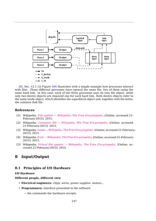
148. 7.6 Vitural File Systems
See also: [11, Sec. 13.13, Data Structures Associated with Filesystems]
• struct file_system_type: There is only one file_system_type per filesystem, regardless
of how many instances of the filesystem are mounted on the system, or whether the
filesystem is even mounted at all.
• struct vfsmount: represents a specific instance of a filesystem — in other words, a
mount point.
V-node
• Every file/directory in the VFS has a VFS inode, kept in the VFS inode cache
• The real FS builds the VFS inode from its own info
Like the EXT2 inodes, the VFS inodes describe
• files and directories within the system
• the contents and topology of the Virtual File System
VFS Operation
read()
...
Process
table
0
File
descriptors
...
V-nodes
open
read
write
Function
pointers
...2
4
VFS
Read
function
FS 1
Call from
VFS into
FS 1
To understand how the VFS works, let us run through an example chronologically.
When the system is booted, the root file system is registered with the VFS. In addition,
when other file systems are mounted, either at boot time or during operation, they, too
must register with the VFS. When a file system registers, what it basically does is provide
a list of the addresses of the functions the VFS requires, either as one long call vector
(table) or as several of them, one per VFS object, as the VFS demands. Thus once a file
system has registered with the VFS, the VFS knows how to, say, read a block from it —
it simply calls the fourth (or whatever) function in the vector supplied by the file system.
Similarly, the VFS then also knows how to carry out every other function the concrete file
system must supply: it just calls the function whose address was supplied when the file
system registered[19, Sec. 4.3.7, Virtual File Systems, P. 288].
After a file system has been mounted, it can be used. For example, if a file system has
been mounted on /usr and a process makes the call
145

149. 7.6 Vitural File Systems
open(/usr/include/unistd.h, O_RDONLY);
while parsing the path, the VFS sees that a new file system has been mounted on /usr
and locates its superblock by searching the list of superblocks of mounted file systems.
Having done this, it can find the root directory of the mounted file system and look up
the path include/unistd.h there. The VFS then creates a v-node and makes a call to the
concrete file system to return all the information in the file’s i-node. This information
is copied into the v-node (in RAM), along with other information, most importantly the
pointer to the table of functions to call for operations on v-nodes, such as read, write,
close, and so on.
After the v-node has been created, the VFS makes an entry in the file descriptor table
for the calling process and sets it to point to the new v-node. (For the purists, the file
descriptor actually points to another data structure that contains the current file position
and a pointer to the v-node, but this detail is not important for our purposes here.) Finally,
the VFS returns the file descriptor to the caller so it can use it to read, write, and close
the file.
Later when the process does a read using the file descriptor, the VFS locates the v-node
from the process and file descriptor tables and follows the pointer to the table of functions,
all of which are addresses within the concrete file system on which the requested file
resides. The function that handles read is now called and code within the concrete file
system goes and gets the requested block. The VFS has no idea whether the data are
coming from the local disk, a remote file system over the network, a CD-ROM, a USB
stick, or something different. The data structures involved are shown in Fig 352. Starting
with the caller’s process number and the file descriptor, successively the v-node, read
function pointer, and access function within the concrete file system are located.
In this manner, it becomes relatively straightforward to add new file systems. To make
one, the designers first get a list of function calls the VFS expects and then write their
file system to provide all of them. Alternatively, if the file system already exists, then they
have to provide wrapper functions that do what the VFS needs, usually by making one or
more native calls to the concrete file system.
See also: [11, Sec. 13.14, Data Structures Associated with a Process].
Linux VFS
The Common File Model
All other filesystems must map their own concepts into the common file model
For example, FAT filesystems do not have inodes.
• The main components of the common file model are
superblock – information about mounted filesystem
inode – information about a specific file
file – information about an open file
dentry – information about directory entry
• Geared toward Unix FS
Dentry: Note that because the VFS treats directories as normal files, there is not a spe-
cific directory object. Recall from earlier in this chapter that a dentry represents a
component in a path, which might include a regular file. In other words, a dentry
is not the same as a directory, but a directory is just another kind of file. Got it[11,
Sec. 13.4, VFS Objects and Their Data Structures]?
146

150. 7.6 Vitural File Systems
The operations objects: An operations object is contained within each of these primary
objects.These objects describe the methods that the kernel invokes against the pri-
mary objects[11, Sec. 13.4, VFS Objects and Their Data Structures]:
• The super_operations object, which contains the methods that the kernel can in-
voke on a specific filesystem, such as write_inode() and sync_fs()
• The inode_operations object, which contains the methods that the kernel can in-
voke on a specific file, such as create() and link()
• The dentry_operations object, which contains the methods that the kernel can
invoke on a specific directory entry, such as d_compare() and d_delete()
• The file_operations object, which contains the methods that a process can invoke
on an open file, such as read() and write()
The operations objects are implemented as a structure of pointers to functions that
operate on the parent object. For many methods, the objects can inherit a generic
function if basic functionality is sufficient. Otherwise, the specific instance of the
particular filesystem fills in the pointers with its own filesystem-specific methods.
The Superblock Object
• is implemented by each FS and is used to store information describing that specific
FS
• usually corresponds to the filesystem superblock or the filesystem control block
• Filesystems that are not disk-based (such as sysfs, proc) generate the superblock
on-the-fly and store it in memory
• struct super_block in linux/fs.h
• s_op in struct super_block

151. struct super_operations — the superblock operations
table
– Each item in this table is a pointer to a function that operates on a superblock
object
• The code for creating, managing, and destroying superblock objects lives in fs/super.c.
A superblock object is created and initialized via the alloc_super() function. When
mounted, a filesystem invokes this function, reads its superblock off of the disk, and
fills in its superblock object[11, Sec. 13.5, The Superblock Object].
• When a filesystem needs to perform an operation on its superblock, it follows the
pointers from its superblock object to the desired method. For example, if a filesystem
wanted to write to its superblock, it would invoke
sb-s_op-write_super(sb);
In this call, sb is a pointer to the filesystem’s superblock. Following that pointer into
s_op yields the superblock operations table and ultimately the desired write_super()
function, which is then invoked. Note how the write_super() call must be passed a
superblock, despite the method being associated with one. This is because of the lack
of object-oriented support in C. In C++, a call such as the following would suffice:
sb.write_super();
147

152. 7.6 Vitural File Systems
In C, there is no way for the method to easily obtain its parent, so you have to pass
it[11, Sec. 13.6, Superblock Operations].
The Inode Object
• For Unix-style filesystems, this information is simply read from the on-disk inode
• For others, the inode object is constructed in memory in whatever manner is appli-
cable to the filesystem
• struct inode in linux/fs.h
• An inode represents each file on a FS, but the inode object is constructed in memory
only as files are accessed
– includes special files, such as device files or pipes
• i_op

153. struct inode_operations
The Dentry Object
• components in a path
• makes path name lookup easier
• struct dentry in linux/dcache.h
• created on-the-fly from a string representation of a path name
Dentry State
• used
• unused
• negative
Dentry Cache
consists of three parts:
1. Lists of “used”dentries
2. A doubly linked “least recently used”list of unused and negative dentry objects
3. A hash table and hashing function used to quickly resolve a given path into the asso-
ciated dentry object
A used dentry corresponds to a valid inode (d_inode points to an associated inode) and
indicates that there are one or more users of the object (d_count is positive). A used dentry
is in use by the VFS and points to valid data and, thus, cannot be discarded [11, Sec. 13.9.1,
Dentry State].
An unused dentry corresponds to a valid inode (d_inode points to an inode), but the
VFS is not currently using the dentry object (d_count is zero). Because the dentry object
still points to a valid object, the dentry is kept around — cached — in case it is needed
again. Because the dentry has not been destroyed prematurely, the dentry need not be
re-created if it is needed in the future, and path name lookups can complete quicker than
148

154. 7.6 Vitural File Systems
if the dentry was not cached. If it is necessary to reclaim memory, however, the dentry
can be discarded because it is not in active use.
A negative dentry is not associated with a valid inode (d_inode is NULL) because either
the inode was deleted or the path name was never correct to begin with. The dentry is
kept around, however, so that future lookups are resolved quickly. For example, consider a
daemon that continually tries to open and read a config file that is not present. The open()
system calls continually returns ENOENT, but not until after the kernel constructs the path,
walks the on-disk directory structure, and verifies the file’s inexistence. Because even
this failed lookup is expensive, caching the “negative”results are worthwhile. Although
a negative dentry is useful, it can be destroyed if memory is at a premium because nothing
is actually using it.
A dentry object can also be freed, sitting in the slab object cache, as discussed in the
previous chapter. In that case, there is no valid reference to the dentry object in any VFS
or any filesystem code.
The File Object
• is the in-memory representation of an open file
• open() ⇒ create; close() ⇒ destroy
• there can be multiple file objects in existence for the same file
– Because multiple processes can open and manipulate a file at the same time
• struct file in linux/fs.h
Process 1
Process 2
Process 3
File object
File object
File object
dentry
object
dentry
object
inode
object
Superblock
object
disk
file
fd f_dentry
d_inode
i_sb
Fig. 359 illustrates with a simple example how processes interact with files. Three
different processes have opened the same file, two of them using the same hard link. In
this case, each of the three processes uses its own file object, while only two dentry objects
are required one for each hard link. Both dentry objects refer to the same inode object,
which identifies the superblock object and, together with the latter, the common disk file
[2, Sec. 12.1.1].
References
[1] Wikipedia. Computer file — Wikipedia, The Free Encyclopedia. [Online; accessed
21-February-2015]. 2015.
149

155. [2] Wikipedia. Ext2 — Wikipedia, The Free Encyclopedia. [Online; accessed 21-February-
2015]. 2015.
[3] Wikipedia. File system — Wikipedia, The Free Encyclopedia. [Online; accessed 21-
February-2015]. 2015.
[4] Wikipedia. Inode — Wikipedia, The Free Encyclopedia. [Online; accessed 21-February-
2015]. 2015.
[5] Wikipedia. Virtual file system — Wikipedia, The Free Encyclopedia. [Online; ac-
cessed 21-February-2015]. 2014.
8 Input/Output
8.1 Principles of I/O Hardware
I/O Hardware
Different people, different view
• Electrical engineers: chips, wires, power supplies, motors...
• Programmers: interface presented to the software
– the commands the hardware accepts
– the functions it carries out
– the errors that can be reported back
– ...
I/O Devices
Roughly two Categories:
1. Block devices: store information in fix-size blocks
2. Character devices: deal with streams of characters
This classification scheme is not perfect. Some devices just do not fit in. Clocks, for
example, are not block addressable. Nor do they generate or accept character streams.
All they do is cause interrupts at well-defined intervals. Memory-mapped screens do not
fit the model well either. Still, the model of block and character devices is general enough
that it can be used as a basis for making some of the operating system software dealing
with I/O device independent. The file system, for example, deals just with abstract block
devices and leaves the device-dependent part to lower-level software [19, Sec. 5.1.1, I/O
Devices].
Device Controllers
I/O units usually consist of
1. a mechanical component
2. an electronic component is called the device controller or adapter
e.g. video adapter, network adapter...
150

156. 8.1 Principles of I/O Hardware
Monitor
Keyboard
Floppy
disk drive
Hard
disk drive
Hard
disk
controller
Floppy
disk
controller
Keyboard
controller
Video
controller
MemoryCPU
Bus
Fig. 1-5. Some of the components of a simple personal computer.
Port: A connection point. A device communicates with the machine via a port — for ex-
ample, a serial port.
Bus: A set of wires and a rigidly defined protocol that specifies a set of messages that can
be sent on the wires.
Controller: A collection of electronics that can operate a port, a bus, or a device.
e.g. serial port controller, SCSI bus controller, disk controller...
The Controller’s Job
Examples:
• Disk controllers: convert the serial bit stream into a block of bytes and perform any
error correction necessary
• Monitor controllers: read bytes containing the characters to be displayed from mem-
ory and generates the signals used to modulate the CRT beam to cause it to write on
the screen
The interface between the controller and the device is often a very low-level interface.
A disk, for example, might be formatted with 10,000 sectors of 512 bytes per track. What
actually comes off the drive, however, is a serial bit stream, starting with a preamble, then
the 4096 bits in a sector, and finally a checksum, also called an Error-Correcting Code
(ECC). The preamble is written when the disk is formatted and contains the cylinder and
sector number, the sector size, and similar data, as well as synchronization information[19,
Sec. 5.1.2, Device Controllers].
The controller’s job is to convert the serial bit stream into a block of bytes and perform
any error correction necessary. The block of bytes is typically first assembled, bit by bit,
in a buffer inside the controller. After its checksum has been verified and the block has
been declared to be error free, it can then be copied to main memory.
The controller for a monitor also works as a bit serial device at an equally low level.
It reads bytes containing the characters to be displayed from memory and generates the
signals used to modulate the CRT beam to cause it to write on the screen. The controller
also generates the signals for making the CRT beam do a horizontal retrace after it has
finished a scan line, as well as the signals for making it do a vertical retrace after the
entire screen has been scanned. If it were not for the CRT controller, the operating system
programmer would have to explicitly program the analog scanning of the tube. With the
controller, the operating system initializes the controller with a few parameters, such as
the number of characters or pixels per line and number of lines per screen, and lets the
controller take care of actually driving the beam. Flat-screen TFT displays are different,
but just as complicated.
151

157. 8.1 Principles of I/O Hardware
Inside The Controllers
Control registers: for communicating with the CPU (R/W, On/Off...)
Data buffer: for example, a video RAM
Q: How the CPU communicates with the control registers and the device data buffers?
A: Usually two ways...
(a) Each control register is assigned an I/O port number, then the CPU can do, for ex-
ample,
– read in control register PORT and store the result in CPU register REG.
IN REG, PORT
– write the contents of REG to a control register
OUT PORT, REG
Note: the address spaces for memory and I/O are different. For example,
– read the contents of I/O port 4 and puts it in R0
IN R0, 4 ; 4 is a port number
– read the contents of memory word 4 and puts it in R0
MOV R0, 4 ; 4 is a memory address
Address spaces
Two address One address space Two address spaces
Memory
I/O ports
0xFFFF…
0
(a) (b) (c)
Fig. 5-2. (a) Separate I/O and memory space. (b) Memory-mapped
I/O. (c) Hybrid.
(a) Separate I/O and memory space
(b) Memory-mapped I/O: map all the control registers into the memory space. Each
control register is assigned a unique memory address.
(c) Hybrid: with memory-mapped I/O data buffers and separate I/O ports for the control
registers. For example, Intel Pentium
– Memory addresses 640K to 1M being reserved for device data buffers
– I/O ports 0 through 64K.
152

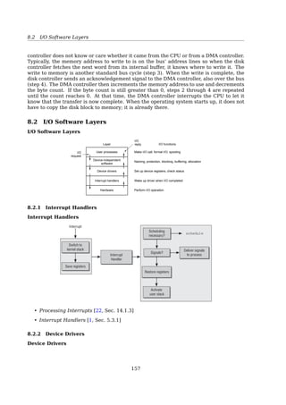
158. 8.1 Principles of I/O Hardware
How can the processor give commands and data to a controller to accomplish an I/O
transfer? The short answer is that the controller has one or more registers for data and
control signals. The processor communicates with the controller by reading and writing
bit patterns in these registers. One way in which this communication can occur is through
the use of special I/O instructions that specify the transfer of a byte or word to an I/O port
address. The I/O instruction triggers bus lines to select the proper device and to move bits
into or out of a device register. Alternatively, the device controller can support memory-
mapped I/O. In this case, the device-control registers are mapped into the address space
of the processor. The CPU executes I/O requests using the standard data-transfer instruc-
tions to read and write the device-control registers. Some systems use both techniques.
For instance, PCs use I/O instructions[17, Sec. 12.2, I/O Hardware].
How do these schemes work? In all cases, when the CPU wants to read a word, either
from memory or from an I/O port, it puts the address it needs on the bus’ address lines and
then asserts a READ signal on a bus’ control line. A second signal line is used to tell whether
I/O space or memory space is needed. If it is memory space, the memory responds to the
request. If it is I/0 space, the I/0 device responds to the request. If there is only memory
space [as in (b)], every memory module and every I/O device compares the address lines
to the range of addresses that it services. If the address falls in its range, it responds to
the request. Since no address is ever assigned to both memory and an I/O device, there
is no ambiguity and no conflict[19, Sec. 5.1.3, Memory-mapped I/O].
Advantages of Memory-mapped I/O
No assembly code is needed (IN, OUT...)
With memory-mapped I/O, device control registers are just variables in memory and can
be addressed in C the same way as any other variables. Thus with memory-mapped I/O, a
I/O device driver can be written entirely in C.
No special protection mechanism is needed
The I/O address space is part of the kernel space, thus cannot be touched directly by any
user space process.
The two schemes for addressing the controllers have different strengths and weak-
nesses. Let us start with the advantages of memory-mapped I/O. First, if special I/0 in-
structions are needed to read and write the device control registers, access to them re-
quires the use of assembly code since there is no way to execute an IN or OUT instruction
in C or C++. Calling such a procedure adds overhead to controlling I/O. In contrast, with
memory-mapped I/O, device control registers are just variables in memory and can be ad-
dressed in C the same way as any other variables. Thus with memory-mapped I/O, a I/O
device driver can be written entirely in C. Without memory-mapped I/O, some assembly
code is needed[19, Sec. 5.1.3, Memory-mapped I/O].
Second, with memory-mapped I/O, no special protection mechanism is needed to keep
user processes from performing I/O. All the operating system has to do is refrain from
putting that portion of the address space containing the control registers in any user’s
virtual address space. Better yet, if each device has its control registers on a different
page of the address space, the operating system can give a user control over specific
devices but not others by simply including the desired pages in its page table. Such a
scheme can allow different device drivers to be placed in different address spaces, not
only reducing kernel size but also keeping one driver from interfering with others.
Third, with memory-mapped I/O, every instruction that can reference memory can also
reference control registers. For example, if there is an instruction, TEST, that tests a mem-
ory word for 0, it can also be used to test a control register for 0, which might be the signal
that the device is idle and can accept a new command. The assembly language code might
look like this:
153

159. 8.1 Principles of I/O Hardware
LOOP: TEST PORT_4 ;check if port 4 is 0
BEQ READY ;if it is 0, go to ready
BRANCH LOOP ;otherwise, continue testing
READY:
If memory-mapped I/O is not present, the control register must first be read into the
CPU, then tested, requiring two instructions instead of one. In the case of the loop given
above, a fourth instruction has to be added, slightly slowing down the responsiveness of
detecting an idle device.
Disadvantages of Memory-mapped I/O
Caching problem
• Caching a device control register would be disastrous
• Selectively disabling caching adds extra complexity to both hardware and the OS
Problem with multiple buses
CPU Memory I/O
Bus
All addresses (memory
and I/O) go here
CPU Memory I/O
CPU reads and writes of memory
go over this high-bandwidth bus
This memory port is
to allow I/O devices
access to memory
(a) (b)
Fig. 5-3. (a) A single-bus architecture. (b) A dual-bus memory
architecture.
Figure 2: (a) A single-bus architecture. (b) A dual-bus memory architecture.
In computer design, practically everything involves trade-offs, and that is the case here
too. Memory-mapped I/O also has its disadvantages. First, most computers nowadays
have some form of caching of memory words. Caching a device control register would be
disastrous. Consider the assembly code loop given above in the presence of caching. The
first reference to PORT_4 would cause it to be cached. Subsequent references would just
take the value from the cache and not even ask the device. Then when the device finally
became ready, the software would have no way of finding out. Instead, the loop would go
on forever[19, Sec. 5.1.3, Memory-mapped I/O].
To prevent this situation with memory-mapped I/O, the hardware has to be equipped
with the ability to selectively disable caching, for example, on a per page basis. This
feature adds extra complexity to both the hardware and the operating system, which has
to manage the selective caching.
Second, if there is only one address space, then all memory modules and all I/O devices
must examine all memory references to see which ones to respond to. If the computer has
a single bus, as in Fig 2(a), having everyone look at every address is straightforward.
However, the trend in modern personal computers is to have a dedicated high-speed
memory bus, as shown in Fig 2(b), a property also found in main-frames, incidentally. This
154

160. 8.1 Principles of I/O Hardware
bus is tailored to optimize memory performance, with no compromises for the sake of slow
I/O devices. Pentium systems can have multiple buses (memory, PCI, SCSI, USB, ISA), as
shown in Fig 3.
ISA
bridge
Modem
Mouse
PCI
bridgeCPU
Main
memory
SCSI USB
Local bus
Sound
card
Printer Available
ISA slot
ISA bus
IDE
disk
Available
PCI slot
Key-
board
Mon-
itor
Graphics
adaptor
Level 2
cache
Cache bus Memory bus
PCI bus
Fig. 1-11. The structure of a large Pentium system
Figure 3: The structure of a large Pentium system
The trouble with having a separate memory bus on memory-mapped machines is that
the I/O devices have no way of seeing memory addresses as they go by on the memory bus,
so they have no way of responding to them. Again, special measures have to be taken to
make memory-mapped I/O work on a system with multiple buses. One possibility is to first
send all memory references to the memory. If the memory fails to respond, then the CPU
tries the other buses. This design can be made to work but requires additional hardware
complexity.
A second possible design is to put a snooping device on the memory bus to pass all
addresses presented to potentially interested I/O devices. The problem here is that I/0
devices may not be able to process requests at the speed the memory can.
A third possible design, which is the one used on the Pentium configuration of Fig 3,
is to filter addresses in the PCI bridge chip. This chip contains range registers that are
preloaded at boot time. For example, 640K to 1M could be marked as a nonmemory range.
Addresses that fall within one of the ranges marked as nonmemory are forwarded onto the
PCI bus instead of to memory. The disadvantage of this scheme is the need for figuring
out at boot time which memory addresses are not really memory addresses. Thus each
scheme has arguments for and against it, so compromises and trade-offs are inevitable.
8.1.1 Programmed I/O
Programmed I/O
Handshaking
155

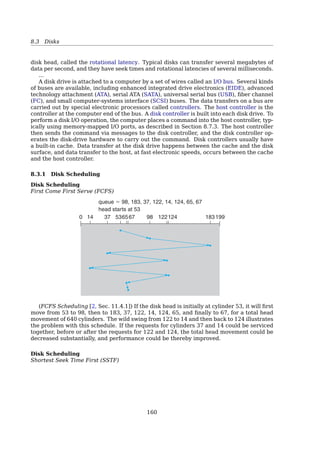
161. 8.1 Principles of I/O Hardware
...........
busy = ?
.
0
.....
write a byte
.....
command-ready = 1
.....
command-ready = ?
.
1
.....
busy = 1
.....
write == 1?
.
1
.....
read
.
1 byte
.....
command-ready = 0, error = 0, busy = 0
.Host:. status:Register. control:Register. data-out:Register. Controller:
For this example, the host writes output through a port, coordinating with the controller
by handshaking as follows[17, Sec. 12.2.1, Polling].
1. The host repeatedly reads the busy bit until that bit becomes clear.
2. The host sets the write bit in the command register and writes a byte into the data-out
register.
3. The host sets the command-ready bit.
4. When the controller notices that the command-ready bit is set, it sets the busy bit.
5. The controller reads the command register and sees the write command. It reads the
data-out register to get the byte and does the I/O to the device.
6. The controller clears the command-ready bit, clears the error bit in the status register
to indicate that the device I/O succeeded, and clears the busy bit to indicate that it
is finished.
This loop is repeated for each byte.
Example
Steps in printing a string
String to
be printedUser
space
Kernel
space
ABCD
EFGH
Printed
page
(a)
ABCD
EFGH
ABCD
EFGH
Printed
page
(b)
A
Next
(c)
AB
Next
Fig. 5-6. Steps in printing a string.
1 copy_from_user(buffer, p, count); /* p is the kernel bufer */
2 for (i = 0; i count; i++) { /* loop on every character */
3 while(*printer_status_reg != READY); /* loop until ready */
4 *printer_data_register = p[i]; /* output one character */
5 }
6 return_to_user();
See also: [19, Sec. 5.2.2, Programmed I/O].
156

162. 8.1 Principles of I/O Hardware
8.1.2 Interrupt-Driven I/O
Pulling Is Inefficient
A better way
Interrupt The controller notifies the CPU when the device is ready for service.
1.2 Computer-System Organization 9
user
process
executing
CPU
I/O interrupt
processing
I/O
request
transfer
done
I/O
request
transfer
done
I/O
device
idle
transferring
Figure 1.3 Interrupt time line for a single process doing output.
the interrupting device. Operating systems as different as Windows and UNIX
dispatch interrupts in this manner.
The interrupt architecture must also save the address of the interrupted
instruction. Many old designs simply stored the interrupt address in a
fixed location or in a location indexed by the device number. More recent
architectures store the return address on the system stack. If the interrupt
routine needs to modify the processor state—for instance, by modifying
register values—it must explicitly save the current state and then restore that
state before returning. After the interrupt is serviced, the saved return address
is loaded into the program counter, and the interrupted computation resumes
as though the interrupt had not occurred.
1.2.2 Storage Structure
The CPU can load instructions only from memory, so any programs to run must
be stored there. General-purpose computers run most of their programs from
rewriteable memory, called main memory (also called random-access memory
or RAM). Main memory commonly is implemented in a semiconductor
technology called dynamic random-access memory (DRAM). Computers use
other forms of memory as well. Because the read-only memory (ROM) cannot
be changed, only static programs are stored there. The immutability of ROM
is of use in game cartridges. EEPROM cannot be changed frequently and so
contains mostly static programs. For example, smartphones have EEPROM to
store their factory-installed programs.
All forms of memory provide an array of words. Each word has its
own address. Interaction is achieved through a sequence of load or store
instructions to specific memory addresses. The load instruction moves a word
from main memory to an internal register within the CPU, whereas the store
instruction moves the content of a register to main memory. Aside from explicit
loads and stores, the CPU automatically loads instructions from main memory
for execution.
A typical instruction–execution cycle, as executed on a system with a von
Neumann architecture, first fetches an instruction from memory and stores
that instruction in the instruction register. The instruction is then decoded
and may cause operands to be fetched from memory and stored in some
See also: [17, Sec. 12.2.2, Interrupts].
Example
Writing a string to the printer using interrupt-driven I/O
When the print system call is made...
1 copy_from_user(buffer, p, count);
2 enable_interrupts();
3 while(*printer_status_reg != READY);
4 *printer_data_register = p[0];
5 scheduler();
Interrupt service procedure for the printer
1 if (count == 0) {
2 unblock_user();
3 } else {
4 *printer_data_register = p[1];
5 count = count - 1;
6 i = i + 1;
7 }
8 acknowledge_interrupt();
9 return_from_interrupt();
See also: [19, Sec. 5.2.3, Interrupt-Driven I/O].
8.1.3 Direct Memory Access (DMA)
Direct Memory Access (DMA)
Programmed I/O (PIO) tying up the CPU full time until all the I/O is done (busy waiting)
Interrupt-Driven I/O an interrupt occurs on every charcater (wastes CPU time)
Direct Memory Access (DMA) Uses a special-purpose processor (DMA controller) to
work with the I/O controller
157

163. 8.1 Principles of I/O Hardware
Example
Printing a string using DMA
In essence, DMA is programmed I/O, only with the DMA controller doing all the work,
instead of the main CPU.
When the print system call is made...
1 copy_from_user(buffer, p, count);
2 set_up_DMA_controller();
3 scheduler();
Interrupt service procedure
1 acknowledge_interrupt();
2 unblock_user();
3 return_from_interrupt();
The big win with DMA is reducing the number of interrupts from one per character to
one per buffer printed.
The operating system can only use DMA if the hardware has a DMA controller, which
most systems do. Sometimes this controller is integrated into disk controllers and other
controllers, but such a design requires a separate DMA controller for each device. More
commonly, a single DMA controller is available (e.g., on the parentboard) for regulating
transfers to multiple devices, often concurrently[19, Sec. 5.1.4, Direct Memory Access
(DMA)].
DMA Handshaking Example
Read from disk
..........
read
.
data
.....
data ready?
.
yes
.....
DMA-request
.......
DMA-acknowledge
...
memory address
.....
data
.Disk:. Disk Controller:. DMA Controller:. Memory:
The DMA controller
• has access to the system bus independent of the CPU
• contains several registers that can be written and read by the CPU. These includes
– a memory address register
– a byte count register
158

164. 8.2 I/O Software Layers
– one or more control registers
* specify the I/O port to use
* the direction of the transfer (read/write)
* the transfer unit (byte/word)
* the number of bytes to transfer in one burst.
CPU
DMA
controller
Disk
controller
Main
memory
Buffer
1. CPU
programs
the DMA
controller
Interrupt when
done
2. DMA requests
transfer to memory 3. Data transferred
Bus
4. Ack
Address
Count
Control
Drive
Fig. 5-4. Operation of a DMA transfer.
When DMA is used, ..., first the CPU programs the DMA controller by setting its regis-
ters so it knows what to transfer where (step 1 in Fig 380). It also issues a command to
the disk controller telling it to read data from the disk into its internal buffer and verify
the checksum. When valid data are in the disk controller’s buffer, DMA can begin[19,
Sec. 5.1.4, Direct Memory Access (DMA)].
The DMA controller initiates the transfer by issuing a read request over the bus to the
disk controller (step 2). This read request looks like any other read request, and the disk
controller does not know or care whether it came from the CPU or from a DMA controller.
Typically, the memory address to write to is on the bus’ address lines so when the disk
controller fetches the next word from its internal buffer, it knows where to write it. The
write to memory is another standard bus cycle (step 3). When the write is complete, the
disk controller sends an acknowledgement signal to the DMA controller, also over the bus
(step 4). The DMA controller then increments the memory address to use and decrements
the byte count. If the byte count is still greater than 0, steps 2 through 4 are repeated
until the count reaches 0. At that time, the DMA controller interrupts the CPU to let it
know that the transfer is now complete. When the operating system starts up, it does not
have to copy the disk block to memory; it is already there.
8.2 I/O Software Layers
I/O Software Layers
I/O
request
Layer
I/O
reply I/O functions
Make I/O call; format I/O; spooling
Naming, protection, blocking, buffering, allocation
Set up device registers; check status
Wake up driver when I/O completed
Perform I/O operation
User processes
Device-independent
software
Device drivers
Interrupt handlers
Hardware
Fig. 5-16. Layers of the I/O system and the main functions of each
layer. 159

165. 8.2 I/O Software Layers
8.2.1 Interrupt Handlers
Interrupt Handlers
Chapter 14: Kernel Activities
mode stack. However, this alone is not sufficient. Because the kernel also uses CPU resources to execute
its code, the entry path must save the current register status of the user application in order to restore it
upon termination of interrupt activities. This is the same mechanism used for context switching during
scheduling. When kernel mode is entered, only part of the complete register set is saved. The kernel does
not use all available registers. Because, for example, no floating point operations are used in kernel code
(only integer calculations are made), there is no need to save the floating point registers.3 Their value
does not change when kernel code is executed. The platform-specific data structure pt_regs that lists all
registers modified in kernel mode is defined to take account of the differences between the various CPUs
(Section 14.1.7 takes a closer look at this). Low-level routines coded in assembly language are responsible
for filling the structure.
Interrupt
Handler
Scheduling
necessary?
Signals?
Restore registers
Deliver signals
to process
Activate
user stack
Switch to
kernel stack
Save registers
Interrupt
schedule
Figure 14-2: Handling an interrupt.
In the exit path the kernel checks whether
❑ the scheduler should select a new process to replace the old process.
❑ there are signals that must be delivered to the process.
Only when these two questions have been answered can the kernel devote itself to completing its regular
tasks after returning from an interrupt; that is, restoring the register set, switching to the user mode
stack, switching to an appropriate processor mode for user applications, or switching to a different
protection ring.4
Because interaction between C and assembly language code is required, particular care must be taken
to correctly design data exchange between the assembly language level and C level. The corresponding
code is located in arch/arch/kernel/entry.S and makes thorough use of the specific characteristics
of the individual processors. For this reason, the contents of this file should be modified as seldom as
possible — and then only with great care.
3Some architectures (e.g., IA-64) do not adhere to this rule but use a few registers from the floating comma set and save them each
time kernel mode is entered. The bulk of the floating point registers remain ‘‘untouched‘‘ by the kernel, and no explicit floating point
operations are used.
4Some processors make this switch automatically without being requested explicitly to do so by the kernel.
851
See also:
• [12, Sec. 14.1.3, Processing Interrupts]
• [19, Sec. 5.3.1, Interrupt Handlers]
8.2.2 Device Drivers
Device Drivers
User
space
Kernel
space
User process
User
program
Rest of the operating system
Printer
driver
Camcorder
driver
CD-ROM
driver
Printer controllerHardware
Devices
Camcorder controller CD-ROM controller
Fig. 5-11. Logical positioning of device drivers. In reality all
communication between drivers and device controllers goes over
the bus.
See also: [19, Sec. 5.3.2, Device Drivers].
160

166. 8.2 I/O Software Layers
8.2.3 Device-Independent I/O Software
Device-Independent I/O Software
Functions
• Uniform interfacing for device drivers
• Buffering
• Error reporting
• Allocating and releasing dedicated devices
• Providing a device-independent block size
See also: [19, Sec. 5.3.3, Device-Independent I/O Software].
Uniform Interfacing for Device Drivers
Operating system Operating system
Disk driver Printer driver Keyboard driver Disk driver Printer driver Keyboard driver
(a) (b)
Fig. 5-13. (a) Without a standard driver interface. (b) With a stan-
dard driver interface.
Buffering
User process
User
space
Kernel
space
2 2
1 1 3
Modem Modem Modem Modem
(a) (b) (c) (d)
Fig. 5-14. (a) Unbuffered input. (b) Buffering in user space.
(c) Buffering in the kernel followed by copying to user space. (d)
Double buffering in the kernel.
8.2.4 User-Space I/O Software
User-Space I/O Software
Examples:
• stdio.h, printf(), scanf()...
• spooling(printing, USENET news...)
See also: [19, Sec. 5.3.4, User-Space I/O Software].
161