Download to read offline

![Chapter 1
Introduction
Transport and mobility plays an important role in nowadays society. In Europe1, the
transport industry directly employs more than 10 million people that corresponds to
4.5% of total employment. When passenger transport2 is considered, more than 6000
billion passenger-kilometres (pkm) are travelled every year with more than 70% pkm
travelled by car. Such a huge amount of travel, however, takes its toll on the en-
vironment. Transport greenhouse gas emissions increased3 by around 34% between
1990 and 2008. Nowadays, transport is responsible for about a quarter of the EU’s
greenhouse gas emissions. In larger cities, drivers spend tens of hours a year in road
traffic jams. In total, congestion costs Europe about 1% of GDP every year4.
In order to alleviate the negative impacts of growing transport, we need to make
transport and mobility sustainable. The World Business Council for Sustainable
Development defines sustainable mobility as “the ability to meet the needs of society
to move freely, gain access, communicate, trade, and establish relationships without
sacrificing other essential human or ecological values today or in the future” [1].
Moving to sustainable transport corresponds to general sustainability goal which is
in Europe proclaimed by the Europe 20205 growth strategy.
Moreover, in addition to transport becoming more intensive, transport systems are
also becoming more complex, offering multitude different ways of travel. Providing
intelligent tools that would help citizens make the best use of mobility services on offer
is thus needed more than ever [92]. The problem of journey planning in transport
networks has been studied for a long time [5]. In principle, majority of techniques
find a shortest path using a graph model of the transport network. Traditionally, the
problem of routing on road networks has been studied since 1960s. In last decades,
1
http://ec.europa.eu/transport/strategies/facts-and-figures/transport-matters/
index_en.htm
2
http://www.eea.europa.eu/data-and-maps/figures/passenger-transport-volume-
billion-pkm-1
3
http://ec.europa.eu/transport/strategies/facts-and-figures/putting-
sustainability-at-the-heart-of-transport/index_en.htm
4
See footnote 1.
5
http://ec.europa.eu/europe2020/index_en.htm
1](https://image.slidesharecdn.com/5227de32-e56f-4573-b73a-9a28ea360750-170109080048/85/dissertation_hrncir_2016_final-9-320.jpg)
![1.1. RESEARCH OBJECTIVES
routing research has focused on more challenging problems of multimodal public
transport routing, intermodal routing, and realistic network modelling (e.g., taking
into account real-time information about public transport vehicles).
Given the proclaimed shift towards sustainable transport and mobility, it is im-
portant that journey planning techniques fully support planning journeys using sus-
tainable modes of transport. Therefore, the aim of the thesis is to develop models
and algorithms that support journey planning for sustainable transport, i.e., plan-
ning journeys from an origin to a destination that respect user preferences and utilise
a combination of sustainable modes of transport. The sustainable modes of transport
include (shared) bike, (shared) electric scooter, shared car, or public transport (PT).
To give just one example, bike is an affordable human-powered mode of transport
that does not need oil-based fuels. Importantly, riding a bicycle has positive health
effects related to regular physical activity and decreased air and noise pollution [115].
1.1 Research Objectives
The high-level objective of the thesis is to design, develop, evaluate, and validate mod-
els and algorithms that would maximally support journey planning for sustainable
transport. We summarise the research objectives into the following items:
1. Formal models. The first objective is to understand the transport network
domain and formalise models that will enable solving the chosen problems of
sustainable journey planning using efficient algorithms. Each of the models
needs to capture the specific features of the chosen problems.
2. Efficient algorithms. The second objective is to design and implement ef-
ficient algorithms that would solve the chosen problems using the models de-
veloped within Research objective 1. The algorithms should have favourable
computational properties allowing them to scale to real-world problem sizes.
The implementation should use memory-efficient data structures, preprocess-
ing, and other low-level enhancements to keep the runtime per query and mem-
ory consumption reasonably low. An inseparable part of this objective is to
evaluate the implemented algorithms using real-world map and PT timetables
data. The algorithms will be evaluated with respect to runtime and quality of
returned plans.
3. Validation in real-world deployments. The third and final objective is to
validate the implemented algorithms within Research objective 2 in real-world
deployments with real users. This objective comprises the full research and
development cycle starting from models and continuing with efficient algorithms
and their evaluation. Through real-world deployments only, it is possible to
discover real issues and the next research directions to achieve a system capable
of real-world operation.
2](https://image.slidesharecdn.com/5227de32-e56f-4573-b73a-9a28ea360750-170109080048/85/dissertation_hrncir_2016_final-10-320.jpg)
![1.2. PROBLEM CLASSIFICATION
1.2 Problem Classification
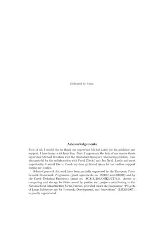
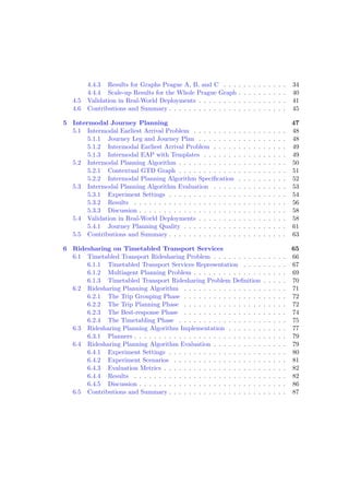
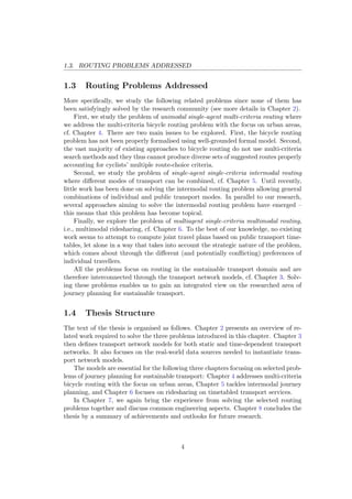
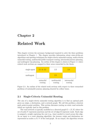
In this thesis, we explore three related problems of sustainable journey planning that
are marked by yellow boxes in Figure 1.1. The problems are classified according
to three dimensions: single-agent vs multiagent, single-criteria vs multi-criteria, and
unimodal vs multimodal vs intermodal routing.
unimodal
routing
intermodal
routing
multiagent
single-agent
multimodal
routing
multi-criteria
(Chapter 4)
single-criteria
(Chapter 6)
single-criteria
(Chapter 5)
Figure 1.1: Problem classification according to three dimensions. Three researched
problems of sustainable journey planning are marked by yellow boxes. References in
brackets point to chapters where the problems are presented in detail.
In the first problem classification dimension, within single-agent problems, there
is just one actor in an environment (e.g., a user of a multimodal journey planner
that requests a journey plan) with no interaction with other actors. In multiagent
problems, the actors interacts with each other in an environment (e.g., they collab-
orate in ridesharing to accomplish their goal of getting to their destinations). The
second problem classification dimension concerns the number of criteria considered
when solving a journey planning problem. Finally, the third problem classification
dimension classifies journey planning problems with respect to number of modes com-
bined in the planner. In unimodal routing, only one mode of transport is handled (for
example the bike in bike planners). In multimodal routing, several public transport
modes are combined (e.g., a public transport planner handling combinations of un-
derground, trams, and buses). In the most complex setting of intermodal routing6,
planners should be able to plan journeys which use a combination of a full range of
transport modes, including scheduled PT (e.g., bus, underground, tram, train, ferry),
individual transport (e.g., walk, bike, shared bike and car), and on-demand transport
(e.g., taxi). We use the term intermodal in order to stress that we consider modes
and combinations thereof that go beyond what is supported in existing multimodal
journey planners.
6
In our previous work [63, 71], we referred to this term as fully multimodal routing. In recent
years, the terminology has evolved and so we now use the term intermodal routing since it has
become a commonly used term in the routing research community.
3](https://image.slidesharecdn.com/5227de32-e56f-4573-b73a-9a28ea360750-170109080048/85/dissertation_hrncir_2016_final-11-320.jpg)
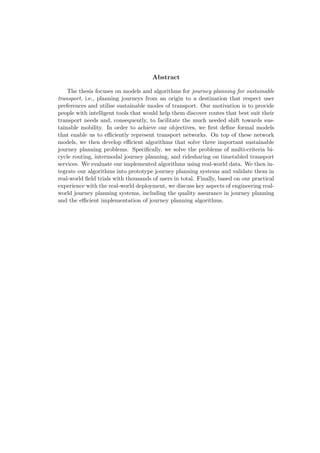
![2.1. SINGLE-CRITERIA UNIMODAL ROUTING
an optimal path, i.e., a sequence of edges, from the origin to the destination node.
An optimal path is the path with the least total cost.
The basic algorithm for finding a shortest point-to-point path is the Dijkstra’s
algorithm [37]. When the Fibonacci heap [46] is used for the priority queue of nodes,
the computational complexity of the Dijkstra’s algorithm is O(|E| + |V | + log |V |).
In practice, the runtimes of the Dijkstra’s algorithm are excessive when a large road
network is used. In order to speedup road routing, the road network graph can be
preprocessed and speedup techniques exploiting the following properties of the road
network can be used [98]:
1. A road network is a very sparse and almost planar graph.
2. A road network has a layout, i.e., geographic coordinates of nodes are known.
3. A road network usually has hierarchical properties (there are for example main
streets and less important ones).
Depending on the size of the transport network, speedup techniques enable an-
swering shortest path queries in a fraction of a second. The most recent algorithms
pushed the average query time to microseconds on the Western Europe graph with
42.5 million directed edges. In the following list, there are examples of specific speedup
techniques that use advanced preprocessing strategies and goal-directed search tech-
niques to exploit the above mentioned properties of road networks.
1. SHARC [8]: A unidirectional hierarchical approach that runs a strongly goal-
directed search on the highest level and automatically level down when getting
close to a goal node.
2. Landmark A* (ALT) [52, 53]: A combination of A* search and a lower-
bounding technique based on landmarks and the triangle inequality.
3. Highway hierarchies [94, 95]: An approach exploiting the natural hierarchy
of road networks that uses a complete bidirectional search. The graph is con-
structed in a way that a local area around an origin and a destination contains
all edges whereas a sparser highway network shortest paths preserving graph is
constructed for the rest of the road network.
4. Contraction hierarchies [50]: This approach is based on the contraction of
the least important nodes. In the algorithm, the shortest paths using a con-
tracted node are replaced by shortcuts.
5. Transit-node routing [6, 7]: Distance table for important transit nodes and
all relevant connections between the other nodes and the transit nodes are
precomputed. Fast table lookups are then used in the shortest path search.
6](https://image.slidesharecdn.com/5227de32-e56f-4573-b73a-9a28ea360750-170109080048/85/dissertation_hrncir_2016_final-14-320.jpg)
![2.2. MULTI-CRITERIA UNIMODAL ROUTING
6. Customisable Route Planning [31]: This algorithm uses arc separators to
build the overlay graph. It is engineered to handle turn costs and fast updates
of the cost function needed by real-world systems operating on road networks.
The preprocessing is therefore divided in two parts: metric-independent and
customisable.
7. Hub Labeling [30]: In the preprocessing, each node in the road graph is
assigned a label. The idea is that for any pair of nodes, the mutual distance
can be calculated only by retrieving label values of the two nodes. The labels
must obey the cover property.
2.2 Multi-Criteria Unimodal Routing
Multi-criteria shortest path problem has been studied in the literature for a long
time [5]. The goal is to find a full Pareto set of routes, i.e., all routes non-dominated
by any other route. It belongs to the category of NP hard problems [47]. The main
parameter that affects the runtime of the algorithm is the size of Pareto set. In
general, the Pareto set can be exponentially large in the input graph size even for
the case of two optimisation criteria [57, 81]. That leads to runtimes that are not
practically usable.
As far as general multi-criteria shortest path algorithms are concerned, the multi-
criteria label-setting (MLS) algorithm [57, 78] extends Dijkstra’s algorithm [37] by
operating on labels that have multiple cost values. For each node, the algorithm
stores a bag of non-dominated labels. The priority queue stores labels (typically
in a lexicographic order) instead of nodes as in Dijkstra’s algorithm. A minimum
label from the priority queue is processed in every iteration. On the contrary, the
multi-criteria label-correcting (MLC) algorithm [25, 34] processes the whole bag of
nondominated labels associated with a current node at once. Therefore, labels may
be scanned multiple times during one run of the algorithm.
To speedup the multi-criteria search, heuristic accelerations have attracted consid-
erable attention, aiming at finding a set of routes that is similar to the optimal Pareto
solution. First, the search space can be pruned using the ellipse around the origin
and destination [56]. Second, in [89], the authors proposed a near admissible multi-
criteria search algorithm to approximate the optimal set of Pareto routes in a state
space graph by using the -dominance approach. It has been proven that the (1+ )-
Pareto sets have a polynomial size [88]. Third, in [27], the authors developed several
heuristics to weaken the domination rules during the search (e.g., using buckets for
the criteria values). Fourth, in [55], the authors proposed a modified label-correcting
algorithm with a new label-selection strategy and dominance conditions.
An alternative approach is represented by MOA* [104] and NAMOA* [77] that
are multi-criteria extensions of the standard A* algorithm [58]. The extension lies in
using a vector of heuristics and a search graph, i.e., a directed acyclic graph to record
the set of non-dominated paths to visited nodes. Every time a new path reaches a
node, its cost vector is checked for dominance with the set of all stored path cost
7](https://image.slidesharecdn.com/5227de32-e56f-4573-b73a-9a28ea360750-170109080048/85/dissertation_hrncir_2016_final-15-320.jpg)
![2.3. MULTIMODAL PUBLIC TRANSPORT ROUTING
vectors at that node. The NAMOA* algorithm with the Tung & Chew heuristic [111]
was recently shown to achieve an order of magnitude speedup for bicriteria road
routing [76].
Since the thesis deals with the multi-criteria bicycle routing problem, we dedi-
cate the rest of this section to the overview of search algorithms related to bicycle
routing. In contrast to car and public transport route planning for which advanced
algorithms and mature software implementations exist [5], bicycle routing is a rela-
tively underexplored topic. In particular, despite the highly multi-criteria nature of
cyclists’ route-choice preferences, almost all existing approaches to bicycle routing do
not use multi-criteria search methods to properly account for such a multi-criteriality.
Instead, these existing bicycle routing approaches transform multi-criteria search to
single-criterion search either by optimising each criteria separately [59, 107] or by
using a weighted combination of all criteria [66, 112].
Unfortunately, the scalarisation of multi-criteria problems using a linear combi-
nation of criteria may miss many Pareto optimal routes [21, 26] and consequently
reduce the quality and relevance of suggested routes. Scalarisation also requires the
user to weight the importance of individual route criteria a priori, which is difficult
for most users.
On the way to the multi-criteria search, there is an approach by Storandt [105]
that solves a constrained shortest path problem in the bicycle routing domain. They
solve two problems: (1) Find the route from an origin to a destination with the least
(positive) height difference (summed over all segments) which has length at most D;
(2) Find the route from an origin to a destination which is shortest among all paths
which have height difference of at most H.
Only in the last few years, multi-criteria algorithms for bicycle routing started
to appear. In [96], the authors showed how to effectively search for a best compro-
mise solution in bicycle routing. However, the method only uses two optimisation
criteria and it does not produce multiple solutions approximating the full Pareto set.
Recently, in [103], we have explored the use of optimal multi-criteria shortest path
algorithms for tri-criteria bicycle routing; however, the proposed algorithm is too slow
for interactive route planning.
2.3 Multimodal Public Transport Routing
The aim of an algorithm for planning with scheduled PT services is to find an optimal
journey(s) given an origin, a destination, time constraints, and PT timetables. The
most important difference to road networks discussed in Section 2.1 is the inherent
time dependence of the PT network because PT edges can be traversed only at
specific, discrete times. We begin with the models used to model the PT network
and continue with problem variants and possible solutions.
There are two major ways to model PT timetables for the planning algorithm as
a search graph. On the one hand, in the time-expanded approach [100], each event at
a PT station, e.g., the departure of a train, is modelled as a node in the graph. The
8](https://image.slidesharecdn.com/5227de32-e56f-4573-b73a-9a28ea360750-170109080048/85/dissertation_hrncir_2016_final-16-320.jpg)
![2.3. MULTIMODAL PUBLIC TRANSPORT ROUTING
advantage of this approach is that it allows more-or-less straightforward modelling of
model extensions (e.g., vehicle changes). On the other hand, in the time-dependent
approach [15], the graph contains only one node for each station. Some experimental
studies of the two approaches [9, 90] show that the time-dependent approach exhibits
better performance than the time-expanded approach.
In this overview, we focus on two variants of the problem. To begin with, the
earliest arrival problem (EAP) is defined as follows. Given an origin PT stop po,
a destination PT stop pd, and a departure time τ, find a journey that departs from
po no earlier than τ and has the earliest possible arrival to pd. The EAP problem can
be answered in a straightforward way by Dijkstra’s algorithm both using the time-
dependent model (time-dependent Dijkstra, TDD, [19, 40]) and the time-expanded
model (time-expanded Dijkstra, TED, [100]).
To speedup the search, we need to use more advanced techniques but we need
to take into account that PT networks have different structural properties than road
networks [2]. Because of this fact, some of the speedup techniques for road routing
can be modified to solve the EAP while other speedup techniques cannot. In the
following list, we present speedup techniques that solve the EAP.
• SHARC [8]: A modification of the technique used for road routing, cf. Sec-
tion 2.1.
• Contraction Hierarchies [48]: A modification of the techniques used for road
routing, cf. Section 2.1.
• Core-ALT [87]: A combination of ALT and core-based routing, where the core
contains non-contracted time-dependent scheduled PT services while the roads
are contracted.
• Multi-level graph approach [99, 101]: A hierarchical decomposition of a plan-
ning graph to multiple levels. Based on the node separators, the graph is de-
composed to significantly smaller graphs that preserve shortest paths.
• Access-node routing [32]: Inspired by transit-node routing, table lookups are
used in the multimodal shortest path search.
• Accelerated Connection Scan Algorithm [106]: An accelerated version of
connection scan algorithm [35] based on the ideas used in customisable route
planning [31].
In multimodal PT routing, additional criteria such as number of transfers, walking
distance, or price are also important for the travellers. This leads to the multi-criteria
problem which is defined as follows. Given an origin PT stop po, a destination PT
stop pd, and a departure time τ, find a Pareto set of non-dominating journeys with
respect to the optimisation criteria that departs from po no earlier than τ. In the
following list, we present techniques that solves the multimodal multi-criteria routing
problem.
9](https://image.slidesharecdn.com/5227de32-e56f-4573-b73a-9a28ea360750-170109080048/85/dissertation_hrncir_2016_final-17-320.jpg)
![2.4. INTERMODAL JOURNEY PLANNING
• Layered Dijkstra [15, 91]: Using the Dijkstra’s algorithm [37], it finds a Pareto
set of routes optimised with respect to travel time and number of transfers.
It uses a timetable graph copied into K layers where K equals to the maximum
number of transfers.
• Multi-criteria Label-setting (MLS) Algorithm [80, 91]: This algorithm
extends Dijkstra’s algorithm [37] by operating on labels that have multiple cost
values. For more details see Section 2.2.
• Transfer patterns [4, 49]: A transfer pattern is the origin stop, the sequence
of transfers, and the destination stop. The transfer patterns for pairs of stops
are precomputed and then instantiated for a given departure time.
• RAPTOR (Round-bAsed Public Transit Optimised Router) [33]: An
approach targeted specifically for PT networks which is not based on Dijkstra’s
algorithm and uses arrays of trips and routes1 instead of a graph. The algorithm
operates in rounds (one for each PT transfer) and computes arrival times by
traversing every route at most once per round.
• Public Transit Labeling [28]: An approach that reuses ideas from Hub La-
beling road network speedup [30] and applies them to the time-expanded model
of PT network.
2.4 Intermodal Journey Planning
The aim of the algorithm for intermodal journey planning is given an origin, a des-
tination, and time constraints to find an optimal multi-leg journey(s) which can use
any reasonable combination of these modes of transport: fixed-schedule PT modes
(e.g., bus, underground, tram, train, ferry), fixed-station free-floating modes (e.g.,
shared bikes), and unrestricted free-floating modes (e.g., walk, bike, car, taxi). The
most important difference to fixed-schedule PT networks discussed in Section 2.3 is
that the intermodal network consists of parts with different properties (e.g., static
bicycle transport network compared to the time-dependent PT network).
Until recently, very little work has been done to tackle this general problem. One
of few exceptions is the planner proposed by Horn [61] which supports combinations
of scheduled PT and on-demand transport services. The planner is able to construct
a multi-leg journey plan which can combine on-demand and scheduled PT transport.
A limitation of the approach is that the on-demand mode in the multi-leg journey
plan is restricted to the first or last non-walk leg of a journey, i.e., the on-demand
mode serve as a feeder service. The second attempt at solving the intermodal EAP is
provided by Yu and Lu [117] who use a genetic algorithm to construct the sequence
of transport modes in a journey plan. In their experiments, Yu and Lu permit walk,
1
Route is a group of trips (vehicle journeys) that are known to public by the same route number
identifier.
10](https://image.slidesharecdn.com/5227de32-e56f-4573-b73a-9a28ea360750-170109080048/85/dissertation_hrncir_2016_final-18-320.jpg)
![2.5. MULTIAGENT TRIP PLANNING
bus, underground, and taxi modes. However, the individual modes of transport (bike,
shared bike and car) are not used.
Very recently, in parallel to our research, several approaches tackling the inter-
modal journey planning problem have emerged. This is a sign that this problem
has become a significant topic of current importance. To start with, Bast et al. [3]
have used MLS algorithm and contraction to find meaningful combinations of walk-
ing, PT, and car or taxi. They also propose a filtering procedure called “types and
thresholds” to produce a small representative subset of the full Pareto set of solu-
tions. Adding bike as supported mode of transport, Delling et al. [27] have proposed
multimodal multi-criteria RAPTOR (MCR) algorithm to tackle the problem. To
solve the subproblems in PT and road network, the MCR uses RAPTOR and MLS,
respectively. Adding shared (rental) bike and shared (rental) car to the network,
Kirchler has extended the ALT speedup technique [52, 53] to State Dependent ALT
(SDALT) technique [73]. In the preprocessing phase, landmarks are created to bound
the search space. Dibbelt et al. [36] focus on the problem of finding intermodal
journeys that can be constrained by arbitrary user-specified modal sequences. They
build on contraction hierarchies [50] speedup technique and propose user-constrained
contraction hierarchies (UCCH) algorithm. Finally, Gundling et al. [54] solve the
problem of finding a journey with a PT backbone and private mode (walk, car, bike,
and taxi) first and last mile. They address travel time, travel cost, and convenience
as optimisation criteria.
2.5 Multiagent Trip Planning
Automated planning technology [51] has developed a variety of scalable heuristic algo-
rithms for tackling hard planning problems, where plans, i.e., sequences of actions that
achieve a given goal from a given initial state, are calculated by domain-independent
problem solvers. Unlike other approaches to route planning and ridesharing, au-
tomated planning techniques permit a fairly straightforward formalisation of travel
domains, and allow us to capture the joint action space and complex cost landscape
resulting from travellers’ concurrent activities. In terms of algorithmic complexity, the
kind of multiagent planning needed to compute ridesharing plans for several agents
is significantly harder than single-agent planning for two reasons: Firstly, the ability
of each agent to execute actions concurrently [11] may result in exponentially large
sets of actions available in each step in the worst case. Secondly, whenever indi-
vidual agents have different (and potentially conflicting) goals [13], a joint solution
must satisfy additional requirements, e.g., being compatible with everyone’s individ-
ual preferences, or not providing any incentive for any individual to deviate from the
joint plan. Solving the general multiagent planning for problem sizes of the scale
we are interested in real-world ridesharing is therefore not currently possible using
existing techniques.
Because of the desire to integrate different travellers’ individual plans, ridesharing
is quite similar to plan merging (e.g., [45, 110], where individual agents’ plans are in-
11](https://image.slidesharecdn.com/5227de32-e56f-4573-b73a-9a28ea360750-170109080048/85/dissertation_hrncir_2016_final-19-320.jpg)
![2.5. MULTIAGENT TRIP PLANNING
crementally integrated into a joint solution. Compared to these approaches, however,
in our domain every agent can always achieve their plan regardless of what others
do, and agents do not require others’ “help” to achieve their goals. This makes the
problem simpler than those of plan merging though, in return, we place much higher
scalability demands on the respective solution algorithms.
This explains also why, as will be shown below, we are able to achieve much higher
scalability than state-of-the-art multiagent plan synthesis algorithms, e.g., [38, 82,
109]. These algorithms exploit “locality” in different ways in order to be able to
plan for parts of a multiagent planning problem while temporarily ignoring others,
e.g., by considering non-interacting subplans in isolation from each other. In a sense,
our problem involves even more loosely coupled sub-tasks, as these can be essentially
solved in a completely independent way, except in terms of cost optimisation.
The relationship between our work and approaches that focus more on decen-
tralised planning, plan co-ordination, and conflict resolution among independent plan-
ning agents (e.g., [22, 23]) is similar – as no hard conflicts can arise among individual
plans in ridesharing, it is not essential to co-ordinate individual plans with each other,
other than for cost optimisation purposes.
Finally, as far as the strategic aspect is concerned, this is obviously also relevant
to ridesharing as ultimately each co-traveller wants to achieve an optimal solution
for themselves. Various approaches have studied this problem in the past (e.g., [13,
41, 113], yet none of them has been shown to scale to the type of domain we are
interested in, with the exception of [72], which makes certain simplifying assumptions
to achieve scalability: it does not consider joint deviation from equilibrium solutions
(i.e., it only safeguards against individual agents opting out of a joint plan, not
whole sub-groups of agents), and it assumes that agents will honour their promises
when they have agreed on a joint plan. We believe that both these assumptions are
reasonable in ridesharing, as we are envisioning a platform on which users would be
automatically grouped together whenever a rideshare would be beneficial to each one
of them. On such a platform, it is reasonable to assume that agreements could be
enforced through a trusted third party, and that collusion among travellers could be
avoided by not disclosing their identities to each other until the purchase of all tickets
has been completed.
Ridesharing, i.e., purposeful and explicit planning to create groups of people that
travel together in a single vehicle for parts of the journey, is a long known and widely
studied problem. It solves the problem in a multiagent way compared to approaches
that mitigates the negative impacts of the transport on the individual level. Exist-
ing work, however, focuses exclusively on ridesharing using vehicles that can move
freely on a road transport network, without schedule or route restrictions. The work
on such non-timetabled ridesharing covers the whole spectrum from formal problem
models, through solution algorithms up to practical consumer-oriented services and
applications.
On the theoretical side, the vehicle-based ridesharing problem is typically for-
malised as a Dial-a-Ride Problem (DARP). Different variants of DARPs exist, differ-
12](https://image.slidesharecdn.com/5227de32-e56f-4573-b73a-9a28ea360750-170109080048/85/dissertation_hrncir_2016_final-20-320.jpg)
![2.5. MULTIAGENT TRIP PLANNING
ing, for example, in the nature of traveller’s constraints, the distribution of pickup and
delivery locations, the criteria optimised, or the level of dynamism supported. A com-
prehensive review of different variants of DARPs, along with a list of algorithmic
solution approaches, is given by Cordeau et al. [20]. Most of the existing approaches
rely on a centralised coordination entity responsible for collecting requests and pro-
ducing vehicle assignment and schedules, though more decentralised approaches have
also been presented more recently [116]. Bergbelia et al. [10] summarise recent ad-
vances in real-time ridesharing, which has been gaining prominence with the growing
penetration of internet-connected smartphones and GPS-enabled vehicle localisation
technologies. Existing work almost exclusively considers a single mode of transport
only. One of few exceptions is the work of Horn et al. [60] which considers demand-
responsive ridesharing in the context of flexible, multimodal transport systems; the
actual ridesharing is, however, only supported for demand-responsive non-timetabled
journey legs. On the practical side, there exist various online services for car rideshar-
ing2,3 as well as services which assist users in negotiating shared journeys4.
So although both ridesharing using freely moving vehicle and single-agent journey
planning for timetabled services have been extensively studied, the combination of
both, i.e., ridesharing on timetabled services, has not been – to the best of our
knowledge – studied before.
2
https://liftshare.com/
3
https://www.enterprisecarclub.co.uk/
4
http://www.travbuddy.com/
13](https://image.slidesharecdn.com/5227de32-e56f-4573-b73a-9a28ea360750-170109080048/85/dissertation_hrncir_2016_final-21-320.jpg)
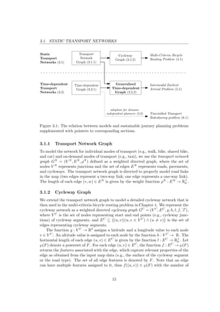
![3.2. TIME-DEPENDENT TRANSPORT NETWORKS
elements |f((u, v))| ≥ 1.
The cost of each edge is calculated by a k-dimensional vector of cost functions
−→c = (c1, c2, . . . , ck). The non-negative cost value ci((u, v)) of i-th criterion for a given
edge (u, v) ∈ E is computed by the cost function ci : EC → R+
0 .
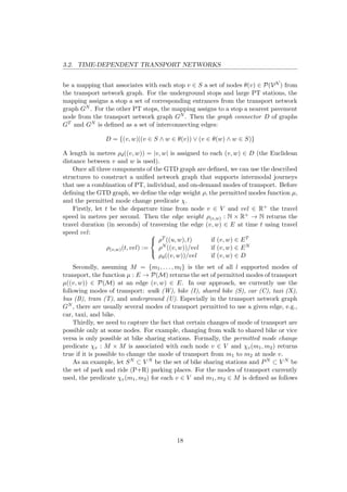
3.2 Time-dependent Transport Networks
In this section, we describe models for the time-dependent transport networks where
the cost of each edge depends on the departure time. We start with a definition of
a time-dependent graph with constant transfer times. Next, we combine this model
with the transport network graph in a novel generalised time-dependent graph that
is able to capture an intermodal transport network.
3.2.1 Time-dependent Graph
To model the network of scheduled PT services (e.g., bus, tram, underground), we
use a time-dependent graph GT = (V T , ET , ρT ) with constant transfer times [91] (the
time needed to make a transfer between two lines at a stop is defined as a constant
for each stop). We have chosen this model for its better performance than the time-
expanded model [90]. Let S be the set of stop nodes corresponding to the stops that
are physically present in the PT network. A stop node can be served by one or more
routes. A route is a set of PT vehicle trips that are known to the public under the
same route number identifier, e.g., the tram line number 3. Assuming that n is the
number of routes using a stop u ∈ S, then n route nodes Ru = {ru
1 , . . . , ru
n}, one
for each route, are associated with stop u. Route nodes are virtual nodes without
corresponding counterparts in the real world and they are used to model constant
transfer times. Without route nodes, it would not be possible to model non-zero
transfer times between different routes at the same stop. The set of all route nodes
is denoted as R = ∪u∈SRu. The set of nodes V T of the time-dependent graph GT is
then defined as V T = S ∪ R.
The set of edges ET of the time-dependent graph GT is defined as ET = A∪B∪C
where A denotes the set of edges between route and stop nodes, B denotes the set of
edges between stop and route nodes, and C denotes the set of route edges between
route nodes of the same route. Edges (v, w) ∈ A ∪ B are called transfer edges.
Formally, the sets are defined as follows:
A = ∪u∈S{(ru, u)|ru ∈ Ru}
B = ∪u∈S{(u, ru)|ru ∈ Ru}
C = ∪u,v∈S{(ru, rv)|ru ∈ Ru ∧ rv ∈ Rv} where ru
and rv are visited successively by the same route
The link-traversal function f (v,w) : N → N is associated with each edge (v, w) ∈ C
and defined as f (v,w)(t) := t where t is the departure time from v and t ≥ t is the
earliest possible arrival time at stop w. We assume that overtaking of vehicles on
16](https://image.slidesharecdn.com/5227de32-e56f-4573-b73a-9a28ea360750-170109080048/85/dissertation_hrncir_2016_final-24-320.jpg)
![3.2. TIME-DEPENDENT TRANSPORT NETWORKS
edges of the same route is not permitted. This means that the earliest arrival of a PT
vehicle to a route node rw
j corresponds to the earliest departure from an adjacent
departure route node rv
i .
Let the function gv return the constant transfer time at stop v. For example in
Figure 3.3, the transfer from a route node rv
0 to rv
1 and vice versa takes time gv. Then
the travel duration ρT
(v,w) : N → N of traversing an edge (v, w) ∈ ET from v at the
departure time t is defined as
ρT
(v,w)(t) :=
0 if (v, w) ∈ A
gv if (v, w) ∈ B
f (v,w)(t) − t if (v, w) ∈ C
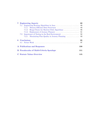
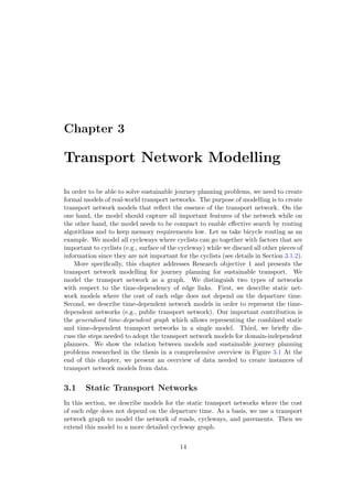
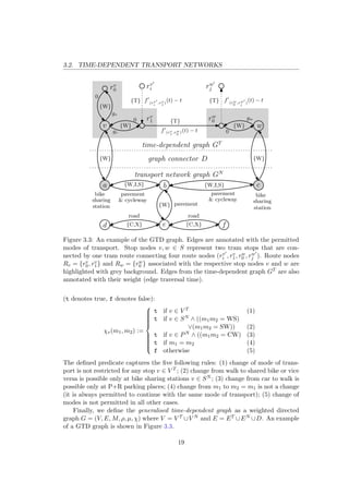
3.2.2 Generalised Time-dependent Graph
In this section, we define the newly proposed generalised time-dependent (GTD)
graph, which allows representing the combined road network (for individual and on-
demand modes) and PT network (for PT modes) in a single structure. The GTD
graph is then used for the intermodal journey planning in Chapter 5.
The GTD graph is a generalisation of the time-dependent graph with constant
transfer times defined by Pyrga et al. [91]. The GTD graph G is constructed from
the following three structures (see also Figure 3.2):
1. transport network graph GN for the network of pavements, cycleways, and roads
(defined in Section 3.1.1)
2. time-dependent graph GT for the PT network (defined in Section 3.2.1)
3. graph connector D of the time-dependent graph GT and the transport network
graph GN (defined below)
Graph Connector. In order to plan multimodal journeys using combinations of
individual, on-demand, and PT modes of transport, the time-dependent graph GT
and the transport network graph GN need to be interconnected. Let θ : S → P(VN )
GTD graph G
transport network
graph GN
time-dependent
graph GT
u ∈ V T v ∈ V N(u, v) ∈ D
(v, u) ∈ D
connector D
graph
Figure 3.2: The structure of a GTD graph.
17](https://image.slidesharecdn.com/5227de32-e56f-4573-b73a-9a28ea360750-170109080048/85/dissertation_hrncir_2016_final-25-320.jpg)
![Chapter 4
Multi-Criteria Bicycle Routing
Increasing the adoption of cycling is crucial for achieving more sustainable urban
mobility since bicycle provides a convenient and affordable form of transport for most
segments of the population. It has a range of health, environmental, economical,
and societal benefits and is therefore promoted as a modern, sustainable mode of
transport [39, 70]. Navigating larger cities on a bicycle is, however, often challenging
due to cities’ fragmented cycling infrastructure or complex terrain topology. Cyclists
would thus benefit from intelligent route planning that would help them discover
routes that best suit their transport needs and preferences.
The first problem addressed in this thesis is the unimodal single-agent multi-
criteria routing. Following the motivation above, we opted to study the multi-criteria
bicycle routing problem with the focus on urban areas. In contrast to car drivers,
cyclists consider a significantly broader range of factors while deciding on their routes.
By employing questionnaires and GPS tracking, researchers have found that besides
travel time and distance, cyclists are sensitive to traffic volumes, junction control, turn
frequency, slope, noise, pollution, and scenery [14, 114]. Because of the many factors
cyclists consider in deciding their routes, employing multi-criteria route search is
vital for properly accounting for cyclists’ route-choice criteria. Moreover, the relative
importance of these factors varies among cyclists and can also be affected by weather
and the purpose of the trip [14]. Such a user- and context-dependent multi-criteriality
makes bicycle routing a particularly difficult category of routing problems. Bicycle
route planner would be particularly useful for inexperienced cyclists with limited
knowledge of their surroundings but they would also benefit experienced riders who
want to fine-tune their routes [43], in effect making cycling a more attractive and
accessible transport option.
The vast majority of existing approaches to bicycle routing, however, do not use
multi-criteria search methods and they thus cannot produce diverse sets of suggested
routes properly accounting for cyclists’ multiple route-choice criteria. In this thesis,
we overcome these limitations and present a bicycle routing algorithm that prop-
erly considers multiple realistic cyclists’ route-choice criteria yet is fast enough for
interactive use. Our algorithm extends the well-known multi-criteria label-setting
22](https://image.slidesharecdn.com/5227de32-e56f-4573-b73a-9a28ea360750-170109080048/85/dissertation_hrncir_2016_final-30-320.jpg)
![4.1. MULTI-CRITERIA BICYCLE ROUTING PROBLEM
algorithm [78] with several speedup heuristics in order to generate, in a much shorter
time, routes that closely approximate the full set of Pareto optimal routes. In con-
trast to the majority of existing work, our algorithm employs a formulation of the
multi-criteria bicycle routing problem that incorporates realistic route choice factors
based on recent studies of cyclists’ behaviour [14, 114]. We thoroughly evaluate our
algorithm in terms of the speed and quality of suggested routes on a diverse set of
real-world urban areas. Finally, we validate the algorithm in real-world deployments
using a bicycle routing system with an open API.
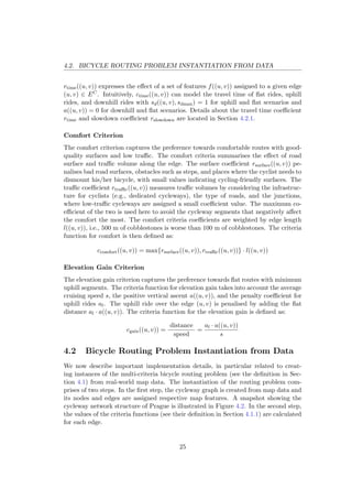
4.1 Multi-Criteria Bicycle Routing Problem
The multi-criteria bicycle routing problem is defined as a triple C = (GC, o, d):
• GC = (V C, EC, g, h, l, f, −→c ) is the cycleway graph (defined in Section 3.1.2)
• o ∈ V C is the route origin
• d ∈ V C is the route destination
A route π, i.e., a finite path π = ((u1, v1), . . . , (un, vn)) with a length |π| = n from
the origin o to the destination d in the cycleway graph GC has an additive cost value:
−→c (π) =
|π|
j=1
c1(uj, vj), . . . ,
|π|
j=1
ck(uj, vj)
The solution of the multi-criteria bicycle routing problem is a full Pareto set of routes
Π ⊆ {π|π = ((u1, v1), . . . , (un, vn))}, i.e., all routes non-dominated by any other
route. A route πp dominates another route πq, i.e., πp πq, iff ci(πp) ≤ ci(πq) for all
1 ≤ i ≤ k and cj(πp) < cj(πq) for at least one j, 1 ≤ j ≤ k.
4.1.1 Tri-Criteria Bicycle Routing Problem
Based on the studies of real-world cycle route choice behaviour [14, 114], we further
consider a specific class of multi-criteria bicycle routing problems – a tri-criteria
bicycle routing problem. Specifically, we consider the travel time criterion ctime, the
comfort criterion ccomfort, and the elevation gain criterion cgain defined in the next
subsections. The criteria functions are then instantiated in Section 4.2.1.
Travel Time Criterion
The travel time criterion captures the preference towards routes that can be travelled
in a short time. Travel time is a sensitive factor in cyclists’ route planning especially
for commuting purposes. To model the slowdown caused by obstacle features such as
stairs or crossings, we define the slowdown coefficient rslowdown : ℘(F) → R+
0 which
returns the slowdown in seconds on the given edge (u, v) ∈ EC with a set of features
f((u, v)).
23](https://image.slidesharecdn.com/5227de32-e56f-4573-b73a-9a28ea360750-170109080048/85/dissertation_hrncir_2016_final-31-320.jpg)
![4.1. MULTI-CRITERIA BICYCLE ROUTING PROBLEM
l((u, v))
h(u)
h(v)
a((u, v))
(a) uphill
l((u, v))
h(u)
h(v)
d((u, v))
(b) downhill
u uv v
Figure 4.1: Positive vertical (a) ascent a and (b) descent d.
Besides, changes in elevation may affect the cyclist’s velocity and hence affect
travel times. For the case of uphill rides, we define the positive vertical ascent a :
EC → R+
0 , cf. Figure 4.1.
a((u, v)) :=
h(v) − h(u) if h(v) > h(u)
0 otherwise
Analogously, for the case of downhill rides, we define the positive vertical descent
d : EC → R+
0 (cf. Figure 4.1) and the positive descent grade d : EC → R+
0 for a
given edge (u, v) ∈ EC as follows:
d((u, v)) :=
h(u) − h(v) if h(u) > h(v)
0 otherwise
d ((u, v)) :=
d((u, v))
l((u, v))
To model the speed acceleration caused by vertical descent for a given edge (u, v) ∈
EC, we define the downhill speed multiplier sd : EC × R+ → R+ as:
sd((u, v), sdmax) :=
sdmax if d ((u, v)) > d c
(sdmax−1)d ((u,v))
d c
+ 1 otherwise
where sdmax ∈ R+ is the maximum downhill speed multiplier, and d c ∈ R+ is the
critical d value over which a downhill ride would use the multiplier of sdmax. This
reflects the fact that the speed acceleration is remarkable for the ride on a steep
downhill (compared to a mild one), however, it is limited due to safety concerns,
bicycle physical limits and air drag.
Considering the integrated effect of edge length, the change in elevation and its
associated features, the travel time criterion is defined as:
ctime((u, v)) =
distance
speed
+ slowdown =
=
l((u, v)) + al · a((u, v))
s · sd((u, v), sdmax) · rtime((u, v))
+ rslowdown((u, v))
where s is the average cruising speed of a cyclist. al is the penalty coefficient for
uphill rides (we use a modification of the Naismith’s rule [97]). The criteria coefficient
24](https://image.slidesharecdn.com/5227de32-e56f-4573-b73a-9a28ea360750-170109080048/85/dissertation_hrncir_2016_final-32-320.jpg)

![4.3. HEURISTIC-ENABLED MULTI-CRITERIA LABEL-SETTING
ALGORITHM
4.3 Heuristic-Enabled Multi-Criteria Label-Setting Al-
gorithm
Our newly proposed heuristic-enabled multi-criteria label-setting (HMLS) algorithm
extends the standard multi-criteria label-setting (MLS) algorithm [78] with several
points for inserting speedup heuristic logic. The algorithm uses the following data
structures: for each node u ∈ V C, L(u) := (u, (l1(u), l2(u), . . . , lk(u)), LP (u)) rep-
resents one of the labels at a node u, which is composed of the node u, the cost
vector l(u) = (l1(u), l2(u), . . . , lk(u)) indicating the current cost values from the ori-
gin to the node u, and the predecessor label LP (u), which precedes L(u) in an optimal
route from an origin. A priority queue Q is used to maintain all labels created dur-
ing the search. Since each node may be scanned multiple times, we define the bag
structure Bag(u) for each node u to maintain the non-dominated labels at u.
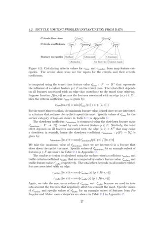
The pseudocode of the heuristic-enabled MLS algorithm is given in Algorithm 1.
The speedups of the MLS algorithm can be implemented using up to three speedup-
specific functions provided by the Heuristic interface: Heuristic.termination-
Condition, Heuristic.skipEdge, and Heuristic.checkDominance. The logic
of the speedup functions is described in Section 4.3.1. Here we describe the overall
heuristic-independent logic which consists of the following steps:
Step 1 – Initialisation: For a k-criteria optimisation problem, the algorithm first
initialises the priority queue Q and Bag for each v ∈ V C. Then it initialises the
label at the origin to L(o) := (o, (l1(o), l2(o), . . . , lk(o)), null), where li(o) = 0 for
i = 1, 2, . . . , k. Finally, it inserts the initial label L(o) into the queue Q and the
Bag(o).
Step 2 – Label expansion: The algorithm extracts a minimum label current :=
(u, (l1(u), l2(u), . . . , lk(u)), LP (u)) from the priority queue Q (in a lexicographic order
of a cost vector). For each outgoing edge (u, v), the algorithm compute new cost
vector (l1(v), l2(v), . . . , lk(v)) by adding the costs of the edge (u, v) to the current
cost values (l1(u), l2(u), . . . , lk(u)). Then, it creates a new label next using the node
v, the cost vector (l1(v), l2(v), . . . , lk(v)) and the predecessor label current.
Function MLS.skipEdge (cf. line 17 of Algorithm 1) prevents looping the path
by checking the predecessor label in the label data structure, i.e., if previous node
LP (u).getNode() is equal to the node v then the edge (u, v) is skipped. We have also
experimented with checking the whole path for cycles. However, this significantly
degraded the runtime of the algorithm. Therefore, we only check the predecessor
label and cycles with larger size are eliminated through dominance checks.
Function MLS.checkDominance (cf. lines 20–23 of Algorithm 1 and Algo-
rithm 6 in Appendix B), by default, controls dominance between the label next and
all labels inside Bag(v). If next is not dominated, the algorithm inserts it into Bag(v)
and Q. Also, if some label inside Bag(v) is dominated by next, it is eliminated from
the bag structure Bag(v) and the priority queue Q, i.e., it will not be considered in
future search.
28](https://image.slidesharecdn.com/5227de32-e56f-4573-b73a-9a28ea360750-170109080048/85/dissertation_hrncir_2016_final-36-320.jpg)
![4.3. HMLS ALGORITHM
Step 3 – Pruning condition: The algorithm exits if the queue Q becomes empty.
Otherwise, it continues with Step 2.
After the algorithm has finished, the optimal Pareto set of routes Π∗ is extracted.
Let |Bag(d)| = |Π| = m. Then, from labels L1, . . . , Lm in the destination Pareto set of
labels Bag(d), the routes π1, . . . , πm are extracted using the predecessor labels LP (·)
(see the pseudocode of extractRoutes method in Algorithm 5 of Appendix B).
These routes comprise the set Π∗ = {π1, π2, . . . , πm} of optimal Pareto routes.
4.3.1 Speedups for the HMLS Algorithm
A significant drawback of the standard MLS algorithm is that it is very slow. The
main parameter that affects the runtime of the algorithm is the size of the Pareto
set. In general, the Pareto set can be exponentially large in the input graph size [81].
Furthermore, the MLS algorithm always explores the whole cycleway graph.
To accelerate the multi-criteria shortest path search, we introduce five speedup
heuristics. Two of the heuristics are newly proposed by us: ratio-based pruning and
cost-based pruning, while three are existing heuristics: ellipse pruning, -dominance
and buckets. Implementation-wise, the heuristics are incorporated into the heuristic-
enabled MLS algorithm by defining the respective three heuristic-specific functions
used in Algorithm 1.
Ellipse Pruning
The first speedup heuristic taken from [56] prevents the MLS algorithm from always
searching the whole cycleway graph, even for a short origin-destination distance1.
The heuristic permits visiting only the nodes that are within a predefined ellipse.
The focal points of the ellipse correspond to the journey origin o and the destination
d. We maintain a constant ratio a
b between semimajor axis a and semiminor axis b. In
addition, to improve the ellipse performance for short origin-destination distances, we
keep a minimum value d min for the length of d = |op| which is the distance between
the origin o and a peripheral point p on the main axis of the ellipse, cf. Figure 4.4.
During the search, in the Ellipse.skipEdge function (cf. Algorithm 1, line 17), it
is checked whether an edge (u, v) has its target node v inside the ellipse by checking
the inequality |ov| + |vd| ≤ 2a.
Ratio-Based Pruning
The ratio-based pruning terminates the search (long) before the priority queue gets
empty (which means that the whole search space has been explored). A pruning
ratio α ∈ R+ is defined and the search is terminated when the chosen criterion cost
value li(u) in the current label exceeds α times the best so far value of the same
criterion for a route that has already reached the destination (this is checked in the
1
Note that in contrast with single-criterion Dijkstra’s algorithm, the MLS algorithm does not stop
when the destination node is first reached.
30](https://image.slidesharecdn.com/5227de32-e56f-4573-b73a-9a28ea360750-170109080048/85/dissertation_hrncir_2016_final-38-320.jpg)
![4.3. HMLS ALGORITHM
d
o d
v
|ov| |vd|
b
a
p
Figure 4.4: Geometry of the ellipse pruning condition.
RatioPruning.terminationCondition function, cf. Algorithm 7 in Appendix B
and Algorithm 1, line 11). In this work, we choose the travel time criterion l1(u) since
we do not want to consider plans with an excessive duration.
Cost-Based Pruning
The third heuristic does not include a label L(v) in the bag of the node v in the
situation when L(v) has cost values similar to some label already located in the bag.
To be specific, the CostPruning.checkDominance function (cf. Algorithm 8 in
Appendix B and Algorithm 1, line 20) returns false when L(v) is dominated by a label
inside the bag or its cost-space Euclidean distance to some label inside the bag is
lower than γ ∈ R+. Therefore, the search process is accelerated since fewer labels are
inserted into the priority queue and the bag. We do not normalise the criteria values
because it would be computationally expensive during the search process (without
noticeable benefit).
-dominance
The fourth strategy we consider is to weaken the dominance checks so as to reduce
the number of labels pushed through the network. We use the notion of -dominance
defined in [89]. A newly generated label with a cost vector −→c is already dominated
by the existing label L(v) ∈ Bag(v) with a cost vector
−→
l if
−→
l (1 + )−→c and
∈ R+ (see pseudocode of EpsilonDominance.checkDominance in Algorithm 9
of Appendix B). Similarly, any existing label satisfying −→c (1+ )
−→
l will be removed
from the priority queue and the bag of node v.
Buckets
The last heuristic defined in [27] discretises the cost space using buckets for the crite-
ria values. The heuristic is executed in the Buckets.checkDominance function (cf.
pseudocode Buckets.checkDominance in Algorithm 10 of Appendix B and Algo-
rithm 1, line 20). A function bucketV alue : R+
0 ×· · ·×R+
0 → N×· · ·×N is used to assign
a real cost vector
−→
l an integer bucket vector bucketV alue(
−→
l ). The function is im-
plemented as bucketV alue(
−→
l ) := (l1 −(l1 % bucketSize), . . . , lk −(lk % bucketSize))
where % is the modulo operation.
31](https://image.slidesharecdn.com/5227de32-e56f-4573-b73a-9a28ea360750-170109080048/85/dissertation_hrncir_2016_final-39-320.jpg)
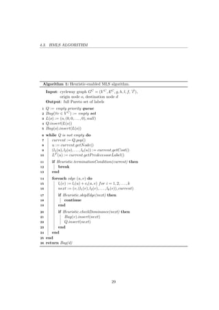
![4.4. HMLS ALGORITHM EVALUATION
minimum origin-destination distance is set to 500 m. The longest routes have ap-
proximately 4.5 km. We executed the MLS algorithm and the HMLS with all 15
heuristic combinations using the same generated 100 origin-destination pairs for each
graph Prague A, B, and C. Therefore, each heuristic combination is evaluated on
300 origin-destination pairs. Then we generated a total of 100 route requests for the
whole Prague graph where the origin-destination distance is set to be in the interval
from 500 to 10 000 m.
The parameters in the cost functions were set as follows. The average cruising
speed is s = 14 km/h, the penalty coefficient for uphill is al = 13 (according to the
route choice model developed in the user study [14]), the maximum downhill speed
multiplier is sdmax = 2.5, and the critical grade value is d c = 0.1.
Configuration parameters for the heuristics were optimised so as to maximise the
ratio between the algorithm runtime and the quality of the solution (see the next
section), as measured on the three graphs Prague A, B, and C. Specifically, the
following values were chosen: a
b = 1.25 for ellipse pruning, α = 1.6 for ratio-based
pruning, γ = c1
5 for cost-based pruning (c1 corresponds to a criteria value of the first
criterion), = 0.05 for -dominance, and (15, 2500, 4) for buckets (the triple defines
the buckets sizes for the three used criteria).
The results obtained in the experimental evaluation section are based on running
the algorithm on a single core of a 2.4 GHz Intel Xeon E5-2665 processor of a Linux
server. The source code of the HMLS algorithm and speedups for the multi-criteria
bicycle routing is openly available in a repository2 under LGPL license3.
4.4.2 Evaluation Metrics
We consider two categories of evaluation metrics: speed and quality. We use the
following to measure the algorithm speed:
• Average runtime in milliseconds for each origin-destination pair together with
its standard deviation σruntime.
• Average speedup over the standard, optimal MLS algorithm in terms of algo-
rithm runtime.
For a multi-criteria optimisation problem, solution quality cannot be simply defined
in terms of closeness to an optimal solution – instead, we define solution quality in
set terms as the closeness to the full Pareto set. To our best knowledge, there is not
a universal way to evaluate the quality of multi-criteria solutions. Therefore, we use
the following metrics to measure the quality of returned routes in the multi-criteria
bicycle routing problem:
• Average distance dc(Π∗, Π) of the heuristic Pareto set Π from the optimal Pareto
set Π∗ in the cost space. Distance dc(π∗, π) between two routes π∗ and π is mea-
sured as the Euclidean distance in the unit three-dimensional space of criteria
2
https://github.com/agents4its/cycleplanner/tree/mcspeedups
3
http://www.gnu.org/licenses/lgpl.html
33](https://image.slidesharecdn.com/5227de32-e56f-4573-b73a-9a28ea360750-170109080048/85/dissertation_hrncir_2016_final-41-320.jpg)
![4.4. HMLS ALGORITHM EVALUATION
values normalised to the [0, 1] range (min and max values of each criterion are
calculated for all plans in the optimal Pareto set Π∗ and the heuristic Pareto
set Π; the min value is mapped to 0 and the max to 1).
dc(Π∗
, Π) :=
1
|Π∗|
π∗∈Π∗
min
π∈Π
dc(π∗
, π)
Intuitively, dc(π∗, π) = 0.1 corresponds to a 6% optimality loss in each crite-
rion, assuming the difference to optimum is distributed equally across all three
criteria.
• Average distance dJ (Π∗, Π) of the heuristic Pareto set Π from the optimal Pareto
set Π∗ in the physical space. Jaccard distance dJ (π∗, π) [74] is used to measure
the dissimilarity between Pareto routes. For routes π∗ and π, i.e., sequences
of edges, the physical distance is computed by dividing the difference of the
sizes of the union and the intersection of the two route sets by the size of their
union. Reasonably, the physical distance definition for routes obeys the triangle
inequality.
dJ (π∗
, π) :=
| (π∗ ∪ π) | − | (π∗ ∩ π) |
| (π∗ ∪ π) |
dJ (Π∗
, Π) :=
1
|Π∗|
π∗∈Π∗
min
π∈Π
dJ (π∗
, π)
• Average number of routes |Π| in the Pareto set Π together with its standard
deviation σ|Π|.
• The percentage of Pareto routes Π% in heuristic Pareto set Π that are equal to
routes in the optimal Pareto set Π∗. For instance, if there are 10 routes in the
heuristic Pareto set Π and 6 routes are optimal, the percentage Π% = 60%.
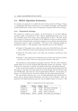
4.4.3 Results for Graphs Prague A, B, and C
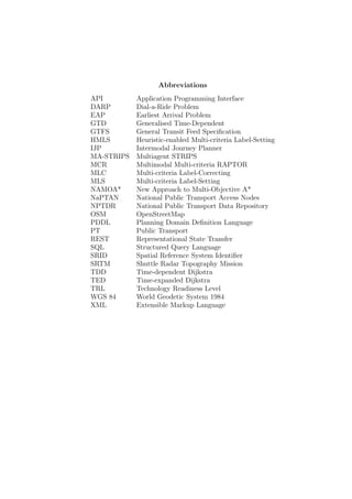
Table 4.2 summarises the evaluation of the HMLS algorithm and its heuristics us-
ing the neighbourhood-scale graphs Prague A, B, and C. The MLS algorithm is
used as a baseline for the evaluation of the proposed heuristics and their combina-
tions. Columns dc, dJ , and Π% are calculated with respect to the optimal Pareto
set Π∗ returned by the MLS algorithm. The MLS algorithm returns optimal solu-
tions (1647 routes in the Pareto set on average) at the expense of a prohibitively high
runtime.
As anticipated, all heuristic methods are significantly faster than the MLS algo-
rithm. First, we have compared the 15 evaluated methods using the following metrics:
the average runtime (from the speed category) and the average distance dc(Π∗, Π) in
the cost space (from the quality category). From the perspective of these two met-
rics, there are nine non-dominated combinations of heuristics, cf. filled-in bars in
34](https://image.slidesharecdn.com/5227de32-e56f-4573-b73a-9a28ea360750-170109080048/85/dissertation_hrncir_2016_final-42-320.jpg)
![4.4. HMLS ALGORITHM EVALUATION
Table4.2:EvaluationoftheheuristicperformanceonthreegraphsPragueA,B,andC.Primaryspeedandqualitymetrics
aremarkedbyboldcolumnheadings.Non-dominatedheuristiccombinationswithrespecttoprimaryspeedandquality
metricsaredenotedbyboldfont.
HeuristicSpeedupRuntime[ms]σruntime|Π|σ|Π|dcdJΠ%
MLS-898101110309716472390--100.00
HMLS+Buckets5851536129640440.1380.32355.25
HMLS+Cost1296946542193630.1780.33354.66
HMLS+Epsilon4490200131970.1950.42054.61
HMLS+Ratio3294458538357117316900.0540.07699.89
HMLS+Ratio+Buckets141563581835370.1730.34758.81
HMLS+Ratio+Cost2843161304480510.2110.36358.41
HMLS+Ratio+Epsilon730212398850.2330.44956.32
HMLS+Ellipse2434170956062163723900.0050.00899.98
HMLS+Ellipse+Buckets180149985340440.1420.32755.27
HMLS+Ellipse+Cost2933069389793630.1790.33454.79
HMLS+Ellipse+Epsilon965793104970.1990.42354.64
HMLS+Ellipse+Ratio4241675598290117116910.0560.08099.86
HMLS+Ellipse+Ratio+Buckets218341171535370.1750.34958.77
HMLS+Ellipse+Ratio+Cost4272103283080510.2110.36358.52
HMLS+Ellipse+Ratio+Epsilon110878184850.2320.44856.27
35](https://image.slidesharecdn.com/5227de32-e56f-4573-b73a-9a28ea360750-170109080048/85/dissertation_hrncir_2016_final-43-320.jpg)
![4.4. HMLS ALGORITHM EVALUATION
1
10
100
1 000
10 000
100 000
1 000 000
0.00
0.03
0.06
0.09
0.12
0.15
0.18
0.21
0.24
MLS
HMLS+Ellipse
HMLS+Ratio
HMLS+Ellipse+Ratio
HMLS+Buckets
HMLS+Ellipse+Buckets
HMLS+Ratio+Buckets
HMLS+Ellipse+Ratio+Buckets
HMLS+Cost
HMLS+Ellipse+Cost
HMLS+Epsilon
HMLS+Ellipse+Epsilon
HMLS+Ratio+Cost
HMLS+Ellipse+Ratio+Cost
HMLS+Ratio+Epsilon
HMLS+Ellipse+Ratio+Epsilon
runtime[ms]
distancedcincostspace
Average distance in cost space from the optimal Pareto set
Average runtime [ms]
Figure 4.5: Speed and quality for the HMLS algorithm and all heuristic combinations
sorted by the quality from the best (MLS on the left hand side) to the worst. Non-
dominated heuristic combinations have grey filled-in bars.
37](https://image.slidesharecdn.com/5227de32-e56f-4573-b73a-9a28ea360750-170109080048/85/dissertation_hrncir_2016_final-45-320.jpg)
![4.4. HMLS ALGORITHM EVALUATION
1
10
100
1000
0 1000 2000 3000 4000
runtime[ms]
direct origin-destination distance [m]
Figure 4.6: The runtime of HMLS+Ellipse+Epsilon in milliseconds in dependency on
the direct origin-destination distance.
0
2000
4000
6000
8000
10000
12000
0 1000 2000 3000 4000
Numberofroutesinthe
optimalParetoset
Direct origin-destination distance [m]
Figure 4.7: The number of routes in the optimal Pareto set |Π∗| in dependency on
the direct origin-destination distance.
|Π∗| in dependency on the direct origin-destination distance is shown in Figure 4.7.
The Pareto set can get very large. Therefore, a route selection method needs to
be implemented. It is an independent step for which various methods can be used.
In fact, we have already proposed a method based on clustering [103]. Regardless of
the selection method, the quality of the unfiltered results is essential as high-quality
solutions can be selected only if they are included in the unfiltered results set.
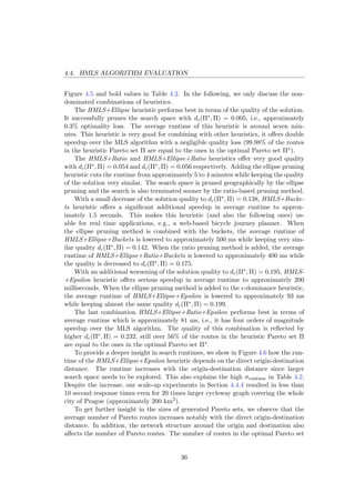
Finally, we have chosen a hilly area in Zizkov to illustrate the Pareto set of routes
in the physical space. In Figure 4.8, we illustrate the route distribution of the Pareto
sets returned by the MLS and HMLS algorithm with three different heuristic com-
binations. Each subfigure is provided with the name of the heuristic combination,
the size of the Pareto set (ranges from 532 to 6 routes) and the algorithm runtime
(ranges from 90 seconds to 372 ms). The more routes use a given cycleway network
segment, the wider is the depicted line. It can be observed that the heuristics return
a Pareto set of routes that very well corresponds to the optimal Pareto set.
38](https://image.slidesharecdn.com/5227de32-e56f-4573-b73a-9a28ea360750-170109080048/85/dissertation_hrncir_2016_final-46-320.jpg)
![4.4. HMLS ALGORITHM EVALUATION
To summarise, we have evaluated 15 different combinations of heuristics from
which 9 combinations dominated the others in terms of quality and speed. The
heuristics offer significant one to four orders of magnitude speedup over the MLS
algorithm in terms of average runtime. The speedup is achieved by lowering the
number of iterations and also the number of dominance checks in each iteration.
HMLS+Ellipse is the best heuristic in terms of quality of the produced Pareto set
while HMLS+Ellipse+Ratio+Epsilon is the best heuristic in terms of average run-
time. Taking into the account the trade-off between the quality of a solution and
the provided speedup, we consider HMLS+Ellipse+Epsilon heuristic to have the best
ratio between the quality and speed.
4.4.4 Scale-up Results for the Whole Prague Graph
In order to show the scalability of the proposed heuristics to city-scale routing, we
evaluate the heuristics on the graph of the whole Prague city which is approximately
20 times bigger than each of the graphs Prague A, B, and C. The results are sum-
marised in Table 4.3. We present only a subset of statistics (compared to Table 4.2)
since the graph is too large to get an optimal Pareto set by the MLS algorithm. We
show the total number of requests finished in the imposed 15-minutes limit, average
runtime in milliseconds, and average size of the Pareto set.
We have evaluated all combinations of heuristics; they offer average runtimes be-
tween 5 and 260 seconds. Eight evaluated heuristic combinations successfully return
Table 4.3: Evaluation of the heuristic performance on the whole Prague graph.
Heuristic 15 min Runtime [ms] σruntime |Π|
HMLS+Buckets 0 - - -
HMLS+Cost 100 70 734 25 311 72
HMLS+Epsilon 100 15 759 4 859 12
HMLS+Ratio 14 168 302 250 902 402
HMLS+Ratio+Buckets 51 176 810 225 504 126
HMLS+Ratio+Cost 100 49 948 29 421 69
HMLS+Ratio+Epsilon 100 8 847 6 512 11
HMLS+Ellipse 18 260 278 313 214 918
HMLS+Ellipse+Buckets 72 128 096 194 328 244
HMLS+Ellipse+Cost 100 33 474 25 008 72
HMLS+Ellipse+Epsilon 100 5 306 5 667 11
HMLS+Ellipse+Ratio 20 112 333 159 589 768
HMLS+Ellipse+Ratio+Buckets 76 130 738 206 001 242
HMLS+Ellipse+Ratio+Cost 100 32 799 25 235 69
HMLS+Ellipse+Ratio+Epsilon 100 4 834 5 159 11
NAMOA*+TC 100 106 436 192 884 2 984
40](https://image.slidesharecdn.com/5227de32-e56f-4573-b73a-9a28ea360750-170109080048/85/dissertation_hrncir_2016_final-48-320.jpg)
![4.5. VALIDATION IN REAL-WORLD DEPLOYMENTS
solutions for all 100 origin-destination pairs in the 15-minutes time limit. We can
observe the behaviour of the ellipse pruning heuristic that does not significantly de-
crease the size of the Pareto set yet offers solid speedup consistent with the results on
the graphs Prague A, B, and C. The best performing combinations of heuristics are
HMLS+Ellipse+Epsilon and HMLS+Ellipse+Ratio+Epsilon with practically usable
average runtime of 5 seconds. This result is consistent with our evaluation of the
heuristics on the graphs Prague A, B, C where the two heuristics also performs best
in terms of average runtime.
Finally, we compared the HMLS algorithm with heuristic speedups to the opti-
mal NAMOA* algorithm [76] with the Tung & Chew (TC) heuristic [111]. The TC
heuristic works as a preprocessing step where for each criterion a backward Dijkstra’s
algorithm is executed from the destination to all nodes in the graph. The prepro-
cessing calculates the values of a perfect heuristic function, i.e., true cost values from
each node to the destination, for the NAMOA* algorithm. Using the whole Prague
graph, the preprocessing takes 444 ms on average. The NAMOA* algorithm with the
TC heuristic successfully returned solutions for all 100 origin-destination pairs; the
total runtime of the algorithm was 106 seconds on average. On the runtime side, the
algorithm is better than 6 combinations of heuristics. However the best performing
heuristic combination HMLS+Ellipse+Epsilon is 50 times faster than the NAMOA*
algorithm with TC heuristic. On the quality side, the algorithm outperformed HMLS
algorithm with each heuristic combination since it delivered optimal Pareto sets of
routes (2 984 on average). Altogether, for the problems where there is not neces-
sary to deliver the whole Pareto set of solutions (e.g., multi-criteria bicycle routing
problem) the HMLS+Ellipse+Epsilon and HMLS+Ellipse+Ratio+Epsilon deliver 50
times better runtime than the NAMOA* algorithm with TC heuristic.
To summarise, we are able to solve multi-criteria bicycle routing problem on
the large graph instance with tens of thousands of nodes and edges while achieving
practically usable runtimes of 5 seconds.
4.5 Validation in Real-World Deployments
To fulfil Research objective 3, we have performed validation using real-world de-
ployments. We think that deploying our approach in the operational environment
(TRL 74) is the way to find out the issues that needs to be solved to use the ap-
proach in practise. These important issues cannot be found at the stage of algorithm
design/evaluation. Furthermore, it is a way to discover open research questions and
next research steps. This is a place where two disciplines – research and engineering –
meets. Based on real-world deployments, we have acquired useful experience which is
common with other problems solved in this thesis so we have concentrated the lessons
learned in Chapter 7. In the remaining part of this section, we describe details that
are specific for the deployment of bicycle routing system.
4
http://ec.europa.eu/research/participants/data/ref/h2020/wp/2014_2015/annexes/
h2020-wp1415-annex-g-trl_en.pdf
41](https://image.slidesharecdn.com/5227de32-e56f-4573-b73a-9a28ea360750-170109080048/85/dissertation_hrncir_2016_final-49-320.jpg)
![4.5. VALIDATION IN REAL-WORLD DEPLOYMENTS
Bicycle Routing System Backend
Bicycle Routing Core
RESTful API
Android App
Web App
Data Importer
OSM XML
Data
MongoDB
Storage
Figure 4.9: Architecture of the bicycle routing system.
Figure 4.10: Android App frontend for the bicycle routing system allows finding
bicycle routes, navigate to a destination, and track journeys (developed by Jan Linka).
To begin with, we have deployed a simplified version of the bicycle routing algo-
rithm as a bicycle routing system with an open RESTful API. Architecture of the
system is presented in Figure 4.9. The system consists of two main parts. The first
part is the bicycle routing system backend that is primarily responsible for finding
the Pareto set of routes based on the origin-destination pairs. At the backend, Data
Importer builds the cycleway graphs from OSM XML files. The graphs are then
used by the Bicycle Routing Core component that performs the routing. Finally, the
communication with the backend is managed through the open RESTful API that
uses a NoSQL MongoDB database to store found routes, feedback from cyclists, and
tracked bicycle journeys. An efficient implementation of the bicycle routing system
backend has been carried out by Pavol ˇZileck´y in his master thesis (supervised by the
author of the thesis) [118]. More details about backend internal workings and about
42](https://image.slidesharecdn.com/5227de32-e56f-4573-b73a-9a28ea360750-170109080048/85/dissertation_hrncir_2016_final-50-320.jpg)
![4.5. VALIDATION IN REAL-WORLD DEPLOYMENTS
Figure 4.11: Smartphone with our app mounted on bicycle handlebars helps users
with the navigation in cities which is often challenging due to fragmented cycling
infrastructure.
Figure 4.12: Tracked GPS points in the centre of Prague.
the API can be found in his thesis.
The second part of the system is composed from the Android App and Web App
frontends. On the one hand, the Android App has been developed by Jan Linka
in his bachelor thesis (supervised by the author of the thesis) [75] with a valuable
43](https://image.slidesharecdn.com/5227de32-e56f-4573-b73a-9a28ea360750-170109080048/85/dissertation_hrncir_2016_final-51-320.jpg)
![4.6. CONTRIBUTIONS AND SUMMARY
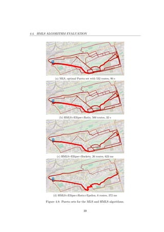
the competition. The tracked data are depicted in Figure 4.12. The GPS tracked data
has been mapped to the cycling network by Daniel Sluneˇcko in his bachelor thesis
(supervised by the author of the thesis) [102] and then a map of cycling traffic intensity
and cycling speed has been created by Filip Langr, see Figure 4.13. Importantly, we
plan to incorporate the tracked journeys into the routing process (see Section 8.1) to
improve the quality of route suggestions. Furthermore, the tracked journeys can be
used by the municipality to improve the quality of the infrastructure for cyclists such
as adding new cycle lanes in streets that are frequently used by the cyclists. On the
other hand, the Web App has been developed by Tom´aˇs Fiˇser and is freely available6.
It is able to show the found set of routes and also their quality in terms of criteria,
cf. Figure 4.14.
4.6 Contributions and Summary
In this chapter, we have investigated a multi-criteria approach to urban bicycle rout-
ing. Our contributions with respect to state-of-the-art techniques described in Sec-
tion 2.2 are summarised as follows.
In contrast to existing work, we have provided a well-grounded formal model of
multi-criteria bicycle routing and have applied a novel heuristic-enabled multi-criteria
shortest path algorithm to find a diverse set of cycling routes. As a result, we have
made bicycle routing that properly considers multiple realistic route choice criteria
fast enough for practical, interactive use. Our method produces routes closely ap-
proximating the full Pareto set in hundreds of milliseconds when routing on a neigh-
bourhood scale and in seconds when routing on a city-wide scale. Further speedups
are possible through low-level optimisation of data structures and the algorithmic
logic.
We have achieved these results by employing five heuristic speedup techniques for
multi-criteria shortest path search. The speedup heuristics provide a variable trade-
off between the search time and the completeness and quality of the suggested routes
and they enable fast response times without severely compromising the quality of the
results. Although the heuristics are relatively simple, their application in the context
of bicycle routing is novel and their effect is very significant. Because real-world
speedup performance may differ significantly from the performance on general multi-
criteria shortest path problems, our work is important for properly understanding
realistic performance trade-offs in developing efficient bicycle routing algorithms.
We have evaluated our approach extensively in the challenging conditions of the
city of Prague, which features complex geography and fragmented cycling infrastruc-
ture. The evaluation has confirmed the usefulness of the multi-criteria approach to
bicycle routing. To conclude, the bicycle routing system has been validated in real-
world deployments via a RESTful API used by Android App and Web App frontends.
The system has been discussed with the experts on cycling from Auto*Mat NGO and
has been used by hundreds of cyclists in the Bike2Work competition in May 2015.
6
http://its.felk.cvut.cz/cycleplanner2/
45](https://image.slidesharecdn.com/5227de32-e56f-4573-b73a-9a28ea360750-170109080048/85/dissertation_hrncir_2016_final-53-320.jpg)
![4.6. CONTRIBUTIONS AND SUMMARY
The multi-criteria bicycle routing algorithm has been devised in collaboration
with Pavol ˇZileck´y and Qing Song. Pavol has efficiently implemented the HMLS
algorithm including speedups and executed the experiments. He has also created
a simple visualisation tool used in Figure 4.8 and contributed to the description of the
HMLS algorithm in Section 4.3 and pseudocodes of speedups in Appendix B. Qing has
contributed to related work regarding multi-criteria bicycle routing in Section 2.2 and
definition of the bicycle routing problem in Section 4.1.1. She has also collaborated
on the design of ratio-based pruning and cost-based pruning heuristics. Finally, this
topic is covered by the following articles [66, 67, 68, 103].
46](https://image.slidesharecdn.com/5227de32-e56f-4573-b73a-9a28ea360750-170109080048/85/dissertation_hrncir_2016_final-54-320.jpg)
![Chapter 5
Intermodal Journey Planning
The advent of new types of mobility services, such as bike, scooter, and car sharing,
real-time carpooling or next-generation taxi, has further expanded the already rich
portfolio of mobility means available in modern cities. Providing intelligent tools that
would help citizens make the best use of mobility services on offer is thus needed more
than ever [92]. Despite recent algorithmic advances [5], existing planners available
in practise, such as Google Maps1 or Here.com2, address this need only partially. In
particular, they only consider a limited subset of transport modes and their combina-
tions, and they only provide limited ways for users to express their travel preferences.
Based on the motivation above, we progress to study the single-agent single-
criteria intermodal routing problem. The problem is most often formalised as the ear-
liest arrival problem (EAP), i.e., the problem of finding the earliest arrival at a desti-
nation given a departure date and time from an origin. The earliest arrival problem
has been widely studied and numerous algorithms and speedup techniques exist for
solving it on road network graphs and networks of public transport (PT) services.
Until recently, little work has been done on solving the earliest arrival problem for
journey plans allowing general combinations of individual and public transport modes,
the work of Horn [60], and Yu and Lu [117] being notable exceptions. However, in
parallel to our research, several approaches aiming to solve the intermodal routing
problem have emerged (Delling et al. [27], Gundling et al. [54], and Kirchler [73]).
This means that this problem has become topical.
In our work, we focus on solving the intermodal variant of the EAP. We use the
term intermodal in order to stress that we consider modes and combinations thereof
that go beyond what is supported in existing multimodal journey planners. Our main
contribution with respect to state-of-the-art techniques described in Section 2.4 lies
in a representation-centric approach to solving the intermodal EAP. Thus, instead of
providing complex, purpose-specific journey planning algorithms, we have introduced
a generalised time-dependent graph (see Section 3.2.2) that allows representing the
intermodal EAP as a standard graph search problem and consequently use general
1
http://maps.google.com
2
http://here.com
47](https://image.slidesharecdn.com/5227de32-e56f-4573-b73a-9a28ea360750-170109080048/85/dissertation_hrncir_2016_final-55-320.jpg)
![5.1. INTERMODAL EARLIEST ARRIVAL PROBLEM
shortest path algorithms to solve it. What is more, studying this approach further on
lead to related work on PT network analysis [84, 85] and on integration of multiple
journey planners [83].
We treat the problem in a deterministic setting assuming no uncertainty in any of
the attributes of the planning graph. In addition to the generalised time-dependent
graph representation, we also introduce the concept of journey plan templates. Jour-
ney plan templates provide a powerful way of parameterising the operation of the
planner and allow the user or the administrator of the journey planner to obtain
plans that best meet their constraints and preferences. Furthermore, the templates
constrain the search space and therefore speed up journey planning.
5.1 Intermodal Earliest Arrival Problem
In this section, we provide the formalisation of the intermodal earliest arrival problem.
The intermodal journey planner (IJP) should be able to plan journeys which use any
combination of a full range of transport modes, including scheduled PT (e.g., bus,
underground, tram, train, ferry), individual transport (e.g., walk, bike, shared bike
and car), and on-demand transport (e.g., taxi). The term intermodal emphasises
the fact that the planner should be able to plan a journey using a combination of
a full range of transport modes, as compared to existing planners that are only able
to handle a subset of transport modes and their combinations (e.g., a cycle planner,
a scheduled PT planner).
Our approach to solving the intermodal EAP relies on the newly proposed gen-
eralised time-dependent (GTD) graph defined in Section 3.2.2, which allows repre-
senting the combined road network (for individual and on-demand modes) and PT
network (for PT modes) in a single structure. Below, we first describe the notions
of a journey leg and a journey plan. Then, we define two variants of the intermodal
earliest arrival problem.
5.1.1 Journey Leg and Journey Plan
Let the journey leg be a part of a journey plan that is either covered by the traveller
on foot or by a movement by one and only one vehicle from one location to another.
Formally, the journey leg L = ((v1, w1), . . . , (vk, wk)) is defined as a sequence of
|L| = k edges (vj, wj) ∈ E. Edges are a finer-grained decomposition of a journey leg
and represent the lowest-level, atomic parts of any journey plan. Then the journey
plan is a quadruple π = (P, σ, φ, ψ):
• P = (L1, . . . , Ln) is a sequence of |P| = n journey legs Li.
• Function σ denotes the mode of transport σ(Li) ∈ M that is used for journey
leg Li.
• Function φ : E → N returns the departure time from v for each edge (v, w) ∈ E.
48](https://image.slidesharecdn.com/5227de32-e56f-4573-b73a-9a28ea360750-170109080048/85/dissertation_hrncir_2016_final-56-320.jpg)
![5.1. INTERMODAL EARLIEST ARRIVAL PROBLEM
• Function ψ : E → N returns the arrival time at w for each edge (v, w) ∈ E.
Let L[j] be the j-th element of a sequence of elements L and |L| be the number of
elements in L. Let ξ(P) be the flattened plan constructed as the concatenation of all
edges in all journey legs Li ∈ P:
ξ(P) = (L1[1], . . . , L1[|L1|], . . . , Ln[1], . . . , Ln[|Ln|])
5.1.2 Intermodal Earliest Arrival Problem
The intermodal earliest arrival problem is a pair J = (G, r), where:
• G = (V, E, ρ, µ, χ) is a GTD graph
• r = (o, d, t) is a journey request specifying an origin o ∈ V , a destination d ∈ V ,
and a time of departure t ∈ N
A journey plan π = (P, σ, φ, ψ), where P = (L1, . . . , Ln), is then a solution of the
intermodal earliest arrival problem J = (G, r) if and only if all the following conditions
hold:
1. Journey plan starts at the origin:
o = v where (v, w) = L1[1]
2. Journey plan ends at the destination:
d = w where (v, w) = Ln[|Ln|]
3. All edges are present in the GTD graph:
∀(v, w) ∈ ξ(P) : (v, w) ∈ E
4. Edges form a path in the GTD graph:
∀j ∈ {1, . . . , |ξ(P)| − 1} :
(v, w) = ξ(P)[j] ∧ (w, x) = ξ(P)[j + 1]
5.1.3 Intermodal EAP with Templates
For the intermodal earliest arrival problem with templates, we introduce the notion
of a journey plan template. As mentioned in the introduction, journey plan templates
give users and journey planner administrators a powerful way of parameterising the
journey planner to obtain plans that best meet their constraints and preferences.
For instance, a journey plan template that prefers environmentally friendly modes of
transport can be designed by a journey planner administrator (e.g., a combination of
walk and shared bike).
A journey plan template constrain the journey plan in the permitted combination
of modes on the level of journey legs. A journey plan template τ is defined as a regular
expression over the transport modes alphabet M. As an example, we list three
templates3:
3
POSIX Extended Regular Expression syntax is used.
49](https://image.slidesharecdn.com/5227de32-e56f-4573-b73a-9a28ea360750-170109080048/85/dissertation_hrncir_2016_final-57-320.jpg)
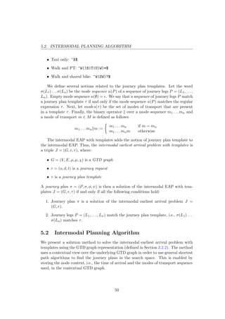
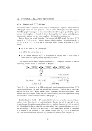
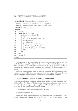
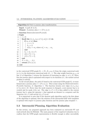
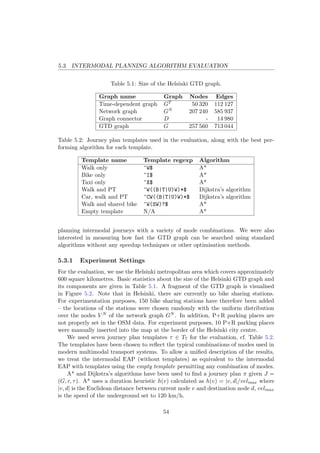
![5.3. INTERMODAL PLANNING ALGORITHM EVALUATION
walk only bike and walk PT roads
Figure 5.2: Visualisation of a 2.4 km by 2.4 km fragment of the Helsinki GTD graph.
Edge colours denote the modes of transport permitted at each edge, cf. legend. All
other combinations of modes (e.g., car and taxi, bike only) are marked red. There
are approximately 9 500 nodes and 27 700 edges in the visualisation.
Following initial experiments, the better algorithm of the two has been chosen
for each template τ ∈ T7. The templates τ ∈ T7 and their corresponding chosen
algorithms are listed in Table 5.2. Consequently, all templates use A* except the
walk and PT template and car, walk and PT template where the Euclidean distance
heuristic slows-down the A* search process [52] so the Dijkstra’s algorithm is used.
The set of instances of the intermodal EAP with templates Q for the experiment
were created in the following way. First, n = 10 000 origin-destination-departure
triples Qt = ((o1, d1, t1), . . . , (on, dn, tn)) were sampled using the uniform distribution
over the coordinates of Helsinki area and the uniform distribution over the time
interval from 8:00 to 18:00 on 17 Jan 2013. The maximum origin-destination distance
was set to 40 km to exclude long trips that are not usual in the urban setting.
Then the origin and destination coordinates were converted to origin and desti-
nation nodes from graph G. Let δ(c, m) be a function that returns the nearest node
in the GTD graph G given a coordinate c and a mode of transport m. For example,
for the walk mode, the nearest node on a pavement is returned. Then the set of
|Q| = 70 000 instances of the intermodal EAP with templates is constructed. Each
of the origin-destination-departure triples Qt is combined with all journey templates
55](https://image.slidesharecdn.com/5227de32-e56f-4573-b73a-9a28ea360750-170109080048/85/dissertation_hrncir_2016_final-63-320.jpg)
![5.3. INTERMODAL PLANNING ALGORITHM EVALUATION
0
100
200
300
400
500
600
0 10 20 30 40
runtime[ms]
origin-destination distance [km]
Figure 5.3: Runtime against origin-destination distance (taxi only template, 1 000
randomly selected requests).
0
250
500
750
1000
1250
0 10 20 30 40
runtime[ms]
origin-destination distance [km]
Figure 5.4: Runtime against origin-destination distance (walk and PT template, 1000
randomly selected requests).
Figures 5.3 and 5.4 show scatter plots of the search runtime versus the origin-
destination distance for 1 000 randomly selected requests. It can be observed that
runtimes for the taxi only template in Figure 5.3 are more strongly correlated on
the origin-destination distance than the runtimes of the walk and PT template in
Figure 5.4.
57](https://image.slidesharecdn.com/5227de32-e56f-4573-b73a-9a28ea360750-170109080048/85/dissertation_hrncir_2016_final-65-320.jpg)
![5.4. VALIDATION IN REAL-WORLD DEPLOYMENTS
Intermodal Journey Planning System Backend
RESTful API
Android App
Web App
Data Importer and Validator
PostgreSQL
Storage
MongoDB
Storage
Intermodal
Planning Core
Journey Plan
Recommender
Mobility
Resource
Negotiator
Figure 5.5: Architecture of the intermodal journey planning system.
(2) the business logic layer implementing the journey planning functionality, and
(3) the API layer providing the backend functionality to the frontends. The second
part of the system is composed from the Android App and Web App frontends. See
Figure 5.5 for the overview of the architecture. Individual backend components are
described below in more details.
Data Importer and Validator: This component was created in collaboration with
Zdenˇek Moler, Radek Hol´y, and Daniel Stahr and is responsible for creating the GTD
graph (defined in Section 3.2.2) that is then used by the Intermodal Planning Core
component. The network graph (roads, cycleways, and pavements) is loaded from
the XML OSM file. The time-dependent graph for the PT network is loaded from
a PostgreSQL database with a GTFS schema. The planner uses a range of additional
data, including the information about vehicle and bicycle sharing stations and parking
facilities. Upon import, information from different data sources is translated, cross-
referenced and integrated into the GTD graph. Resulting GTD graph for Milan is
shown in Figure 5.6. This component is also responsible for data validation, e.g., to
check whether the timetables do not contain connections with zero runtimes.
Intermodal Planning Core: This component uses intermodal planning algorithm
described in Section 5.2 and is responsible for planning multi-leg journeys utilizing
the full range of transport modes. To promote modularity and extensibility, the
planner employs a novel multi-critics architecture that relies on the notion of critics,
specialised modules for evaluating candidate journey plans from a certain perspec-
tive, e.g., price, emissions or user convenience. The multi-critics architecture allows
introducing new concerns to journey planning without modifying the core planning
logic. At the moment, the planner evaluates duration, distance, price, CO2 emissions,
physical effort, and user satisfaction of each journey plan.
Journey Plan Recommender: This component developed by Codina et al. [17] is
responsible for making personalised trip recommendations best reflecting the user’s
59](https://image.slidesharecdn.com/5227de32-e56f-4573-b73a-9a28ea360750-170109080048/85/dissertation_hrncir_2016_final-67-320.jpg)
![5.4. VALIDATION IN REAL-WORLD DEPLOYMENTS
walk only bike and walk PT roads
Figure 5.6: GTD graph of Milan (221 707 nodes and 601 695 edges).
situation, needs and preferences. Technically, the recommender uses the latest devel-
opments in hybrid recommendation, combining content-based approaches and collab-
orative approaches. It forecasts user satisfaction with respect to given journey plans
and returns it to the intermodal planner core through the critic interface. In partic-
ular, user satisfaction with respect to journey plans and journey legs is expressed by
an Integer value ranging from 0 (definitely dislike) to 100 (definitely like).
Mobility Resource Negotiator: This component developed by Finnegan et al. [44]
interacts with the transport service providers on behalf of the user and allows price
calculation together with selecting and reserving services that best match the re-
quirements of the journey plan under consideration. Mobility resources required for
carrying out recommended journeys are allocated through a (semi-)automated nego-
tiation mechanisms using an open tendering process [108]. The component is inte-
grated with the intermodal planner core through the critic interface which provides
the planner with the feedback on the expected availability and price of requested
mobility resources (e.g., Helsinki Region Transport SMS public transport ticket and
taxi booking in Milan).
The backend part of the system is used via a RESTful API which allows additional,
third party applications and services to be developed on top of the planner. Currently,
there are three frontends using the API. To begin with, a Web App and Android App
60](https://image.slidesharecdn.com/5227de32-e56f-4573-b73a-9a28ea360750-170109080048/85/dissertation_hrncir_2016_final-68-320.jpg)
![5.4. VALIDATION IN REAL-WORLD DEPLOYMENTS
Figure 5.7: Simplified Web App frontend for the planner. A set of intermodal journey
plans returned by the planner for the city of Milan is shown together with the values
of six supported journey criteria for each plan (developed by Pavol ˇZileck´y).
developed by the superhub project is available as part of the full superhub software
platform [16]. Second, a simplified Web App frontend which allows users to submit
journey planning requests and interactively explore recommended journey plans has
been developed by Pavol ˇZileck´y. The Web App is depicted in Figure 5.7 and also
available online5.
We deployed the presented planner, along with additional components, as part of
the superhub project’s field trials in three large European cities (Barcelona, Helsinki,
and Milan). Several hundred trial participants used the planner for a period of six
weeks in autumn 2014. The feedback was largely positive – the users commended the
quality of plans and the responsiveness of the system, which was able to return plans
within one second in most circumstances.
5.4.1 Journey Planning Quality
Journey planning in a city represented by a graph with several hundred thousands
of nodes and edges, cf. Table 5.1, is a very complex task where it is impossible for
a human to find an optimal solution manually. This means that there is no other
possibility to check the quality of journey planning than to compare journey plans
with a different planner. To automate the comparison process, it is needed that the
5
http://transport.felk.cvut.cz/journeyplanner/
61](https://image.slidesharecdn.com/5227de32-e56f-4573-b73a-9a28ea360750-170109080048/85/dissertation_hrncir_2016_final-69-320.jpg)
![5.4. VALIDATION IN REAL-WORLD DEPLOYMENTS
Table 5.4: Results of intermodal planner comparison for individual modes (cities are
abbreviated to B = Barcelona, H = Helsinki, and M = Milan).
Duration Distance Intermodal planner
difference [%] difference [%] dominated plans [%]
Template B H M B H M B H M
Walk only -13.1 -5.9 -3.2 -8.1 -2.3 -0.8 82.0 91.9 87.0
Bike only N/A 4.4 N/A N/A -10.5 N/A N/A 39.1 N/A
Car only -20.0 -17.3 -35.4 -14.1 -3.9 -9.1 85.9 86.8 99.0
second planner has an open API that can be queried automatically. As the second
planner, we chose Google Directions API6 that uses state-of-the-art journey planning
technology (also used in Google Maps) and provides an open API.
We compared the quality of the intermodal planner (that uses intermodal planning
algorithm defined in Section 5.2) for the following four journey plan templates that are
also supported by Google Directions API: “Walk only”, “Bike only”, “Car only”, and
“Walk and PT”. For each city, we created 100 random origin-destination-departure
triples that were used for the comparison. The results of the comparison for individual
templates “Walk only”, “Bike only”, and “Car only” are shown in Table 5.4. The
results of the comparison for “Walk and PT” template are shown in Table 5.5. In
both tables holds that when the duration/distance/number of transfers difference in
% is smaller than zero, it means that intermodal planner have found journey plans
with lower duration/distance/number of transfers (the difference is calculated over
the 100 random queries).
In this paragraph, we discuss the results of individual journey plan templates
shown in Table 5.4. Intermodal planner dominated plans column provides a percent-
age of plans that have strictly better duration than plans found by Google Directions
API. It is important to say that the differences is partially caused by a fact that
intermodal planner uses OSM maps whereas Google Directions API uses their own
maps. Regarding walk, the intermodal planner is slightly better in all three cities
(we use the same 5 km/h walking speed as Google does). Bike journey planning was
tested only in Helsinki since Google Directions API did not support it in Barcelona
and Milan (denoted by N/A in the table). Intermodal planner provides bike jour-
ney plans with similar duration and slightly lower distance than Google Directions
API. With the car, intermodal planner finds plans with slightly shorter distance than
Google Directions API. However, intermodal planner is underestimating the duration
of car journey plans.
In the following paragraphs, we discuss the results of “Walk and PT” template
shown in Table 5.5. Both planners return multiple “Walk and PT” plans, we than
compare the ones that have the minimum number of transfers.
Regarding plan duration, the intermodal planner finds slightly shorter plans in
Barcelona and Helsinki. In Milan, the duration difference is much larger (-29.1%).
6
https://developers.google.com/maps/documentation/directions/
62](https://image.slidesharecdn.com/5227de32-e56f-4573-b73a-9a28ea360750-170109080048/85/dissertation_hrncir_2016_final-70-320.jpg)
![5.5. CONTRIBUTIONS AND SUMMARY
Table 5.5: Results of intermodal planner comparison for “Walk and PT” template.
Barcelona Helsinki Milan
Duration difference [%] -7.1 -2.4 -29.1
Number of transfers difference [%] -15.4 20.0 75.0
Walk distance difference [%] 32.3 24.1 -55.4
Intermodal planner dominated plans [%] 70.7 37.9 44.2
Google planner dominated plans [%] 22.0 43.2 18.6
Non-dominated plans [%] 7.3 18.9 37.2
The difference is caused by different GTFS data used by the two planners. Intermodal
planner is missing Trenord trains7 whereas Google planner is missing ATM operator8
that have quite a large transport network (i.e., Google then finds walk journey plans
instead of using, e.g., underground from the ATM transport network).
Regarding the number of transfers, the intermodal planner is better in Barcelona
but provides plans with more transfers in Helsinki. In Milan, the high difference
(75%) is caused by the missing ATM data in Google Directions API; the Google
planner uses often walk instead of scheduled PT services resulting in significantly
lower number of transfers.
Regarding walk distance, the intermodal planner is much better in Milan due to
the data issue mentioned above. In Barcelona and Helsinki, intermodal planner offers
plans with more walking than Google. This can be easily improved by tuning the
maximum walking distance parameter.
Finally, we discuss the quality of plans when two criteria – duration and number
of transfers – are taken into account. The intermodal planner dominated plans means
a percentage of plans that have strictly better duration and better or the same number
of transfers than plans found by Google Directions API. By this overall comparison,
we can observe that intermodal planner is better in Barcelona and Milan. In Helsinki,
both planners return plans with similar quality.
To summarize, despite having a broader set of features, the quality of journey
plans returned by the intermodal planner compares very well (in terms of journey
duration and number of transfers) with state-of-the-art commercial journey planners
that only support a limited number of transport modes and mode combinations.
5.5 Contributions and Summary
In this chapter, we have presented an advanced intermodal journey planner designed
to help travellers to take the full advantage of the increasingly richer and conse-
quently more complex offer of mobility services available in modern cities. Our main
contribution with respect to state-of-the-art techniques presented in Section 2.4 is
7
http://www.trenord.it/en/
8
http://www.atm.it/en/
63](https://image.slidesharecdn.com/5227de32-e56f-4573-b73a-9a28ea360750-170109080048/85/dissertation_hrncir_2016_final-71-320.jpg)
![5.5. CONTRIBUTIONS AND SUMMARY
a representation-centric approach to solving the intermodal journey planning prob-
lem. Thus, instead of providing complex, purpose-specific journey planning algo-
rithms, we have introduced a generalised time-dependent graph that allows repre-
senting the intermodal journey planning problem as a standard graph search problem
and consequently use general shortest path algorithms to solve it.
Experiments on realistic network data about the Helsinki transport system con-
firmed the viability of the approach – the planner was able to find a diverse set of
journey plans and achieve runtimes which, although noticeably higher compared to
algorithms optimised for basic variants of the earliest arrival problem, are generally
usable. Finally, the presented planner has been validated in real-world deployments
in an intermodal journey planning system with a RESTful API. The system has been
deployed along with additional components as part of the superhub project’s field
trials in three large European cities (Barcelona, Helsinki, and Milan). In 2014, sev-
eral hundreds of trial participants were using the planner through Android App and
Web App for a period of one month. The feedback was mostly positive – the users
commended the quality of plans and the responsiveness of the system, which was able
to return plans within one second in most circumstances.
The research presented in this chapter was published in the following articles [63,
71]. The research on this topic has led to related work on PT network analysis [84, 85]
and on the integration of multiple journey planners [83].
64](https://image.slidesharecdn.com/5227de32-e56f-4573-b73a-9a28ea360750-170109080048/85/dissertation_hrncir_2016_final-72-320.jpg)
![Chapter 6
Ridesharing on Timetabled
Transport Services
Lastly, travelling is an important and frequent activity, yet people willing to travel
have to face problems with rising fuel prices, carbon footprint, and traffic jams. One
way to tackle these problems is through ridesharing, i.e., purposeful and explicit
planning to create groups of people that travel together in a single vehicle for parts
of the journey. Participants in such schemes can benefit from ridesharing in several
ways: sharing parts of a journey may reduce cost (e.g., through group tickets), carbon
footprint (e.g., when sharing a private car), and travellers can enjoy the company of
others on a long journey. In more advanced scenarios one could even imagine this
being combined with working together or holding meetings while travelling.
Following the motivation above, we finally explore the field of multiagent single-
criteria multimodal routing, i.e., multimodal ridesharing. The potential of improving
travel sharing technology has great application value due to its ability to reduce the
environmental impact of travelling while providing benefits to travellers at the same
time. In general, ridesharing is a widely studied problem – existing work, however,
focuses exclusively on ridesharing using vehicles that can move freely on a road trans-
port network. This overlooks the potential for innovative future transport schemes
that might exploit ridesharing using timetabled public transport. Here, customised
group discount schemes could be devised to balance the load across different times of
the day, or to make more efficient use of the capacity of public modes of transport.
Also, joint travel can be used to increase the comfort and safety of individuals, e.g.,
for female travellers using night buses, or groups of schoolchildren. To the best of our
knowledge, no existing work seems to attempt to compute joint travel plans based on
public transport timetables and geographical stop locations, let alone in a way that
takes into account the strategic nature of the problem, which comes about through
the different (and potentially conflicting) preferences of individual travellers.
From the point of view of (multiagent) planning [24], i.e., the problem of synthesis-
ing sequences of actions to reach a certain goal – in this case, arrival at a destination
from a given point of departure – for several travellers in parallel, ridesharing on
65](https://image.slidesharecdn.com/5227de32-e56f-4573-b73a-9a28ea360750-170109080048/85/dissertation_hrncir_2016_final-73-320.jpg)
![6.1. TIMETABLED TRANSPORT RIDESHARING PROBLEM
timetabled services presents itself as a very complex application scenario: To begin
with, even if one restricted oneself to centralised planning, the domain is huge – public
transport data for the UK alone currently involves 240 590 timetable connections for
trains and coaches (even excluding local city buses), which would have to be trans-
lated to a quarter of a million planning actions, at least in a naive formalisation of
the domain. This is the case even if we assume a non-strategic setting, where indi-
viduals’ preferences are not taken into account, and we are simply looking for a set of
itinerary that gets everybody to their destination, without any regard for how costly
this might be for the individual, or how the joint plan might favour some agents while
putting others at a disadvantage. Moreover, considering a strategic setting where we
are looking for a plan for multiple self-interested agents that are willing to cooperate
only if it is beneficial for them is known to be exponentially harder than planning for
each agent individually [12]. Yet any automated service that proposes joint journeys
would have to guarantee such strategic properties in order to be acceptable for human
users.
We proposed a solution employing strategic multiagent planning that guaran-
tees that for any shared journey plan found, each individual is better off taking the
shared ride rather than travelling alone, thus providing a clear incentive to partici-
pate in it. The core of our algorithm is based on a domain-independent best-response
planning [72] approach which is a planner that can solve strategic multiagent plan-
ning problems of the scale required, and whose properties and assumptions combine
particularly well with the ridesharing problem in hand.
6.1 Timetabled Transport Ridesharing Problem
Informally, the problem we are trying to solve is the following: Assume a (potentially
very large) set of agents who represent individual travellers, with their individual trips
specified in terms of origin and target location. Assume also that the agents want to
optimise the individual utility accrued from a trip, and this utility may depend on the
travel cost and number of people travelling along each leg of the journey (generally,
we will assume that group travel has a positive effect on utility, as we want to study
the impact of this very aspect on travel behaviour). Based on this information, we
are looking for an algorithm that can identify appropriate groups of travellers who
could share parts of their journeys using the full timetabling information of public
transport systems, and determine a precise joint travel plan for each group. Also, we
want to be sure that if we propose a plan to a group, none of the individual agents
will have an incentive to improve on the proposed solution by deviating from it, i.e.,
we only want to suggest rideshares from which all travellers involved will benefit.
This section provides the formalisation of the timetabled transport ridesharing
problem, which is then used by the ridesharing planning algorithm described in the
next section. This formalisation builds on a representation of timetabled transport
services captured at two different levels of granularity, which we call the relaxed and
full transport services domain. From a planning perspective, problem formulation
66](https://image.slidesharecdn.com/5227de32-e56f-4573-b73a-9a28ea360750-170109080048/85/dissertation_hrncir_2016_final-74-320.jpg)
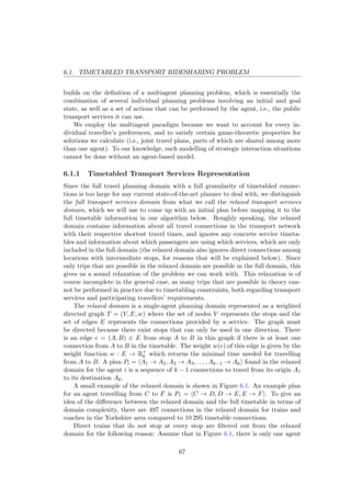
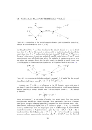
![6.1. TIMETABLED TRANSPORT RIDESHARING PROBLEM
graphs and sets V = n
i=1 Vi, E = n
i=1 Ei, and labels every edge e = (A, B) ∈ E
with the numbers of agents that are using the edge by a labelling function l : V ×
V → 2N . As an example, following Figure 6.1, the merged plan of plans of agent 1
travelling from C to F and sharing a journey from D to E with agent 2 would be
computed as
C → D, D → E, E → F ∪ D → E = {C
{1}
−−→ D
{1,2}
−−−→ E
{1}
−−→ F}
With this, the full domain is represented as a labelled directed multigraph T =
(V , Et, l, l ) where the set of nodes V represents the stops that are present in the
merged plan P of plans from the relaxed domain. A set of edges Et represents the
journey services from the timetable. The labelling function l : Et → s, tA, τ returns
a triple of a unique service name s, a departure time tA from stop A, and a duration
τ of the service journey between stops A and B for each edge e = (A, B) ∈ Et. The
labelling function l : V × V → 2N labels every edge e ∈ E with the number of
agents using it.
A joint plan π with a timetable is a sequence π = a1 . . . ak of joint actions. Each
joint action aj from π represents a subset Nj ⊆ N of agents travelling together using
a specific service sj.
In the example of the full domain in Figure 6.2, the agents can travel using some
subset of five different services S1 to S5. The full domain example is based on the
group of agent 1 (travelling from C to F) and agent 2 (travelling from D to E) where
initial single-agent plans have been found in the relaxed domain shown in Figure 6.1.
In order to travel from C to D using service S1, an agent must be present at stop C
before the departure of service S1 to D.
6.1.2 Multiagent Planning Problem
To model the ridesharing problem, we use a multiagent planning formalism which is
based on MA-STRIPS [12] and coalition-planning games [13]. States are represented
by sets of ground fluents, actions are tuples a = pre(a), eff (a) . These fluents are
logical propositions describing aspects of the current state that may change over time,
e.g., at(1, l1 ) to express that agent 1 is at location l1. After the execution of action
a, positive fluents p from eff (a) are added to the state and negative fluents ¬p are
deleted from the state. For example, an action travel(A, X , Y ), when applied to the
case of A = 1 travelling from X = l1 to Y = l2 would make at(1, l1 ) false and
at(1, l2 ) true. Each agent has individual goals and actions with associated costs.
There is no extra reward for achieving the goal, the total utility received by an agent
is simply the inverse of the cost incurred by the plan executed to achieve the goal. In
the ridesharing domain, the agents are the travellers, located in their origin locations
in the initial state, and attempting to achieve goal states where they are at their
destination locations. Agents specify the initial state and the goal state but their
journey plans are computed for them centrally.
69](https://image.slidesharecdn.com/5227de32-e56f-4573-b73a-9a28ea360750-170109080048/85/dissertation_hrncir_2016_final-77-320.jpg)
![6.1. TIMETABLED TRANSPORT RIDESHARING PROBLEM
More formally, following the notation of [72], a multiagent planning problem is
a tuple
Π = N, F, I, {Gi}n
i=1, {Ai}n
i=1, Ψ, {ci}n
i=1
where
• N = {1, . . . , n} is the set of agents,
• F is the set of fluents,
• I ⊆ F is the initial state,
• Gi ⊆ F is agent i’s goal,
• Ai is agent i’s action set,
• Ψ : A → {0, 1} is an admissibility function,
• ci : ×n
i=1Ai → R is the cost function of agent i.
A = A1×. . .×An is the joint action set assuming a concurrent, synchronous execution
model, and G = ∧iGi is the conjunction of all agents’ individual goals. The assump-
tion of synchronous action among agents here is an important simplification to make
the problem more tractable. We will see below how it is possible to determine spe-
cific synchronisation points for jointly travelling agents when mapping the problem
to the full timetabling information. A multiagent planning problem typically im-
poses concurrency constraints regarding actions that cannot or have to be performed
concurrently by different agents to succeed which the authors of [72] encode using
an admissibility function Ψ, with Ψ(a) = 1 if the joint action a is executable, and
Ψ(a) = 0 otherwise.
A plan π = a1, . . . , ak is a sequence of joint actions aj ∈ A such that a1 is
applicable in the initial state I (i.e., pre(a1) ⊆ I), and aj is applicable following the
application of a1, . . . , aj−1. We say that π solves the multiagent planning problem Π
if the goal state G is satisfied following the application of all actions in π in sequence.
The cost of a plan π to agent i is given by Ci(π) = k
j=1 ci(aj). Each agent’s
contribution to a plan π is denoted by πi (a sequence of ai ∈ Ai).
6.1.3 Timetabled Transport Ridesharing Problem Definition
The real-world ridesharing domain used in this work is based on the large and complex
public transport network in the UK. An agent representing a passenger is able to use
different modes of transport during its journey: walking, trains, and coaches. The
aim of each agent is to get from its starting location to its final destination at the
lowest possible cost. The cost of an agent’s journey can be based on the weighted
sum of several criteria such as journey duration, ticket price, mode of transport, and
number of agents travelling together.
For the purposes of this work, we will make the assumption that sharing a part
of a journey with other agents is cheaper than travelling alone. While this may not
70](https://image.slidesharecdn.com/5227de32-e56f-4573-b73a-9a28ea360750-170109080048/85/dissertation_hrncir_2016_final-78-320.jpg)
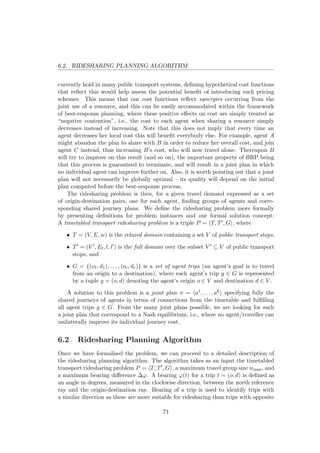
![6.2. RIDESHARING PLANNING ALGORITHM
bearing. The output of the algorithm is a joint plan π = a1, . . . , ak that fulfils all
agent trips g ∈ G.
The main problem when planning for an identified group of agents with a cen-
tralised multiagent planner is the exponential blowup in the action space which is
caused by using concurrent, independent actions [72]. Using a naive PDDL transla-
tion has proven that a direct application of a centralised multiagent planner to this
problem does not scale well. As mentioned above, we tackle the complexity of the
domain by breaking the planning process down into different phases that avoid deal-
ing with the full fine-grained timetable data from the outset. The overall algorithm,
which is shown in Figure 4, is designed to work in four phases, which we will now
describe in detail.
6.2.1 The Trip Grouping Phase
The algorithm starts with the trip grouping phase where the trips G = {(o1, d1), . . . ,
(oc, dc)} are grouped into groups of at most nmax agents. Groups are created incre-
mentally from G, until G becomes empty, in the following way: First, pick a trip
g ∈ G at random. Then, create a set of candidate trips G = {g ∈ G|bd(g, g ) ≤ ∆ϕ}
that have a similar bearing as g (function bd(g, g ) calculates the bearing difference
between trips g and g ). Next, create a group Gj ⊆ G by selecting at most nmax trips
with minimum spatial difference sd(·, g ) to g . Here, the spatial difference sd(g, g )
of two trips g and g is defined as
sd(g, g ) = |o, o | + |d, d |,
where |o, o | denotes the direct distance between the origins of the two trips, and |d, d |
the direct distance between their destinations. Once a group Gj is created, the trips
g ∈ Gj are deleted from the set of all trips G.
For each group Gj, a joint journey plan π with a timetable is found by applying
the next three phases of the algorithm.
6.2.2 The Trip Planning Phase
In the trip planning phase, an initial journey is found for each agent i from the set
of agents Gj using the relaxed domain T = (V, E, w) where the action set is identical
for every agent and contains all transport services available in the transport network.
A journey for each agent is calculated independently of other agents in the scenario
using a single-agent planner. As a result, each agent is assigned a single-agent plan
Pi which will be further optimised in the next phase. This approach makes sense in
our domain because the agents do not need each other to achieve their goals and they
cannot invalidate each other’s plans. A PDDL specification for the relaxed domain
is shown in Section 6.3.
72](https://image.slidesharecdn.com/5227de32-e56f-4573-b73a-9a28ea360750-170109080048/85/dissertation_hrncir_2016_final-80-320.jpg)

![6.2. RIDESHARING PLANNING ALGORITHM
6.2.3 The Best-response Phase
The best-response phase is based on the relaxed domain. Again, the action set is
identical for every agent and contains all transport services available in the transport
network. The algorithm uses the best-response planning algorithm as described be-
low. It iteratively creates and solves simpler best-response planning problems from
the point of view of each individual agent. In the case of the relaxed domain, the
best-response planning problem looks almost the same as a problem of finding a single-
agent journey. The difference is that, as we have explained in Section 6.1.3, we make
the assumption that the cost of travelling is smaller when an agent uses a connection
which is used by one or more other agents. A specific cost function used for the
evaluation of the algorithm is defined in Section 6.4.1.
Iterations over agents continue until there is no change in the cost of the joint plan
between two successive iterations. This means that the joint plan cannot be further
improved using the best-response approach. The purpose of this is not only to exploit
local, “greedy” optimisations for single agents in an overall schedule of plans. It also
ensures that the proposed joint solution is compatible with the incentives of individual
agents, i.e., they could do no better on their own by deviating from it. The fact that
the first iteration of the best-response optimisation starts from initial plans that
agents can perform on their own ensures this (any subsequent plan generated will be
cheaper to them). The output of the best-response phase is a merged plan P of the
single-agent plans in the relaxed domain (defined in Section 6.1.1) that specifies which
connections the agents use for their journeys and which segments of their journeys
are shared. The merged plan P will be matched to the timetable in the final phase
of the algorithm.
Best-response Planning
The best-response planning algorithm proposed in [72] is an algorithm which, given
a solution πk to a multiagent planning problem Π, finds a solution πk+1 to a trans-
formed planning problem Πi with minimum cost Ci(πk+1) for agent i among all pos-
sible solutions, while considering all other agents’ plans to be fixed:
πk+1
= arg min{Ci(π)|π identical to πk
for all j = i}
The transformed planning problem Πi is obtained by rewriting the original problem Π
so that all other agents’ actions are fixed, and agent i can only choose its own actions
in such a way that all other agents still can perform their original actions. Since Πi
is a single-agent planning problem, any cost-optimal planner can be used as a best-
response planner.
In [72], the authors show how for a class of congestion planning problems, where
all fluents are private, the transformation they propose allows the algorithm to con-
verge to a Nash equilibrium if agents iteratively perform best-response steps using
an optimal planner. This requires that every agent can perform its actions with-
out requiring another agent, and hence can achieve its goal in principle on its own,
74](https://image.slidesharecdn.com/5227de32-e56f-4573-b73a-9a28ea360750-170109080048/85/dissertation_hrncir_2016_final-82-320.jpg)
![6.2. RIDESHARING PLANNING ALGORITHM
and conversely, that no agent can invalidate other agents’ plans. Assuming infinite
capacity of vehicles (or, more realistically, large enough capacities to accommodate
at least the number of agents for whom we are trying to find a plan), the relaxed
domain is an instance of a congestion planning problem: following the definition of
a congestion planning problem in [72], all actions are private, as every agent can use
modes of transport on their own and the other agents’ concurrently taken actions
only affect action cost. The convergence of the best-response phase derives from the
theorem presented in [72] which states that for any congestion planning problem,
best-response planning converges to a pure-strategy Nash equilibrium.
The best-response planner works in two phases: In the first phase, an initial plan
for each agent is computed (e.g., each agent plans independently or a centralised
multiagent planner is used). In the second phase, the planner solves simpler best-
response planning problems from the point of view of each individual agent. The
goal of the planner in a best-response planning problem is to minimise the cost of
an agent’s plan without changing the plans of others (though the cost of their plans
might change as explained in Section 6.1.3). Consequently, it optimises a plan of each
agent with respect to the current joint plan.
This approach has several advantages. It supports full concurrency of actions and
the best-response phase avoids the exponential blowup in the action space resulting
in much improved scalability. For the class of potential games [79], it guarantees
convergence to a Nash equilibrium. On the other hand, it does not guarantee the op-
timality of a solution, i.e., the quality of the equilibrium in terms of overall efficiency
is not guaranteed (it depends on which initial plan the agents start off with). How-
ever, experiments have proven that it can be successfully used for improving general
multiagent plans [72].
6.2.4 The Timetabling Phase
In the final timetabling phase, the optimised shared journeys are matched against
timetables using a temporal single-agent planner which assumes the full domain. For
this, in a first step, independent groups of agents with respect to journey sharing are
identified. An independent group of agents is defined as an edge disjoint subgraph
of the merged plan P. This means that actions of independent groups do not affect
each other so it is possible to find a timetable for each independent group separately.
Then, for every independent group, parts of the group journey are identified.
A part of the group journey is defined as a maximal continuous segment of the group
journey which is performed by the same set of agents. As an example, there is a group
of two agents that share a segment of their journeys in Figure 6.3: Agent 1 travels
from A to G while agent 2 travels from B to H. Their group journey has five parts,
with the shared part (part 3) of their journey occurring between stops C and F.
In order to use both direct and stopping trains when the group journey is matched
to the timetable, the relevant timetable for a group journey is composed in the fol-
lowing way: for every part of the group journey, return all timetable services in the
direction of agents’ journeys which connect the stops in that part. An example of
75](https://image.slidesharecdn.com/5227de32-e56f-4573-b73a-9a28ea360750-170109080048/85/dissertation_hrncir_2016_final-83-320.jpg)
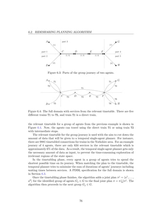
![6.3. RIDESHARING PLANNING ALGORITHM IMPLEMENTATION
6.3 Ridesharing Planning Algorithm Implementation
This section describes two important aspects of the ridesharing planning algorithm
implementation. It deals with the conversion of public transport timetables data
to the Planning Domain Definition Language and with the choice of planners for
implementing the individual phases of the algorithm.
To be able to use timetables data of public transport services with modern AI
planning systems, it has to be converted to the Planning Domain Definition Language
(PDDL). We transformed the data in three subsequent stages. First, we transformed
the NPTDR and NaPTAN XML data to a spatially-enabled PostgreSQL database.
Second, we automatically processed and optimised the data in the database. The data
processing by SQL functions in the procedural PL/pgSQL language included the fol-
lowing steps: merging bus bays at bus stations and parts of train stations, introducing
walking connections to enable multimodal journeys, and eliminating duplicates from
the timetable. Finally, we created a script for generating PDDL specifications based
on the data in the database. More details about the data processing and PDDL
specifications can be found in [62].
(define (domain travelplanner)
(:requirements :typing :action-costs)
(:types location)
(:predicates
(connection ?origin - location ?destination - location)
(at ?loc - location)
)
(:functions
(time ?origin - location ?destination - location)
(total-cost)
)
(:action go
:parameters (?o ?d - location)
:precondition (and (at ?o) (connection ?o ?d) )
:effect (and
(at ?d) (not (at ?o))
(increase (total-cost) (time ?o ?d)) )
)
)
Figure 6.5: The domain file for the relaxed domain.
In the relaxed domain used in the trip planning and best-response phase, a single
agent aims to travel from its origin to its destination. The domain file contains
two predicates, two functions and only one action, cf. Figure 6.5. The predicate
connection is true when there is an edge from ?origin to ?destination (there
are separate edges for walking, travel by bus or train), the predicate at denotes the
current location of the agent. The function time returns the cost of travelling from
the location ?origin to ?destination. The action go moves the agent from the
location ?o to ?d and it increases the total cost of the plan which is stored by the
total-cost function. The problem file then contains the origin and destination of
77](https://image.slidesharecdn.com/5227de32-e56f-4573-b73a-9a28ea360750-170109080048/85/dissertation_hrncir_2016_final-85-320.jpg)
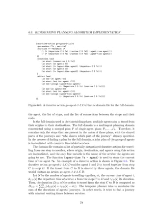
![6.4. RIDESHARING PLANNING ALGORITHM EVALUATION
The conditions of the action are the following: there must be a connection by
the service s between the stops C, D and the agents must be present at the stop C
before the departure of service s. Once the action is executed, the agents are located
at stop D and their current time is set to the arrival of the service s at stop D. The
problem file contains origins and destinations of the agents and the list of services
and their departures and durations.
6.3.1 Planners
All three single-agent planners used for the implementation were taken from recent
International Planning Competitions from 2008 and 2011. We use LAMA [93] in
the trip planning phase and for each of the individual single-agent best-response
iterations in the best-response phase. LAMA is a sequential satisficing (as opposed
to cost-optimal) planner which searches for any plan that solves a given problem
and does not guarantee optimality of the plans computed. LAMA is a propositional
planning system based on heuristic state-space search. Its core feature is the usage
of landmarks, i.e., propositions that must be true in every solution of a planning
problem.
SGPlan6 [69] and POPF2 [18] are the two temporal satisficing planners used in
the timetabling phase. Such temporal planners take the duration of actions into
account and try to minimise makespan (i.e., total duration) of a plan but do not
guarantee optimality. The two planners use different search strategies and usually
produce different results. This allows us to run them in sequence on every problem
and to pick the plan with the shortest duration. It is not strictly necessary to run
both planners, one could save computation effort by trusting one of them.
In many of the experiments, the SGPlan6 and POPF2 used in the timetabling
phase returned some plans in the first minute but then they continued exploration of
the search space without returning any better plan. To account for this, we imposed
a time limit for each planner in the temporal planning stage to 2 minutes for a group
of up to 4 agents and 4 minutes otherwise.
6.4 Ridesharing Planning Algorithm Evaluation
We have evaluated the proposed ridesharing algorithm on realistic scenarios based
on real-world public transport timetables and travel demand data for the Yorkshire
area of the United Kingdom. The size of the area was dictated solely by our need to
evaluate the algorithm on the whole travel demand (approximately 100000 train trips
per day). The ridesharing planning algorithm itself scales up well up to the area of
the whole UK, as was shown in our previous work [64]. However, there the algorithm
was evaluated on travel demand that was very sparsely and randomly sampled, not
necessarily showing any correlation to actual travel demand profiles.
79](https://image.slidesharecdn.com/5227de32-e56f-4573-b73a-9a28ea360750-170109080048/85/dissertation_hrncir_2016_final-87-320.jpg)
![6.4. RIDESHARING PLANNING ALGORITHM EVALUATION
6.4.1 Experiment Settings
The experiments are situated in the Yorkshire area (East and West Yorkshire, East
Riding of Yorkshire, York, and Selby administrative areas) which covers an area of
approximately 130 by 70 km, i.e., around 9 100 km2. According to the UK origin-
destination census data from 2001 [86], there are 2 million passenger trips a day in
the Yorkshire area. In order to focus on the timetabled public transport trips, the
modal split in the UK across different modes of transport in 2001 [42] was used to
estimate the number of trips for each mode, cf. Table 6.1.
Table 6.1: Numbers of trips per day in the Yorkshire area [42, 86].
Transport mode Modal split 100% trips 50% trips 5% trips
Trains 5.3% 106 035 53 017 5 302
Coaches 0.3% 6 002 3 001 300
Local buses 6.0% 120 039 60 020 6 002
Passenger cars 88.3% 1 766 576 883 288 88 329
Total 100.0% 1 998 651 999 326 99 933
Since we assume that all agents are travelling on the same day and that all journeys
must be completed within 24 hours, in what follows below we consider only public
transport timetables data for Tuesdays (this is an arbitrary choice that could be
changed without any problem).
The timetable data used in this work contains neither information about ticket
prices nor distances between adjacent stops, only durations of journeys from one stop
to another. This significantly restricts the design of a cost functions used for the
planning problems. Therefore, the cost functions used in this work are based solely
on the duration of journeys. The cost ci,n for agent i travelling from A to B in a group
of n agents is then defined by equation (6.1):
ci,n = 1
n 0.8 + 0.2 ci (6.1)
where ci is the individual cost of the single action to i when travelling alone. In this
work, we take this to be equal to the duration of the journey from A to B.
This is designed to approximately model the discount for the passengers if they
buy a group ticket: The more agents travel together, the cheaper the shared (leg of a)
journey becomes for each agent. Also, an agent cannot travel any cheaper than 20%
of the single-agent cost. In reality, pricing for group tickets could vary, and while our
experimental results assume this specific setup, the actual price calculation could be
easily replaced by any alternative model.
The experiments are based on running the algorithm on one core of a 3.2 GHz Intel
Core i7 processor of a Linux desktop computer. The data, source code, and scenarios
in PDDL for the timetabled transport ridesharing problem are openly available in
a repository1 under LGPL license2.
1
https://github.com/agents4its/ridesharingontimetabledtransport
2
http://www.gnu.org/licenses/lgpl.html
80](https://image.slidesharecdn.com/5227de32-e56f-4573-b73a-9a28ea360750-170109080048/85/dissertation_hrncir_2016_final-88-320.jpg)
![6.4. RIDESHARING PLANNING ALGORITHM EVALUATION
6.4.2 Experiment Scenarios
We used the following parameters as factors in experiment scenarios: (1) travel de-
mand generation; (2) ridesharing demand proportion; (3) modes of transport consid-
ered; (4) maximum travel group size. The values of the parameters are summarised
in Table 6.2. We set the maximum bearing difference parameter of the algorithm to
∆ϕ = 25 degrees for all scenarios.
Table 6.2: Experiment scenarios parameters overview.
Scenario parameter Parameter values
Travel demand generation {realistic, random}
Ridesharing demand proportion {100%, 50%, 5%}
Modes of transport {trains only, trains and coaches}
Maximum travel group size {2, 4, 6, 8}
Travel Demand Generation. We use two types of travel demand. The realistic
travel demand generation is based on the UK census 2001 origin-destination data [86]
that contains numbers of trips carried out from every origin district to every other
destination district. District-to-district trip counts are mapped to stop-to-stop trip
counts in the following way: For each origin-destination district pair, the desired
number of trips is generated randomly from the Cartesian product of stops in the
origin and destination district. Since the UK census origin-destination data is not
provided at the level of granularity required to select concrete stops in the travel
network, we have sampled these within each district with probability proportional to
the density of services passing through a stop. This is based on the assumption that
service density roughly follows numbers of travellers using a stop. In addition to the
realistic demand, we also experimented using random travel demand generated ran-
domly from the Cartesian product of stops in the Yorkshire area, assuming a uniform
distribution over stops.
From the travel demand distribution generated, only trips with a straight-line
distance between the origin and the destination in the interval 25–100 km are used for
the evaluation (when using roads or rail tracks, this interval stretches approximately
to a real distance of 40–160 km). This interval was chosen to filter out trips that are
too short to be planned in advance and therefore not very suitable for sharing. This
led to the removal of 86% of all trips in the realistic travel demand generation process
and to the removal of 30% of all trips in the random travel demand generation process.
Ridesharing Demand Proportion. In order to observe the behaviour of the sys-
tem with different densities of trips we set the portion of travel demand to 100%,
50%, and 5% of the total number of trips.
Modes of Transport. In order to evaluate the behaviour of the algorithm on both
a unimodal and a multimodal public transport network, trains only and a combination
of trains and coaches were used in the experiments. In the Yorkshire area, there are
150 (201) stops, 330 (495) connections in the relaxed domain, and 9 881 (10 289)
81](https://image.slidesharecdn.com/5227de32-e56f-4573-b73a-9a28ea360750-170109080048/85/dissertation_hrncir_2016_final-89-320.jpg)
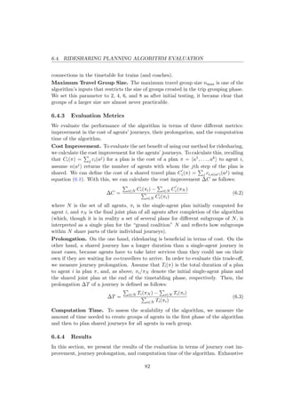
![6.4. RIDESHARING PLANNING ALGORITHM EVALUATION
0
10
20
30
40
50
60
70
2 4 6 8
costimprovement[%]
maximum group size
5% trips
50% trips
100% trips
0
5
10
15
20
25
30
2 4 6 8
prolongation[%] maximum group size
5% trips
50% trips
100% trips
Figure 6.7: Average cost improvement and prolongation against maximum group size
(realistic travel demand, trains and coaches).
experiment design was used; all metrics were evaluated for all combinations of all val-
ues of all scenario parameters. Specifically, for each type of travel demand generation,
we tested all combinations of modes of transport, and for each ridesharing demand
proportion, we generated the travel demand. Then for each maximum group size,
the whole travel demand is an input for the algorithm which in its trip grouping
phase creates the groups of agents for ridesharing. From the set of all groups cre-
ated, a detailed journey plan with a timetable is found in the last three phases of the
algorithm for a sample of 80 randomly chosen groups (sampling was performed to
reduce experiment computational time while maintaining significance of the results).
Each possible experiment configuration is averaged over 8 stochastic travel demand
generation instances. This leads to an overall number of 30 720 groups of agents over
which the algorithm was evaluated.
Cost Improvement. The average cost improvement obtained in our experiments
is shown in Figure 6.7. It shows that the more agents are grouped together in the
trip grouping phase of the algorithm, the higher the improvement. These results
were obtained based on the specific cost function (6.1) we have introduced to favour
ridesharing, and which would have to be adapted to the specific cost structure that is
present in a given transport system. Also, the extent to which longer journey times
are acceptable for the traveller depends on their preferences, but these could be easily
adapted by using different cost functions.
Prolongation. The average prolongation of journeys is shown in Figure 6.7 where
8% of groups with prolongation greater than 100% is filtered out from the average
calculation (these are the journeys which, though feasible, are unlikely to be accepted
by travellers). The graph shows that the more agents are grouped together in the
trip grouping phase of the algorithm, the higher the prolongation. Furthermore, the
prolongation with the 5% ridesharing proportion is much higher then when consider-
83](https://image.slidesharecdn.com/5227de32-e56f-4573-b73a-9a28ea360750-170109080048/85/dissertation_hrncir_2016_final-91-320.jpg)
![6.4. RIDESHARING PLANNING ALGORITHM EVALUATION
0
10
20
30
40
50
60
70
0 20 40 60 80 100
costimprovement[%]
prolongation [%]
(a) 5% trips
0
10
20
30
40
50
60
70
0 20 40 60 80 100
costimprovement[%]
prolongation [%]
(b) 50% trips
Figure 6.8: Cost improvement against prolongation (realistic travel demand, trains
and coaches, maximum group size nmax = 4).
ing 50% or 100% ridesharing proportion. As the density of trips drops, the agents in
groups are more spatially dispersed, which causes higher relative prolongation ratios.
Figure 6.8 shows a scatter plot of cost improvement versus prolongation for in-
dividual trips for 5% and 50% ridesharing proportion. It can be observed that with
a higher ridesharing proportion, the majority of the groups has either prolongation
very close to 0% (identical trips are shared) or has a very high cost improvement
(between 50% and 60%). With a lower ridesharing proportion, there are many more
groups with lower cost improvement or higher prolongation. What is encouraging is
that even for small populations of potential ridesharers, there are many shared jour-
neys with a good cost improvement and a reasonable prolongation. In our algorithm,
the balance between the two criteria could be calibrated by changing the weights in
the cost function.
Computation Time. The first graph in Figure 6.9 shows the overall computation
times of the algorithm for one created group of agents from the realistic demand and
a combination of trains and coaches. The trip grouping phase of the algorithm is
very fast (200 ms per group on average). The algorithm spends the majority of the
computation time solving the problem of finding a joint plan for the group of agents.
The graph indicates that the overall computation time grows roughly linearly with
increasing numbers of agents in a group, which confirms that the algorithm avoids
the exponential blowup in the action space characteristic for centralised multiagent
planning. This is mainly a consequence of the best-response planning algorithm, and
an expected result.
The second graph in Figure 6.9 shows the overall computation times of the algo-
rithm for one created group of agents from the random demand and for a combination
of trains and coaches. It can be observed that the algorithm is faster at the realistic
84](https://image.slidesharecdn.com/5227de32-e56f-4573-b73a-9a28ea360750-170109080048/85/dissertation_hrncir_2016_final-92-320.jpg)
![6.4. RIDESHARING PLANNING ALGORITHM EVALUATION
0
20
40
60
80
100
120
140
160
180
2 4 6 8
runtime[s]
maximum group size
5% trips
50% trips
100% trips
(a) Realistic travel demand
0
20
40
60
80
100
120
140
160
180
2 4 6 8
runtime[s] maximum group size
5% trips
50% trips
100% trips
(b) Random travel demand
Figure 6.9: Computation time against maximum group size (trains and coaches).
5% ridesharing proportion than for random trips. At the 50% and 100% ridesharing
proportion, there is not a very big difference between the computation times. This
suggests that the trips from the realistic 5% ridesharing proportion reflects the public
transport network making the journey planning easier whereas it is harder to plan
for trips distributed randomly.
Regarding the modes of transport in the scenario, it is harder to find joint plans
when a combination of trains and coaches is considered (on average, runtimes are
25% higher for scenarios with trains and coaches). Considering a combination of
trains and coaches does not significantly affect neither the cost improvement, nor the
prolongation.
While the overall computation times are considerable (up to 2 minutes for a group
of 8 agents from the realistic 5% ridesharing proportion), we should emphasise that
the algorithm is effectively computing equilibrium solutions in multi-player games
with hundreds of thousands of states. Considering this, the linear growth hints at
having achieved a level of scalability based on the structure of the domain that is far
above naive approaches to plan jointly in such state spaces.
Finally, we have evaluated the overall computation time for all trips from the travel
demand. We were able to compute shared journey plans for approximately 13 500
trips from realistic 100% ridesharing proportion when considering a combination of
trains and coaches. It took less than 75 minutes for each setting of maximum group
size while using 8 cores of 3.2 GHz Intel Core i7 processor on three computers in
parallel.
The ridesharing algorithm can be further parallelised down to a level of individual
groups, bringing the computation time to few minutes for the whole demand. This
follows from the structure of the algorithm: In the trip planning phase, the identi-
fication of initial single-agent plans for the travellers consists of a set of completely
85](https://image.slidesharecdn.com/5227de32-e56f-4573-b73a-9a28ea360750-170109080048/85/dissertation_hrncir_2016_final-93-320.jpg)
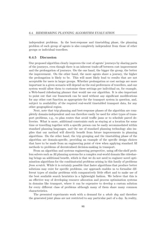
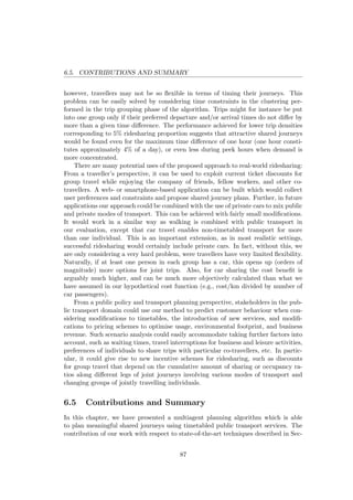
![6.5. CONTRIBUTIONS AND SUMMARY
tion 2.5 is threefold:
Firstly, we have applied state-of-the-art automated planning techniques to real-
world public transport data to evaluate their feasibility in this domain. This allows to
consider the inclusion of multimodal public transport services in ridesharing activities
and to explore opportunities to combine their use with private cars in the future. In
addition to serving as a basis for traveller-oriented ridesharing service, our system
allows stakeholders to determine appropriate pricing policies to incentivise group
travel and to predict the effects of potential service changes.
Secondly, we have presented an algorithm that combines different techniques in
a practically-oriented way and works with real-world public transport timetables
and realistic travel demand even though it is largely based on extensible, domain-
independent, off-the-shelf heuristic problem solvers. The four-phase algorithm utilises
performant single-agent planners to find individual plans in a simplified domain first
and then merges them using a best-response planner which ensures resulting solutions
are individually rational.
Thirdly, the algorithm has been implemented and evaluated on realistic scenar-
ios based on real-world UK transport data. In the process, we have described the
engineering steps that are necessary to deal with the challenges of real-world large-
scale data and propose suitable solutions. Experiments with realistic travel demand
show that, for a wide range of scenarios, the algorithm is capable of finding shared
journeys with very attractive trade-offs between cost saving and journey time pro-
longation. The algorithm exhibits very good scalability. It scales linearly with the
number of trips processed, regardless of the size of travel groups considered. The al-
gorithm is also amenable to massive parallelisation which can bring the time required
for planning shared journeys for real-world travel demand down to minutes.
The model for the timetabled transport ridesharing problem, the ridesharing plan-
ning algorithm, and the evaluation of the algorithm has been designed in collaboration
with Michael Rovatsos. Michael has also contributed to related work regarding mul-
tiagent trip planning in Section 2.5. Finally, this topic has been published in the
following articles [64, 65].
88](https://image.slidesharecdn.com/5227de32-e56f-4573-b73a-9a28ea360750-170109080048/85/dissertation_hrncir_2016_final-96-320.jpg)
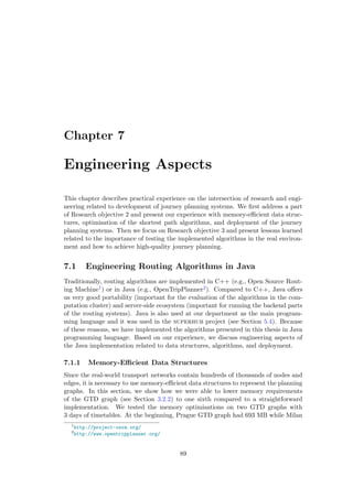
![7.1. ENGINEERING ROUTING ALGORITHMS IN JAVA
GTD graph had 1218 MB using the straightforward representation. In the following
list, we describe the key optimisations we have performed:
• Initially, we used a long identifier for each node that corresponded to the OSM
identifier. The disadvantage was that the identifiers of the nodes did not consti-
tute an increasing sequence. We have improved this by switching to an integer
identifier and having node identifiers from 0 to |V | − 1 where |V | is the number
of nodes in the graph. This enabled us to use arrays instead of maps in the
representation of the graph.
• In the graph object, we have replaced Map<Long, TNode> with nodes represen-
tation in ArrayList<TNode>.
• We have improved the representation of outgoing edges by replacing Map<Long,
List<TEdge>> with edge list ArrayList<TEdge> and int[] representing start-
ing positions in the edge list for the adjacency list of each node.
• Each edge in the GTD graph is annotated with the allowed modes of trans-
port. We have encoded the Set<ModeOfTransport> into a single int using bit
operations.
• In the straightforward implementation of the PT timetables, we have used
TreeSet<Departure> to capture all departures on a route edge (defined in Sec-
tion 3.2.1). Each Departure object contained a DateTime object for departure
time and int for the duration. With the defined comparator for the Departure,
it was possible to call higher method of the TreeSet to get easily the next de-
parture given a specified time. We have replaced this with int[] to capture the
departures now represented as seconds from the start of the timetable validity.
In addition, if all the durations on the route edge are the same, we use just one
int to capture the duration; otherwise we use single int to specify duration for
each departure on the route edge as before.
After performing the listed improvements, we measured the memory consumption
again. We managed to lower the memory size of Prague GTD graph to 113 MB (16%
of the original size) and the memory size of Milan GTD graph to 220 MB (18% of
the original size). In conclusion, the data structures need to be carefully designed
to capture urban-scale GTD graphs with the minimum amount of memory and to
enlarge the graphs to country-scale in the future.
7.1.2 Heaps Choice for Shortest Path Algorithms
There are several points where the implementation of shortest path algorithms can
be fine-tuned. In this section, we discuss the choice of a heap for the Dijkstra’s
and A* algorithms. There are two main candidates: Fibonacci heap and binomial
heap. The main operations used during the search are insert, decrease key, and delete
the minimum. In theory, the Fibonacci heap has a better time complexity then the
90](https://image.slidesharecdn.com/5227de32-e56f-4573-b73a-9a28ea360750-170109080048/85/dissertation_hrncir_2016_final-98-320.jpg)
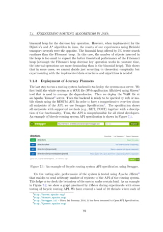
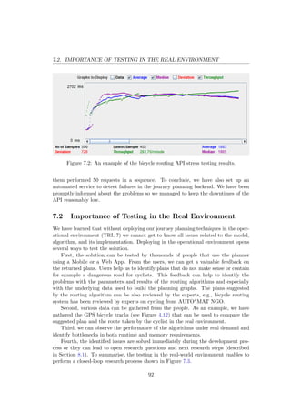
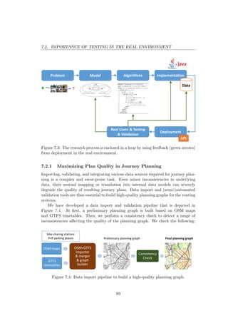
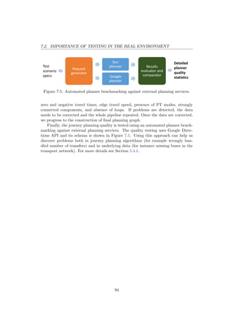
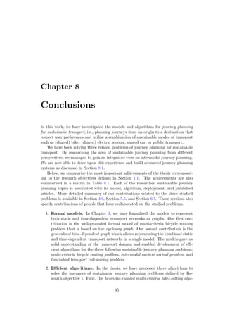
![Table 8.1: Thesis achievements matrix.
Multi-Criteria
Bicycle Routing
(Chapter 4)
Intermodal
Journey Planning
(Chapter 5)
Ridesharing
on Timetabled
Transport Services
(Chapter 6)
Formal models
Cycleway Graph
(Section 3.1.2)
Generalised
Time-dependent
Graph
(Section 3.2.2)
Relaxed and Full
Transport Services
Domain
Multi-Criteria
Bicycle Routing
Problem
Intermodal Earliest
Arrival Problem
Timetabled Transport
Ridesharing Problem
Efficient
algorithms
HMLS Algorithm
with Speedups
Intermodal
Planning Algorithm
Ridesharing
Planning Algorithm
Validation
in real-world
deployments
Bicycle Routing
System
Intermodal Journey
Planning System
-
Published in [66, 67, 68, 103] [63, 71] [64, 65]
rithm together with a combination of heuristics solves the multi-criteria bicy-
cle routing problem. Second, the intermodal planning algorithm using a gen-
eralised time-dependent graph structure solves the intermodal earliest arrival
problem. Finally, the ridesharing planning algorithm using state-of-the-art au-
tomated planning techniques solves the timetabled transport ridesharing prob-
lem. Findings related to memory-efficient data structures and implementation
of the algorithms are discussed in Section 7.1. All implemented algorithms for
sustainable journey planning has been thoroughly evaluated in an exhaustive
set of experiments using real-world map and PT timetables data. Runtime of
the algorithms, quality of returned plans and other metrics have been measured,
presented, and discussed.
3. Validation in real-world deployments. Finally, in Section 4.5 and Sec-
tion 5.4, we have presented how the Bicycle Routing System and Intermodal
Journey Planning System have been validated in real-world deployments with
real users. It has been validated that the systems are capable of working in an
operational environment (TRL 7) and they have the potential to help people
with the navigation on their urban journeys. Based on deployments, we have
also summarised engineering aspects of developing journey planning systems in
Chapter 7. The key lessons learned are related to testing in real environment
and the need for high-quality planning graphs. The experience is valuable with
respect to the future work in the sustainable journey planning field.
96](https://image.slidesharecdn.com/5227de32-e56f-4573-b73a-9a28ea360750-170109080048/85/dissertation_hrncir_2016_final-104-320.jpg)
![8.1. FUTURE WORK
8.1 Future Work
In this section, we list several directions worth exploring in the future that has
emerged during the work on the thesis. We conclude this section by looking more
ahead to the trend of seamless door-to-door mobility that can be supported by our
work on journey planning for sustainable transport.
The multi-criteria search often produces large Pareto sets with many similar
routes. We therefore plan to provide a filtering method (e.g., based on our preliminary
work that uses clustering [103]) that would select several representative routes from
a potentially very large set of Pareto routes. This will be useful for the multi-criteria
bicycle routing problem as well as for the use of multi-criteria search in intermodal
journey planning.
We aim to incorporate real-world GPS tracks we have been collecting into the
routing process (e.g., according to [29]). This should further improve the quality of
route suggestions by making it possible to consider route-choice factors that cannot be
reflected based solely on the underlying map data. Furthermore, comparing real-world
GPS tracks with the transport network graph is a powerful way of (semi-)automated
detection of problems in transport network data.
In order to deliver high-quality journey plans to users, it is necessary to build jour-
ney planning systems on top of high-quality planning graphs that represent transport
networks. Based on our experience, importing, validating, and integrating various
data sources required for journey planning is a complex and error-prone task. In
addition, the transport network changes over time, e.g., new cycleways are built or
PT timetables are updated. We would like to extend our data import and validation
pipeline (described in Section 7.2.1) to an automated tool that would build, validate,
and also maintain a high-quality planning graph.
In the long run, we would like to contribute to the concept of seamless door-to-
door mobility where the users are provided with intelligent journey planning tools
that arrange the whole door-to-door journey. Importantly, this concept employs re-
source allocation for automated seat reservation and ticket purchase using booking
and ticketing APIs provided by mobility services operators. We have started to ex-
plore this concept by researching the combination of several existing journey planner
APIs to deliver intermodal journey planning functionality [83]. We could also use our
experience with ridesharing to enable seamless door-to-door ridesharing.
In the thesis, we have made scientific contributions to solving several journey
planning problems. Equally importantly, we have demonstrated that our scientific
results can be translated into real-world solutions, which can ultimately facilitate the
critically needed shift towards sustainable mobility.
97](https://image.slidesharecdn.com/5227de32-e56f-4573-b73a-9a28ea360750-170109080048/85/dissertation_hrncir_2016_final-105-320.jpg)
![Bibliography
[1] Mobility 2001: World Mobility at the End of the Twentieth Century and Its
Sustainability. Technical report, Massachusetts Institute of Technology and
Charles River Associated Incorporated, 2001.
[2] H. Bast. Car or Public Transport – Two Worlds. In S. Albers, H. Alt, and S. Na-
her, editors, Efficient Algorithms, volume 5760 of Lecture Notes in Computer
Science, pages 355–367. Springer Berlin Heidelberg, 2009.
[3] H. Bast, M. Brodesser, and S. Storandt. Result Diversity for Multi-Modal
Route Planning. In 13th Workshop on Algorithmic Approaches for Transporta-
tion Modelling, Optimization, and Systems (ATMOS), pages 123–136, Sophia
Antipolis, France, 2013.
[4] H. Bast, E. Carlsson, A. Eigenwillig, R. Geisberger, C. Harrelson, V. Raychev,
and F. Viger. Fast Routing in Very Large Public Transportation Networks Using
Transfer Patterns. In M. Berg and U. Meyer, editors, European Symposium on
Algorithms (ESA), volume 6346 of Lecture Notes in Computer Science, pages
290–301. Springer Berlin Heidelberg, 2010.
[5] H. Bast, D. Delling, A. V. Goldberg, M. Muller-Hannemann, T. Pajor,
P. Sanders, D. Wagner, and R. F. Werneck. Route planning in transporta-
tion networks. CoRR, 2015.
[6] H. Bast, S. Funke, D. Matijevic, P. Sanders, and D. Schultes. In Transit to Con-
stant Time Shortest-Path Queries in Road Networks. In Meeting on Algorithm
Engineering and Experiments (ALENEX). SIAM, 2007.
[7] H. Bast, S. Funke, P. Sanders, and D. Schultes. Fast Routing in Road Networks
with Transit Nodes. Science, 316(5824), 2007.
[8] R. Bauer and D. Delling. SHARC: Fast and robust unidirectional routing. ACM
Journal of Experimental Algorithmics, 14, 2009.
[9] R. Bauer, D. Delling, and D. Wagner. Experimental study of speed up tech-
niques for timetable information systems. Networks, 57(1):38–52, 2011.
[10] G. Berbeglia, J. F. Cordeau, and G. Laporte. Dynamic pickup and delivery
problems. European Journal of Operational Research, 202(1):8–15, 2010.
98](https://image.slidesharecdn.com/5227de32-e56f-4573-b73a-9a28ea360750-170109080048/85/dissertation_hrncir_2016_final-106-320.jpg)
![BIBLIOGRAPHY
[11] C. Boutilier and R. Brafman. Partial-order planning with concurrent interacting
actions. Journal of Artificial Intelligence Research, 14:105–136, 2001.
[12] R. Brafman and C. Domshlak. From One to Many: Planning for Loosely Cou-
pled Multi-Agent Systems. In International Conference on Automated Planning
and Scheduling (ICAPS), pages 28–35. AAAI Press, 2008.
[13] R. Brafman, C. Domshlak, Y. Engel, and M. Tennenholtz. Planning Games. In
International Joint Conference on Artificial Intelligence (IJCAI), volume 21,
pages 73–78, 2009.
[14] J. Broach, J. Dill, and J. Gliebe. Where do cyclists ride? A route choice model
developed with revealed preference GPS data. Transportation Research Part A:
Policy and Practice, 46(10):1730–1740, 2012.
[15] G. S. Brodal and R. Jacob. Time-dependent Networks as Models to Achieve Fast
Exact Time-table Queries. Electronic Notes in Theoretical Computer Science,
92:3–15, 2004.
[16] I. Carreras, S. Gabrielli, D. Miorandi, A. Tamilin, F. Cartolano, M. Jakob,
and S. Marzorati. SUPERHUB: A user-centric perspective on sustainable ur-
ban mobility. In 6th ACM workshop on Next generation mobile computing for
dynamic personalised travel planning, pages 9–10. ACM, 2012.
[17] V. Codina, J. Mena, and L. Oliva. Context-aware user modeling strategies
for journey plan recommendation. In F. Ricci, K. Bontcheva, O. Conlan, and
S. Lawless, editors, User Modeling, Adaptation and Personalization, volume
9146 of Lecture Notes in Computer Science, pages 68–79. Springer International
Publishing, 2015.
[18] A. J. Coles, A. I. Coles, M. Fox, and D. Long. POPF2: a Forward-Chaining
Partial Order Planner. In International Planning Competition (IPC), 2011.
[19] K. L. Cooke and E. Halsey. The shortest route through a network with time-
dependent internodal transit times. Journal of Mathematical Analysis and Ap-
plications, 14:493–498, 1966.
[20] J. F. Cordeau and G. Laporte. The dial-a-ride problem: models and algorithms.
Annals of Operations Research, 153(1):29–46, 2007.
[21] D. W. Corne. The good of the many outweighs the good of the one: evolutionary
multi-objective optimization. In IEEE Connections Newsletter, pages 9–13.
IEEE, 2003.
[22] J. Cox and E. Durfee. An efficient algorithm for multiagent plan coordination.
In International Conference on Autonomous Agents and Multiagent Systems
(AAMAS), pages 828–835, Utrecht, The Netherlands, 2005.
99](https://image.slidesharecdn.com/5227de32-e56f-4573-b73a-9a28ea360750-170109080048/85/dissertation_hrncir_2016_final-107-320.jpg)
![BIBLIOGRAPHY
[23] J. Cox and E. Durfee. Efficient and distributable methods for solving the multi-
agent plan coordination problem. Multiagent and Grid Systems, 5(4):373–408,
2009.
[24] M. de Weerdt and B. Clement. Introduction to planning in multiagent systems.
Multiagent and Grid Systems, 5(4):345–355, 2009.
[25] B. C. Dean. Continuous-time dynamic shortest path algorithms. Master’s
thesis, Massachusetts Institute of Technology, 1999.
[26] D. Delling, J. Dibbelt, T. Pajor, D. Wagner, and R. F. Werneck. Computing
and Evaluating Multimodal Journeys. Technical Report 2012-20, Faculty of
Informatics, Karlsruhe Institut of Technology, 2012.
[27] D. Delling, J. Dibbelt, T. Pajor, D. Wagner, and R. F. Werneck. Computing
Multimodal Journeys in Practice. In International Symposium on Experimental
Algorithms, pages 260–271, 2013.
[28] D. Delling, J. Dibbelt, T. Pajor, and R. Werneck. Public transit labeling. In
E. Bampis, editor, Experimental Algorithms, volume 9125 of Lecture Notes in
Computer Science, pages 273–285. Springer International Publishing, 2015.
[29] D. Delling, A. Goldberg, M. Goldszmidt, J. Krumm, K. Talwar, and R. Wer-
neck. Navigation Made Personal: Inferring Driving Preferences from GPS
Traces. In 23rd International Conference on Advances in Geographic Infor-
mation Systems (ACM SIGSPATIAL). ACM Press, 2015.
[30] D. Delling, A. Goldberg, and R. Werneck. Hub label compression. In V. Boni-
faci, C. Demetrescu, and A. Marchetti-Spaccamela, editors, Experimental Al-
gorithms, volume 7933 of Lecture Notes in Computer Science, pages 18–29.
Springer Berlin Heidelberg, 2013.
[31] D. Delling, A. V. Goldberg, T. Pajor, and R. F. Werneck. Customizable Route
Planning in Road Networks. Transportation Science, 2015.
[32] D. Delling, T. Pajor, and D. Wagner. Accelerating Multi-modal Route Planning
by Access-Nodes. In A. Fiat and P. Sanders, editors, European Symposium on
Algorithms (ESA), volume 5757 of Lecture Notes in Computer Science, pages
587–598. Springer, 2009.
[33] D. Delling, T. Pajor, and R. F. Werneck. Round-Based Public Transit Routing.
In D. A. Bader and P. Mutzel, editors, Meeting on Algorithm Engineering and
Experiments (ALENEX), pages 130–140. SIAM, 2012.
[34] D. Delling and D. Wagner. Time-dependent route planning. In R. Ahuja,
R. Mohring, and C. Zaroliagis, editors, Robust and Online Large-Scale Opti-
mization, volume 5868 of Lecture Notes in Computer Science, pages 207–230.
Springer Berlin Heidelberg, 2009.
100](https://image.slidesharecdn.com/5227de32-e56f-4573-b73a-9a28ea360750-170109080048/85/dissertation_hrncir_2016_final-108-320.jpg)
![BIBLIOGRAPHY
[35] J. Dibbelt, T. Pajor, B. Strasser, and D. Wagner. Intriguingly simple and fast
transit routing. In V. Bonifaci, C. Demetrescu, and A. Marchetti-Spaccamela,
editors, Experimental Algorithms, volume 7933 of Lecture Notes in Computer
Science, pages 43–54. Springer Berlin Heidelberg, 2013.
[36] J. Dibbelt, T. Pajor, and D. Wagner. User-constrained multimodal route plan-
ning. Journal of Experimental Algorithmics (JEA), 19:3.2:1–19, 2015.
[37] E. W. Dijkstra. A note on two problems in connexion with graphs. Numerische
Mathematik, 1(1):269–271, 1959.
[38] Y. Dimopoulos, M. A. Hashmi, and P. Moraitis. µ-satplan: Multi-agent plan-
ning as satisfiability. Knowledge-Based Systems, 29(0):54–62, 2012.
[39] C. Dora and M. Phillips. Transport, environment and health. WHO Regional
Office for Europe, Copenhagen, 2000.
[40] S. E. Dreyfus. An appraisal of some shortest-path algorithms. Operations
Research, 17(3):395–412, 1969.
[41] E. Ephrati, M. E. Pollack, and J. S. Rosenschein. A Tractable Heuristic that
Maximizes Global Utility through Local Plan Combination. In 1st International
Conference on MultiAgent Systems (ICMAS), pages 94–101, 1995.
[42] Eurostat. Modal split of passenger transport, [Online], available at
tinyurl.com/eurostat-modal-split, [Accessed: Oct 26, 2012].
[43] V. Filler. (AUTO*MAT) Private communication, 2013. Why cycle route plan-
ners are important for cyclists.
[44] J. Finnegan, M. Islam, C. Polisini, M. Jakob, and J. Hrncir. D5.2: Design and
protocols for the real-time mobility resources negotiator, SUPERHUB deliver-
able, 2013.
[45] D. E. Foulser, M. Li, and Q. Yang. Theory and algorithms for plan merging.
Artificial Intelligence, 57(2-3):143–181, 1992.
[46] M. L. Fredman and R. E. Tarjan. Fibonacci heaps and their uses in improved
network optimization algorithms. Journal of the ACM (JACM), 34(3):596–615,
1987.
[47] M. R. Garey and D. S. Johnson. Computers and Intractability: A Guide to the
Theory of NP-Completeness. W. H. Freeman & Co., New York, USA, 1979.
[48] R. Geisberger. Contraction of timetable networks with realistic transfers. In
P. Festa, editor, Experimental Algorithms, volume 6049 of Lecture Notes in
Computer Science, pages 71–82. Springer Berlin Heidelberg, 2010.
101](https://image.slidesharecdn.com/5227de32-e56f-4573-b73a-9a28ea360750-170109080048/85/dissertation_hrncir_2016_final-109-320.jpg)
![BIBLIOGRAPHY
[49] R. Geisberger. Advanced Route Planning in Transportation Networks. PhD
thesis, Karlsruher Instituts f¨ur Technologie, 2011.
[50] R. Geisberger, P. Sanders, D. Schultes, and D. Delling. Contraction Hierarchies:
Faster and Simpler Hierarchical Routing in Road Networks. In 7th International
Conference on Experimental Algorithms, pages 319–333. Springer-Verlag, 2008.
[51] M. Ghallab, D. Nau, and P. Traverso. Automated Planning: Theory and Prac-
tice. Morgan Kaufmann, 2004.
[52] A. V. Goldberg and C. Harrelson. Computing the shortest path: A search meets
graph theory. In 16th ACM-SIAM Symposium on Discrete algorithms (SODA),
Philadelphia, PA, USA, 2005. Society for Industrial and Applied Mathematics.
[53] A. V. Goldberg and R. F. Werneck. Computing Point-to-Point Shortest Paths
from External Memory. In C. Demetrescu, R. Sedgewick, and R. Tamassia,
editors, Meeting on Algorithm Engineering and Experiments (ALENEX), pages
26–40. SIAM, 2005.
[54] F. Gundling, M. H. Keyhani, M. Schnee, and K. Weihe. Fully realistic multi-
criteria multi-modal routing. Technical report, TU Darmstadt, 2014.
[55] D.-H. Han, Y.-D. Kim, and J.-Y. Lee. Multiple-criterion shortest path algo-
rithms for global path planning of unmanned combat vehicles. Computers &
Industrial Engineering, 71(0):57–69, 2014.
[56] L. Han, H. Wang, and W. Mackey Jr. Finding shortest paths under time-
bandwidth constraints by using elliptical minimal search area. Transportation
Research Record: Journal of the Transportation Research Board, No. 1977:225–
233, 2006.
[57] P. Hansen. Bicriterion path problems. In G. Fandel and T. Gal, editors, Mul-
tiple Criteria Decision Making Theory and Application, volume 177 of Lecture
Notes in Economics and Mathematical Systems, pages 109–127. Springer Berlin
Heidelberg, 1980.
[58] P. Hart, N. Nilsson, and B. Raphael. A Formal Basis for the Heuristic Deter-
mination of Minimum Cost Paths. IEEE Transactions on Systems Science and
Cybernetics, 4(2):100–107, 1968.
[59] H. H. Hochmair and J. Fu. Web Based Bicycle Trip Planning for Broward
County, Florida. In ESRI User Conference, 2009.
[60] M. E. T. Horn. Multi-modal and demand-responsive passenger transport sys-
tems: a modelling framework with embedded control systems. Transportation
Research Part A: Policy and Practice, 36(2):167–188, 2002.
102](https://image.slidesharecdn.com/5227de32-e56f-4573-b73a-9a28ea360750-170109080048/85/dissertation_hrncir_2016_final-110-320.jpg)
![BIBLIOGRAPHY
[61] M. E. T. Horn. Procedures for planning multi-leg journeys with fixed-route
and demand-responsive passenger transport services. Transportation Research
Part C: Emerging Technologies, 12(1):33–55, 2004.
[62] J. Hrncir. Improving a Collaborative Travel Planning Application. Master’s
thesis, The University of Edinburgh, 2011.
[63] J. Hrncir and M. Jakob. Generalised Time-Dependent Graphs for Fully Multi-
modal Journey Planning. In 16th International IEEE Conference on Intelligent
Transportation Systems (ITSC), pages 2138–2145. IEEE, 2013.
[64] J. Hrncir and M. Rovatsos. Applying Strategic Multiagent Planning to Real-
World Travel Sharing Problems. In 7th Workshop on Agents in Traffic and
Transportation (AAMAS), 2012.
[65] J. Hrncir, M. Rovatsos, and M. Jakob. Ridesharing on Timetabled Transport
Services: A Multiagent Planning Approach. Journal of Intelligent Transporta-
tion Systems, 19(1):89–105, 2015.
[66] J. Hrncir, Q. Song, P. Zilecky, M. Nemet, and M. Jakob. Bicycle Route Plan-
ning with Route Choice Preferences. In Prestigious Applications of Artificial
Intelligence (PAIS), pages 1149–1154. IOS Press, 2014.
[67] J. Hrncir, P. Zilecky, Q. Song, and M. Jakob. Speedups for Multi-Criteria Urban
Bicycle Routing. In G. F. Italiano and M. Schmidt, editors, 15th Workshop
on Algorithmic Approaches for Transportation Modelling, Optimization, and
Systems (ATMOS), pages 16–28, 2015.
[68] J. Hrncir, P. Zilecky, Q. Song, and M. Jakob. Practical Multi-Criteria Urban
Bicycle Routing. IEEE Transactions on Intelligent Transportation Systems (ac-
cepted), 2016.
[69] C. Hsu and B. W. Wah. The SGPlan Planning System in IPC-6. In International
Planning Competition (IPC), 2008.
[70] P. L. Jacobsen. Safety in numbers: more walkers and bicyclists, safer walking
and bicycling. Injury Prevention, 9(3):205–209, 2003.
[71] M. Jakob, J. Hrncir, L. Oliva, F. Ronzano, P. Zilecky, and J. Finnegan. Per-
sonalized Fully Multimodal Journey Planner. In Prestigious Applications of
Intelligent Systems (PAIS), pages 1225–1226, 2014.
[72] A. Jonsson and M. Rovatsos. Scaling Up Multiagent Planning: A Best-Response
Approach. In International Conference on Automated Planning and Scheduling
(ICAPS), pages 114–121. AAAI Press, 2011.
[73] D. Kirchler. Efficient routing on multi-modal transportation networks. PhD
thesis, Ecole Polytechnique, Paris, 2013.
103](https://image.slidesharecdn.com/5227de32-e56f-4573-b73a-9a28ea360750-170109080048/85/dissertation_hrncir_2016_final-111-320.jpg)
![BIBLIOGRAPHY
[74] M. Levandowsky and D. Winter. Distance between sets. Nature, (5323):34–35,
1971.
[75] J. Linka. Android App for Bicycle Route Planning and Navigation. Bachelor
thesis, Czech Technical University in Prague, FEE, 2015.
[76] E. Machuca and L. Mandow. Multiobjective heuristic search in road maps.
Expert Systems with Applications, 39(7):6435–6445, 2012.
[77] L. Mandow and J. De La Cruz. Multiobjective A* search with consistent heuris-
tics. Journal of the ACM, 57(5), 2008.
[78] E. Q. V. Martins. On a multicriteria shortest path problem. European Journal
of Operational Research, 16(2):236–245, 1984.
[79] D. Monderer and L. S. Shapley. Potential Games. Games and Economic Be-
havior, 14(1):124–143, 1996.
[80] M. M¨uller-Hannemann and M. Schnee. Finding all attractive train connections
by multi-criteria pareto search. In 4th Workshop on Algorithmic Approaches for
Transportation Modelling, Optimization, and Systems (ATMOS), pages 246–
263, 2004.
[81] M. M¨uller-Hannemann and K. Weihe. On the cardinality of the pareto set in
bicriteria shortest path problems. Annals of Operations Research, 147(1):269–
286, 2006.
[82] R. Nissim, R. Brafman, and C. Domshlak. A general, fully distributed multi-
agent planning algorithm. In International Conference on Autonomous Agents
and Multiagent Systems (AAMAS), volume 9, pages 1323–1330, 2010.
[83] J. Nykl, J. Hrncir, and M. Jakob. Achieving Full Plan Multimodality by In-
tegrating Multiple Incomplete Journey Planners. In 18th International IEEE
Conference on Intelligent Transportation Systems (ITSC), pages 1430–1435.
IEEE, 2015.
[84] J. Nykl, M. Jakob, and J. Hrncir. Advanced Public Transport Network Anal-
yser. Prestigious Applications of Intelligent Systems (PAIS), pages 1229–1230,
2014.
[85] J. Nykl, M. Jakob, and J. Hrncir. Efficient fine-grained analysis of urban trans-
port accessibility. In Smart Cities Symposium Prague (SCSP), pages 1–5, 2015.
[86] Office for National Statistics. Special Travel Statistics (Level 1). [computer file],
ESRC/JISC Census Programme, Census Interaction Data Service, University
of Leeds and University of St. Andrews, 2001.
[87] T. Pajor. Multi-Modal Route Planning. Master’s thesis, Universitat Karlsruhe,
2009.
104](https://image.slidesharecdn.com/5227de32-e56f-4573-b73a-9a28ea360750-170109080048/85/dissertation_hrncir_2016_final-112-320.jpg)
![BIBLIOGRAPHY
[88] C. H. Papadimitriou and M. Yannakakis. On the approximability of trade-offs
and optimal access of web sources. In 41st Annual Symposium on Foundations
of Computer Science, pages 86–92, 2000.
[89] P. Perny and O. Spanjaard. Near admissible algorithms for multiobjective
search. In European Conference on Artificial Intelligence (ECAI), pages 490–
494, Amsterdam, 2008. IOS Press.
[90] E. Pyrga, F. Schulz, D. Wagner, and C. Zaroliagis. Experimental Comparison of
Shortest Path Approaches for Timetable Information. In L. Arge, G. F. Italiano,
and R. Sedgewick, editors, Meeting on Algorithm Engineering and Experiments
(ALENEX), pages 88–99. SIAM, 2004.
[91] E. Pyrga, F. Schulz, D. Wagner, and C. Zaroliagis. Efficient models for timetable
information in public transportation systems. Journal of Experimental Algo-
rithmics (JEA), 12, 2008.
[92] K. Rehrl, S. Bruntsch, and H.-J. Mentz. Assisting multimodal travelers: De-
sign and prototypical implementation of a personal travel companion. IEEE
Transactions on Intelligent Transportation Systems, 8(1):31–42, 2007.
[93] S. Richter and M. Westphal. The LAMA planner. Using landmark counting in
heuristic search. In International Planning Competition (IPC), 2008.
[94] P. Sanders and D. Schultes. Highway Hierarchies Hasten Exact Shortest Path
Queries. In G. S. Brodal and S. Leonardi, editors, European Symposium on
Algorithms (ESA), volume 3669 of Lecture Notes in Computer Science, pages
568–579. Springer, 2005.
[95] P. Sanders and D. Schultes. Engineering Highway Hierarchies. In Y. Azar and
T. Erlebach, editors, European Symposium on Algorithms (ESA), volume 4168
of Lecture Notes in Computer Science, pages 804–816. Springer, 2006.
[96] G. Sauvanet and E. Neron. Search for the best compromise solution on mul-
tiobjective shortest path problem. Electronic Notes in Discrete Mathematics,
36:615–622, 2010.
[97] P. Scarf. Route choice in mountain navigation, Naismith’s rule, and the equiv-
alence of distance and climb. Journal of Sports Sciences, 25(6), Apr. 2007.
[98] D. Schultes. Route Planning in Road Networks. PhD thesis, Universitat Karl-
sruhe, 2008.
[99] F. Schulz. Timetable Information and Shortest Paths. PhD thesis, Universitat
Karlsruhe, 2005.
[100] F. Schulz, D. Wagner, and K. Weihe. Dijkstra’s Algorithm On-Line: An Em-
pirical Case Study From Public Railroad Transport. Journal of Experimental
Algorithmics (JEA), 5, 2000.
105](https://image.slidesharecdn.com/5227de32-e56f-4573-b73a-9a28ea360750-170109080048/85/dissertation_hrncir_2016_final-113-320.jpg)
![BIBLIOGRAPHY
[101] F. Schulz, D. Wagner, and C. Zaroliagis. Using Multi-level Graphs for Timetable
Information in Railway Systems. In Revised Papers from the 4th International
Workshop on Algorithm Engineering and Experiments (ALENEX), London,
UK, 2002.
[102] D. Slunecko. Using GPS Traces for Journey Duration Estimates in Transport
Networks. Bachelor thesis, Czech Technical University in Prague, FEE, 2015.
[103] Q. Song, P. Zilecky, M. Jakob, and J. Hrncir. Exploring Pareto Routes in
Multi-Criteria Urban Bicycle Routing. In 17th International IEEE Conference
on Intelligent Transportation Systems (ITSC), pages 1781–1787. IEEE, 2014.
[104] B. S. Stewart and C. C. White. Multiobjective A*. Journal of the ACM
(JACM), 38(4):775–814, 1991.
[105] S. Storandt. Route Planning for Bicycles - Exact Constrained Shortest Paths
Made Practical via Contraction Hierarchy. In L. McCluskey, B. Williams, J. R.
Silva, and B. Bonet, editors, International Conference on Automated Planning
and Scheduling (ICAPS). AAAI, 2012.
[106] B. Strasser and D. Wagner. Connection Scan Accelerated. In C. C. McGeoch
and U. Meyer, editors, Meeting on Algorithm Engineering and Experiments
(ALENEX). SIAM, 2014.
[107] J. G. Su, M. Winters, M. Nunes, and M. Brauer. Designing a route planner
to facilitate and promote cycling in Metro Vancouver, Canada. Transportation
Research Part A: Policy and Practice, 44(7):495–505, 2010.
[108] L. Telesca, J. Finnegan, P. Ferronato, P. Malone, F. Ricci, and K. Stanoevska-
Slabeva. Open Negotiation Environment: An Open Source Self-Learning Decen-
tralised Negotiation Framework for Digital Ecosystems. In Inaugural IEEE In-
ternational Conference on Digital Ecosystems and Technologies (IEEE-DEST),
2007.
[109] A. Torreno, E. Onaindia, and O. Sapena. An approach to multi-agent planning
with incomplete information. In European Conference on Artificial Intelligence
(ECAI), 2012.
[110] I. Tsamardinos, M. E. Pollack, and J. F. Horty. Merging plans with quantitative
temporal constraints, temporally extended actions, and conditional branches.
In S. Chien, S. Kambhampati, and C. A. Knoblock, editors, 5th International
Conference on Artificial Intelligence Planning Systems (AIPS), pages 264–272,
2000.
[111] C. T. Tung and K. L. Chew. A multicriteria pareto-optimal path algorithm.
European Journal of Operational Research, 62(2):203–209, 1992.
106](https://image.slidesharecdn.com/5227de32-e56f-4573-b73a-9a28ea360750-170109080048/85/dissertation_hrncir_2016_final-114-320.jpg)
![BIBLIOGRAPHY
[112] R. J. Turverey, D. D. Cheng, O. N. Blair, J. T. Roth, G. M. Lamp, and R. Cogill.
Charlottesville bike route planner. In Systems and Information Engineering
Design Symposium (SIEDS), pages 68–72, 2010.
[113] R. van der Krogt, M. D. Weerdt, and Y. Zhang. Of Mechanism Design and
Multiagent Planning. In European Conference on Artificial Intelligence (ECAI),
pages 423–427. IOS Press, 2008.
[114] M. Winters, G. Davidson, D. Kao, and K. Teschke. Motivators and deterrents of
bicycling: comparing influences on decisions to ride. Transportation, 38(1):153–
168, 2011.
[115] J. Woodcock, P. Edwards, C. Tonne, B. G. Armstrong, O. Ashiru, D. Banister,
S. Beevers, Z. Chalabi, Z. Chowdhury, A. Cohen, et al. Public health benefits
of strategies to reduce greenhouse-gas emissions: urban land transport. The
Lancet, 374(9705):1930–1943, 2009.
[116] Y. Wu, L. Guan, and S. Winter. Peer-to-peer shared ride systems. GeoSensor
Networks, pages 252–270, 2008.
[117] H. Yu and F. Lu. A Multi-Modal Route Planning Approach With an Improved
Genetic Algorithm. In E. Guilbert, B. Lees, and Y. Leung, editors, Joint In-
ternational Conference on Theory, Data Handling and Modelling in GeoSpatial
Information Science, pages 343–348, 2010.
[118] P. Zilecky. Junction-Aware Multicriteria Bicycle Route Planning. Master’s
thesis, Czech Technical University in Prague, FEE, 2015.
107](https://image.slidesharecdn.com/5227de32-e56f-4573-b73a-9a28ea360750-170109080048/85/dissertation_hrncir_2016_final-115-320.jpg)
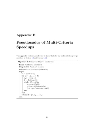
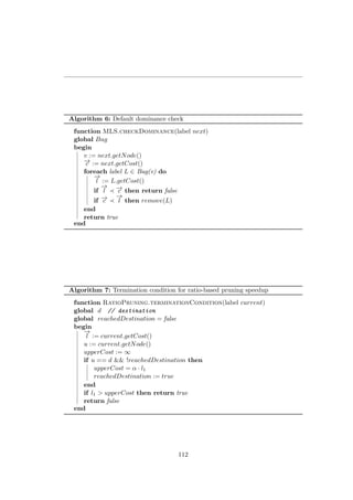


This doctoral thesis by Jan Hrnčíř from the Czech Technical University in Prague focuses on developing models and algorithms for sustainable journey planning. It addresses the problems of multi-criteria bicycle routing, intermodal journey planning across different transport modes, and ridesharing on timetabled public transport services. The thesis presents formal definitions of the problems, designs efficient algorithms to solve them, evaluates the algorithms using real-world data, and integrates the solutions into prototype journey planning systems that are validated through field trials with thousands of users. Finally, it discusses key aspects of engineering real-world journey planning systems.