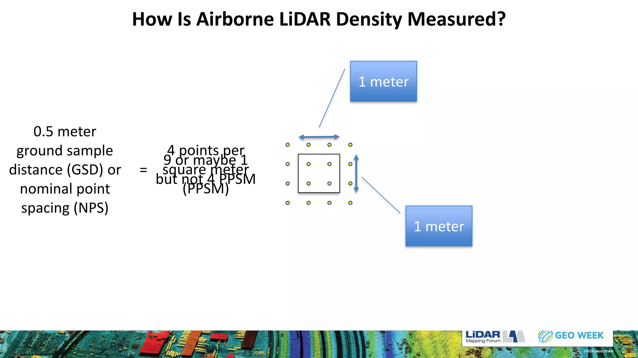
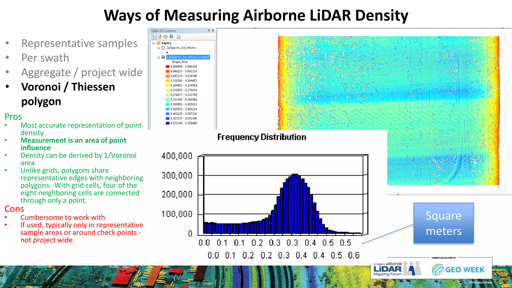
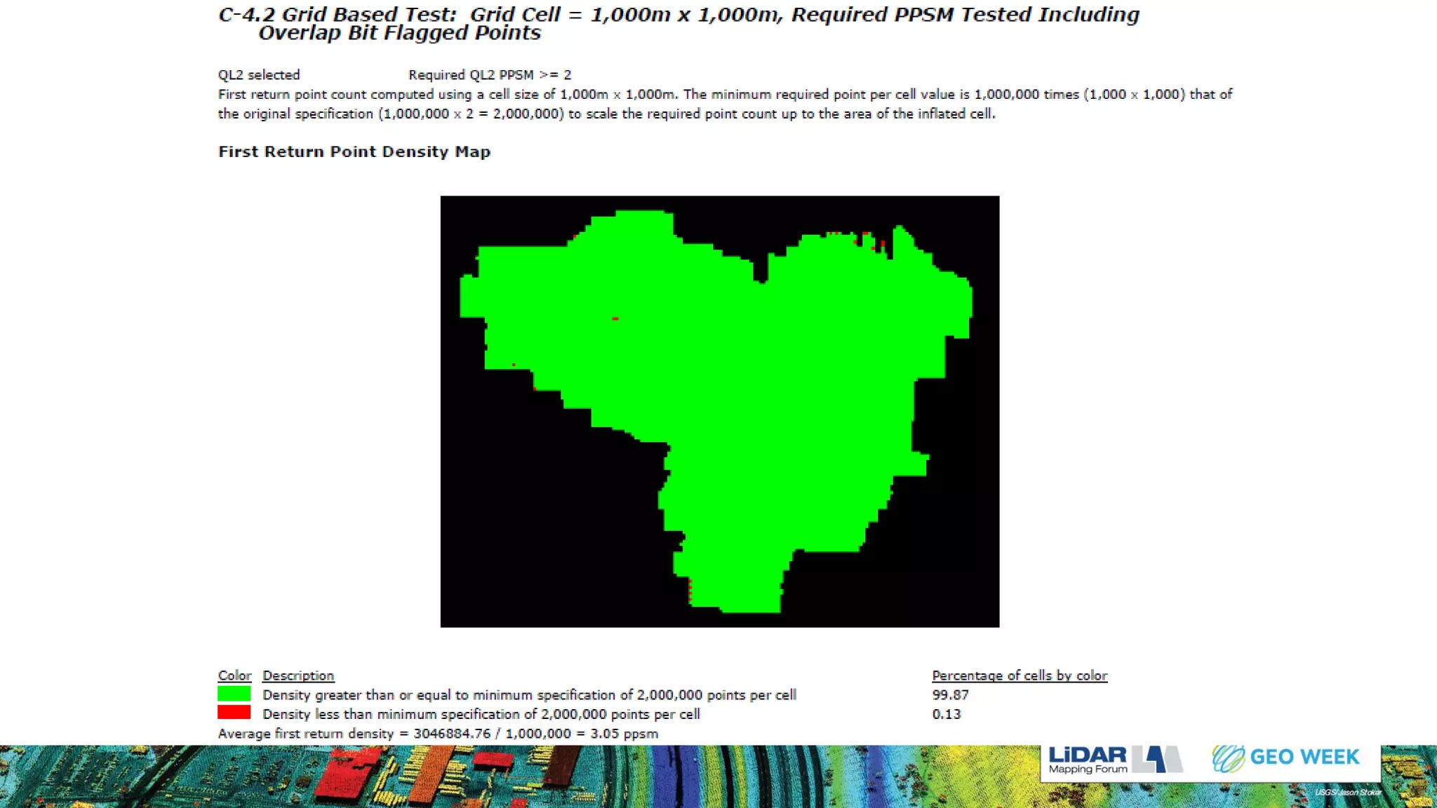
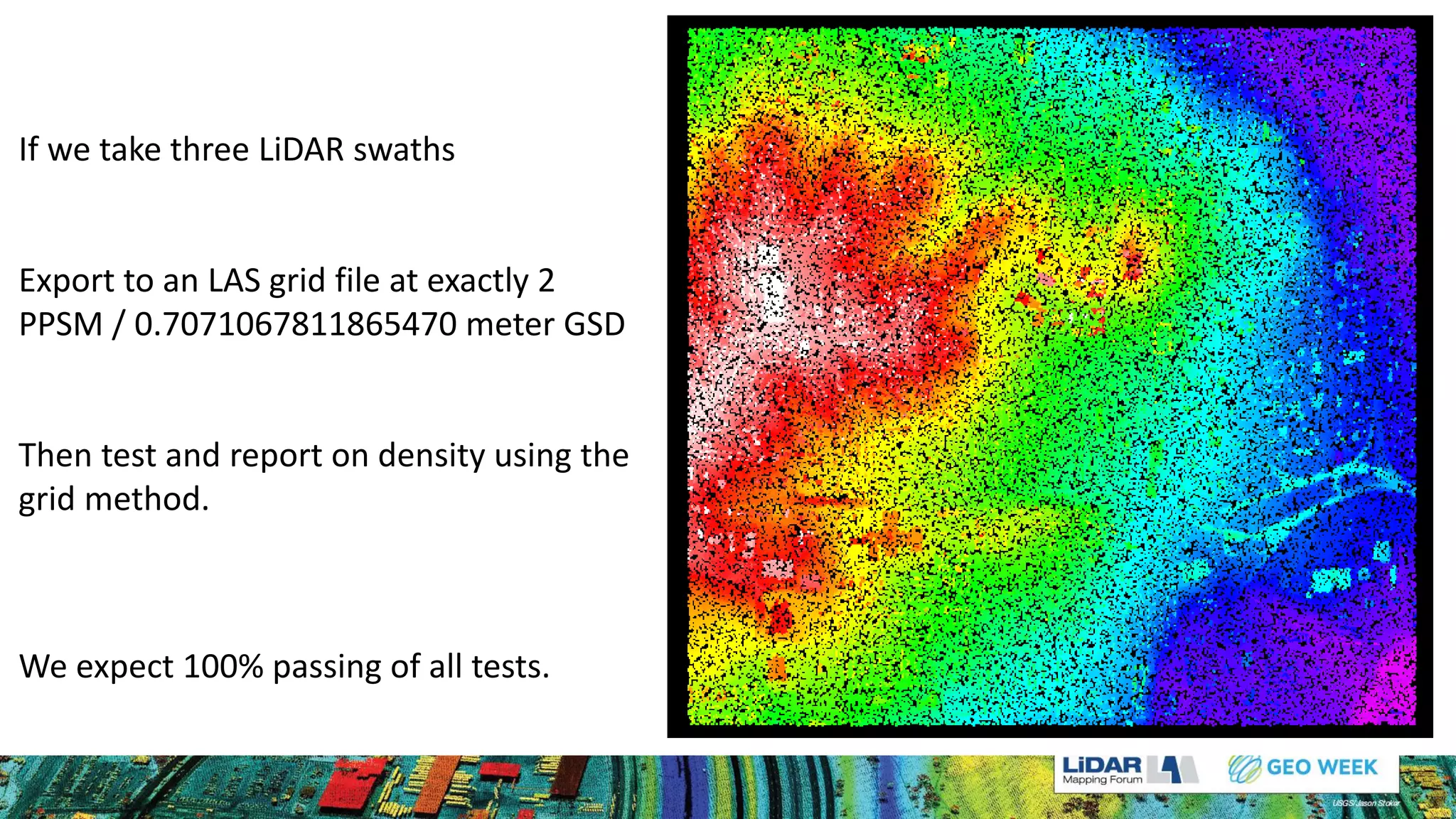
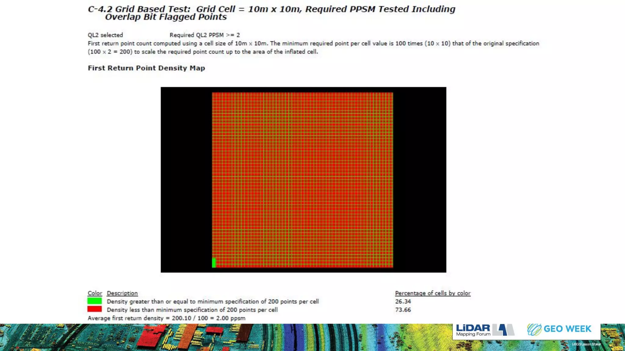
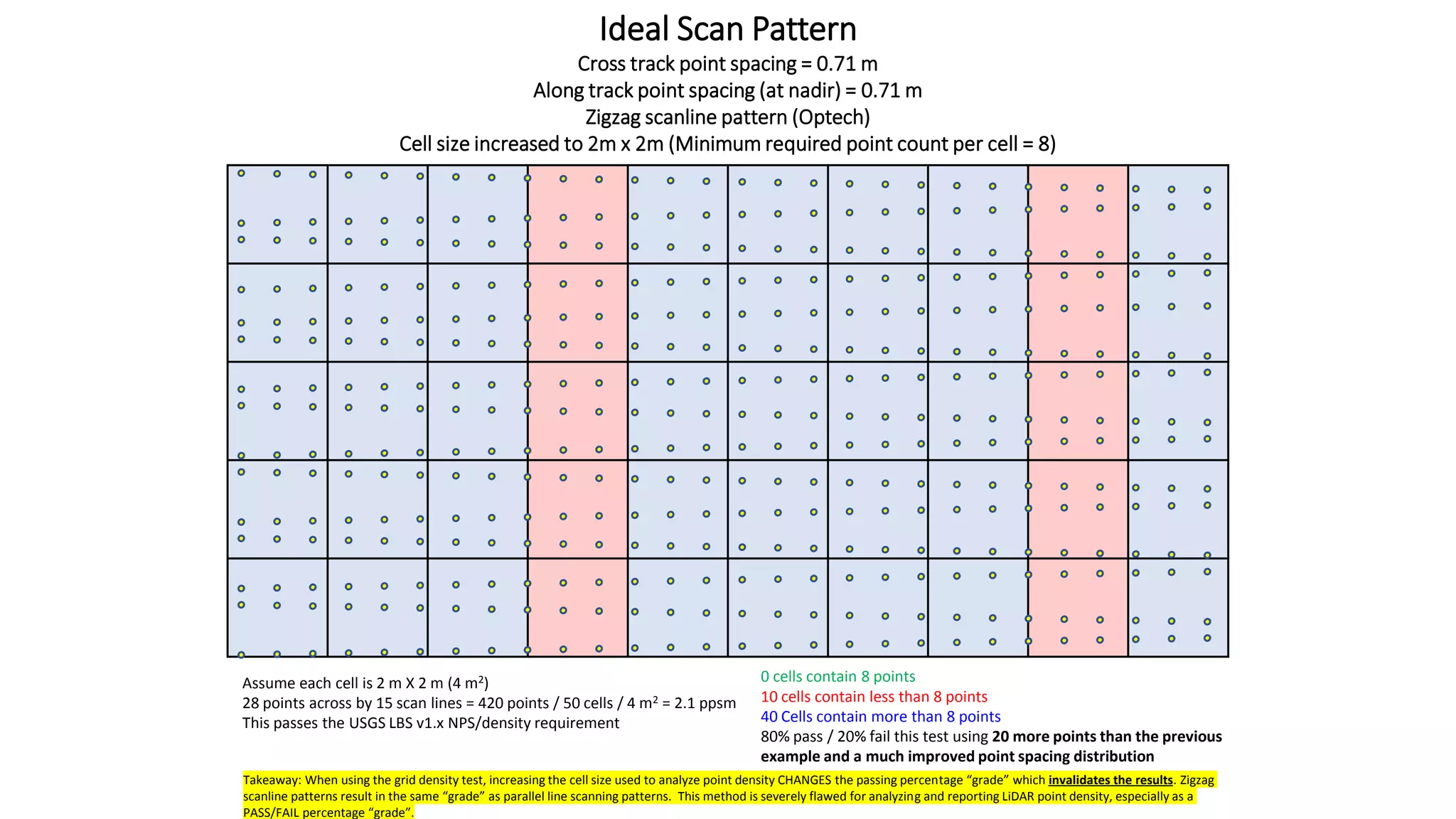
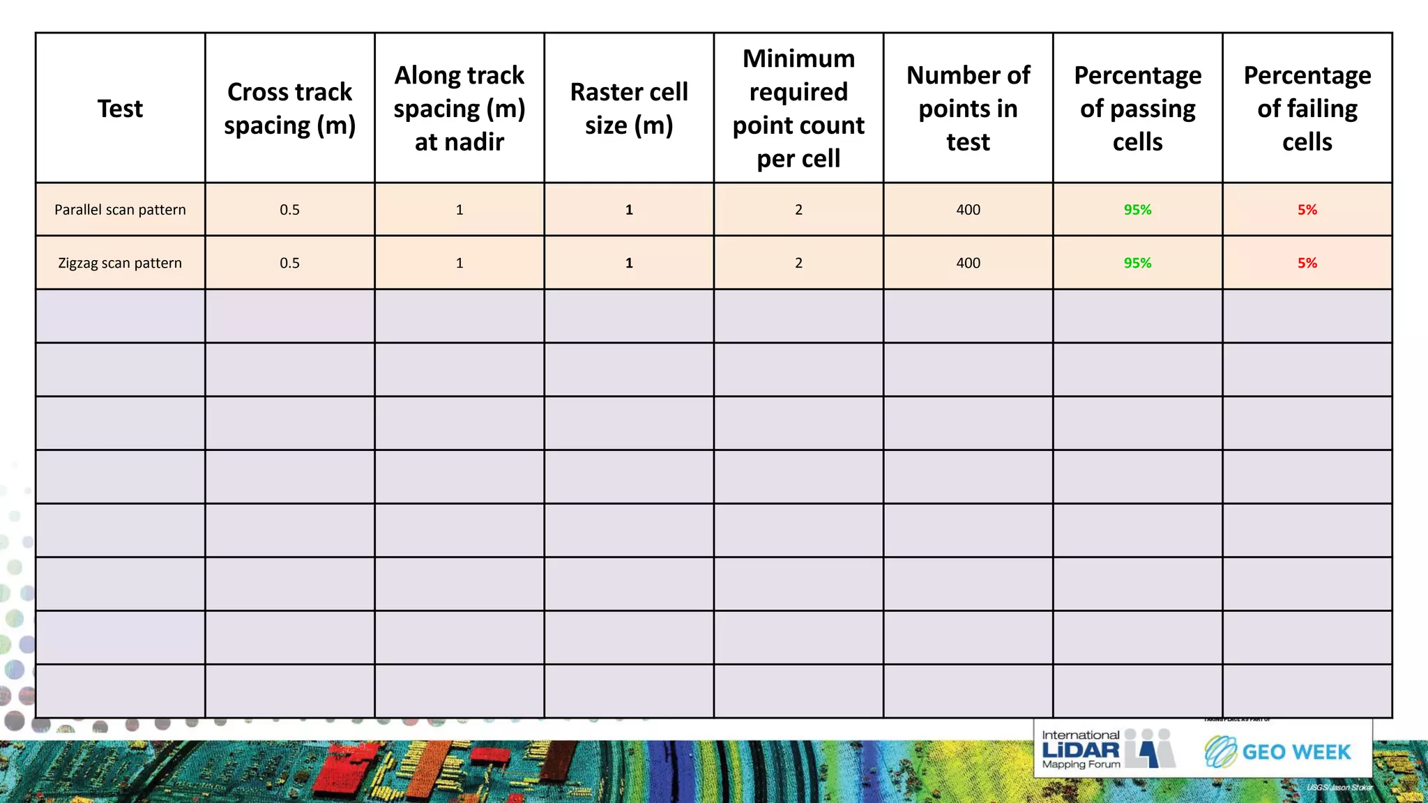
How is airborne LiDAR point density measured? How is it reported? What constitutes point density acceptance? The varied answers may surprise you. LiDAR providers, data QC entities, and end users go about this many different ways. It is eye opening to learn how open ended this topic is and how data density can be masked to look good but actually be compromised and vice versa. So what method is best? Maybe the answer depends on the application. This presentation will address these topics and uncover how a simple concept can be much more complicated than one would ever think. A better understanding of LiDAR point density is needed so that everyone involved can have clear measurement and reporting expectations at the beginning of projects.
Differential Global Positioning System (DGPS) is an enhancement to Global Positioning System that provides improved location accuracy, from the
15-meter nominal GPS accuracy to about 10 cm in case of the best implementations. Differential Global Positioning System (DGPS) is a method of providing differential corrections to a Global Positioning System (GPS) receiver in order to improve the accuracy of the navigation solution. DGPS corrections originate from a reference station at a known location. The receivers in these reference stations can estimate errors in the GPS because, unlike the general population of GPS receivers, they have an accurate knowledge of their position.
DGPS uses a network of fixed, ground-based reference stations to broadcast the difference between the positions indicated by the GPS (satellite) systems and the known fixed positions. These stations broadcast the difference between the measured satellite pseudoranges and actual (internally computed) pseudoranges, and receiver stations may correct their pseudoranges by the same amount. The digital correction signal is typically broadcast locally over ground-based transmitters of shorter range.
Unmanned Aerial Systems for Precision MappingUAS Colorado
Presentation by Renee Walmsley, Remote Sensing Program Manager at Tetra Tech, for the August 16, 2017 Rocky Mountain UAS Professionals Meetup at the Esri Broomfield office.
An Introduction to Laser Scanning - Part 3: Mobile mapping and accuracy chall...3D Laser Mapping
What is 3D mobile laser mapping and how does it work? What considerations need to be made when looking at the accuracy of a mobile mapping system?
This presentation talks about mobile mapping systems and accuracy. If the accuracy of the data you want to capture is important to you, what do you need to look out for or ask about?
If you would like more information about mobile mapping systems please get in touch - info@3dlasermapping.com or go to our website www.3dlasermapping.com/streetmapper
This content presents for basic of Synthetic Aperture Radar (SAR) including its geometry, how the image is created, essential parameters, interpretation, SAR sensor specification, and advantages and disadvantages.
LIDAR is an acronym for LIght Detection And Ranging. It is an optical remote sensing technology that can measure the distance to or other properties of a target by illuminating the target with light pulse to form an image.
This presentation will give a simple overview of image classification technique using difference type software focusing on object-based image classification and segmentation.
How to better understand SAR, interpret SAR products and realize the limitationsNopphawanTamkuan
This content shows how to better understand SAR (how to interpret SAR images and read SAR interferogram ). Moreover, capacities and limitations of SAR are discussed for each disaster emergency mapping (Flood, Landslide and Earthquake).
SBAS-DInSAR processing on the ESA Geohazards Exploitation PlatformEmmanuel Mathot
In the context of space-borne geodetic techniques, Differential Synthetic Aperture Radar Interferometry (DInSAR) has demonstrated its high performance in measuring surface displacements in different conditions and scenarios, both natural and anthropic. In particular, the advanced DInSAR time series processing method referred to as Small BAseline Subset (SBAS), that allows studying both the spatial and temporal variability of the surface displacements, has proven to be particularly suitable in different contexts, as for natural hazards (volcanoes, earthquakes and landslides) and human-induced deformation (subsidence due to aquifer exploitation, mining operations, and building of large infrastructures). Recently, an efficient implementation of this algorithm (referred to as P-SBAS approach) has been fully integrated within the ESA’s Grid Processing on Demand (G-POD) environment, which is part of the [Geohazards Thematic Exploitation Platform (GEP)](https://geohazards-tep.eo.esa.int/#!) of ESA. The GEP is devoted to the exploitation of EO data resources in the context of the Geohazard Supersites & Natural Laboratories as well as on the CEOS Pilots on Seismic Hazards and Volcanoes. The GEP is sourced with elements, data and processing, including P-SBAS, relevant to the geohazards theme. The integration of the P-SBAS algorithm within GEP resulted in a web-based tool freely available to the scientific community. This tool allows users to process, from their own laptops, the European SAR data archives (ERS, ENVISAT and Sentinel-1) for obtaining surface displacement maps and time series in a completely unsupervised way, without caring about data download and processing facility procurements. The workshop is organized in four parts. First, a short overview on the DInSAR processing methods allowing retrieving mean surface deformation maps and displacement time series will be provided, with a specific focus on the SBAS-DInSAR technique. Secondly, the GEP and G-POD environments will be introduced and the P-SBAS web tool will be presented. The third and the fourth parts are dedicated to the advanced features and to case studies and results achieved via the web tool, respectively.
Here is a corporate overview of Spectrum and some of our latest products. It includes our SDR-4000 SDR Radio modem, our RF-4902 rugged, frequency agile RF tuner, our SDR-2010 server-based signal processing platform, and our line of 3u VPX signal processing modems.
An Introduction to Laser Scanning - Part 2: Airborne LiDAR, the basics of tra...3D Laser Mapping
What type of scanners do Airborne laser scanning systems use? How do they work and why? This presentation covers the basics of Airborne Laser Scanning and some important things to consider if looking at this technology.
If you would like more information on this technology or you are looking for a system yourself? Please get in touch - www.3dlasermapping.com / info@3dlasermapping.com
An in depth examination of airborne lidar density measurement and reporting. This will review issues with existing methodologies and comparisons to a proposed replacement.
ASPRS LiDAR Division Update with a focus on quantifying horizontal sampling d...MattBethel1
This presentation will provide an update on the Lidar Division's work to produce an ASPRS document providing valuable information on airborne lidar density measuring and reporting.
This presentation will provide an update on the Lidar Division's work to produce an ASPRS document providing valuable information on airborne lidar density measuring and reporting. The scope of this document is:
• To clarify various definitions of density and related terms
• To document various methods for quantifying density
• To develop and document various methods for representation of density
• To document various tradeoffs among the methods of representation and quantification of density
• To provide recommendations on the use of density
Non-Uniform Random Feature Selection and Kernel Density Scoring With SVM Base...Sathishkumar Samiappan
Traditional statistical classification approaches often
fail to yield adequate results with Hyperspectral imagery (HSI) because
of the high dimensional nature of the data, multimodal class
distribution and limited ground truth samples for training. Over
the last decade, Support VectorMachines (SVMs) andMulti-Classifier
Systems (MCS) have become popular tools for HSI analysis.
Random Feature Selection (RFS) forMCS is a popular approach to
produce higher classification accuracies. In this study, we present a
Non-Uniform Random Feature Selection (NU-RFS) within a MCS
framework using SVMas the base classifier.We propose a method
to fuse the output of individual classifiers using scores derived from
kernel density estimation. This study demonstrates the improvement
in classification accuracies by comparing the proposed approach
to conventional analysis algorithms and by assessing the
sensitivity of the proposed approach to the number of training samples.
These results are compared with that of uniform RFS and regular
SVM classifiers. We demonstrate the superiority of Non-Uniform
based RFS system with respect to overall accuracy, user accuracies,
producer accuracies and sensitivity to number of training
samples.
This paper applies inverse transform sampling to sample training points for surrogate models. Inverse transform sampling uniformly generates a sequence of real numbers ranging from 0 to 1 as the probabilities at sample points. The coordinates of the sample points are evaluated using the inverse functions of Cumulative Distribution Functions (CDF). The inputs to surrogate models are assumed to be independent random variables. The sample points obtained by inverse transform sampling can effectively represent the frequency of occurrence of the inputs. The distributions of inputs to the surrogate models are fitted to their observed data. These distributions are used for inverse transform sampling. The sample points have larger densities in the regions where the Probability Density Functions (PDF) are higher. This sampling approach ensures that the regions with higher densities of sample points are more prevalent in the observations of the random variables. Inverse transform sampling is applied to the development of surrogate models for window performance evaluation. The distributions of the following three climatic conditions are fitted: (i) the outside temperature, (ii) the wind speed, and (iii) the solar radiation. The sample climatic conditions obtained by the inverse transform sampling are used as training points to evaluate the heat transfer through a generic triple pane window. Using the simulation results at the sample points, surrogate models are developed to represent the heat transfer through the window as a function of the climatic conditions. It is observed that surrogate models developed using the inverse transform sampling can provide higher accuracy than that developed using the Sobol sequence directly for the window performance evaluation.
Measurement Procedures for Design and Enforcement of Harm Claim ThresholdsPierre de Vries
Presentation at DySPAN 2017, March 2017
Paper forthcoming on IEEE Xplore
Paper authors:
Janne Riihijärvi, Petri Mähönen (RWTH Aachen University, Germany)
J. Pierre de Vries (Silicon Flatirons Centre, University of Colorado, USA)
Presentation of a research plan to use complex adaptive systems approaches to exploring the problem of optimizing geographical search in a wide variety of networks. Created to accompany a research proposal for EECS 594, Introduction to Adaptive Systems, at the University of Michigan.
Presented at #H2OWorld 2017 in Mountain View, CA.
Enjoy the video: https://youtu.be/bas3-Ue2qxc.
Learn more about H2O.ai: https://www.h2o.ai/.
Follow @h2oai: https://twitter.com/h2oai.
- - -
Abstract:
Auto Visualization involves the problem of producing meaningful graphics when presented with data. Relevant to this task are the strategies that expert statisticians and data analysts use to gain insights through visualization, as well as the portfolio of diagnostic methods devised by statisticians in the last 50 years. While some researchers and companies may claim to do automatic visualization, the problem is much deeper than simply producing collections of histograms, bar charts, and scatterplots. The deeper problem is what subset of these graphics is critical to recognizing anomalies, outliers, unusual distributions, missing values, and so on. This talk will cover aspects of this deeper problem and will introduce H2O software that implements some of these algorithms.
Leland Wilkinson is Chief Scientist at H2O.ai and Adjunct Professor of Computer Science at the University of Illinois Chicago. He received an A.B. degree from Harvard in 1966, an S.T.B. degree from Harvard Divinity School in 1969, and a Ph.D. from Yale in 1975. Wilkinson wrote the SYSTAT statistical package and founded SYSTAT Inc. in 1984. After the company grew to 50 employees, he sold SYSTAT to SPSS in 1994 and worked there for ten years on research and development of visualization systems. Wilkinson subsequently worked at Skytree and Tableau before joining H2O.ai. Wilkinson is a Fellow of the American Statistical Association, an elected member of the International Statistical Institute, and a Fellow of the American Association for the Advancement of Science. He has won best speaker award at the National Computer Graphics Association and the Youden prize for best expository paper in the statistics journal Technometrics. He has served on the Committee on Applied and Theoretical Statistics of the National Research Council and is a member of the Boards of the National Institute of Statistical Sciences (NISS) and the Institute for Pure and Applied Mathematics (IPAM). In addition to authoring journal articles, the original SYSTAT computer program and manuals, and patents in visualization and distributed analytic computing, Wilkinson is the author (with Grant Blank and Chris Gruber) of Desktop Data Analysis with SYSTAT. He is also the author of The Grammar of Graphics, the foundation for several commercial and opensource visualization systems (IBMRAVE, Tableau, Rggplot2, and PythonBokeh).
Approximation models (or surrogate models) provide an efficient substitute to expen- sive physical simulations and an efficient solution to the lack of physical models of system behavior. However, it is challenging to quantify the accuracy and reliability of such ap- proximation models in a region of interest or the overall domain without additional system evaluations. Standard error measures, such as the mean squared error, the cross-validation error, and the Akaikes information criterion, provide limited (often inadequate) informa- tion regarding the accuracy of the final surrogate. This paper introduces a novel and model independent concept to quantify the level of errors in the function value estimated by the final surrogate in any given region of the design domain. This method is called the Re- gional Error Estimation of Surrogate (REES). Assuming the full set of available sample points to be fixed, intermediate surrogates are iteratively constructed over a sample set comprising all samples outside the region of interest and heuristic subsets of samples inside the region of interest (i.e., intermediate training points). The intermediate surrogate is tested over the remaining sample points inside the region of interest (i.e., intermediate test points). The fraction of sample points inside region of interest, which are used as interme- diate training points, is fixed at each iteration, with the total number of iterations being pre-specified. The estimated median and maximum relative errors within the region of in- terest for the heuristic subsets at each iteration are used to fit a distribution of the median and maximum error, respectively. The estimated statistical mode of the median and the maximum error, and the absolute maximum error are then represented as functions of the density of intermediate training points, using regression models. The regression models are then used to predict the expected median and maximum regional errors when all the sample points are used as training points. Standard test functions and a wind farm power generation problem are used to illustrate the effectiveness and the utility of such a regional error quantification method.
International Journal of Engineering Research and Applications (IJERA) is an open access online peer reviewed international journal that publishes research and review articles in the fields of Computer Science, Neural Networks, Electrical Engineering, Software Engineering, Information Technology, Mechanical Engineering, Chemical Engineering, Plastic Engineering, Food Technology, Textile Engineering, Nano Technology & science, Power Electronics, Electronics & Communication Engineering, Computational mathematics, Image processing, Civil Engineering, Structural Engineering, Environmental Engineering, VLSI Testing & Low Power VLSI Design etc.
This presentation by Morris Kleiner (University of Minnesota), was made during the discussion “Competition and Regulation in Professions and Occupations” held at the Working Party No. 2 on Competition and Regulation on 10 June 2024. More papers and presentations on the topic can be found out at oe.cd/crps.
This presentation was uploaded with the author’s consent.
Acorn Recovery: Restore IT infra within minutesIP ServerOne
Introducing Acorn Recovery as a Service, a simple, fast, and secure managed disaster recovery (DRaaS) by IP ServerOne. A DR solution that helps restore your IT infra within minutes.
0x01 - Newton's Third Law: Static vs. Dynamic AbusersOWASP Beja
f you offer a service on the web, odds are that someone will abuse it. Be it an API, a SaaS, a PaaS, or even a static website, someone somewhere will try to figure out a way to use it to their own needs. In this talk we'll compare measures that are effective against static attackers and how to battle a dynamic attacker who adapts to your counter-measures.
About the Speaker
===============
Diogo Sousa, Engineering Manager @ Canonical
An opinionated individual with an interest in cryptography and its intersection with secure software development.
Sharpen existing tools or get a new toolbox? Contemporary cluster initiatives...Orkestra
UIIN Conference, Madrid, 27-29 May 2024
James Wilson, Orkestra and Deusto Business School
Emily Wise, Lund University
Madeline Smith, The Glasgow School of Art
Have you ever wondered how search works while visiting an e-commerce site, internal website, or searching through other types of online resources? Look no further than this informative session on the ways that taxonomies help end-users navigate the internet! Hear from taxonomists and other information professionals who have first-hand experience creating and working with taxonomies that aid in navigation, search, and discovery across a range of disciplines.
Obesity causes and management and associated medical conditions
AIRBORNE LIDAR POINT DENSITY
1. AIRBORNE LIDAR POINT DENSITY, MORE TO THE POINT
July 23, 2019
Matt Bethel
Director of Operations and Technology
Merrick & Company
2. How Is Airborne LiDAR Density Measured?
0.5
meter
0.5
meter
0.5 meter
ground sample
distance (GSD) or
nominal point
spacing (NPS)
3. How Is Airborne LiDAR Density Measured?
Type equation here.
1 meter
1 meter
4 points per
square meter
(PPSM)
=
𝐍𝐏𝐒 =
𝟏
𝑫𝒆𝒏𝒔𝒊𝒕𝒚
𝑫𝒆𝒏𝒔𝒊𝒕𝒚 =
𝟏
𝑵𝑷𝑺 𝟐0.5 meter
ground sample
distance (GSD) or
nominal point
spacing (NPS)
𝑫𝒆𝒏𝒔𝒊𝒕𝒚 =
𝐟𝐢𝐫𝐬𝐭 𝐨𝐫 𝐥𝐚𝐬𝐭 𝐫𝐞𝐭𝐮𝐫𝐧 𝐩𝐨𝐢𝐧𝐭 𝐜𝐨𝐮𝐧𝐭
𝒂𝒓𝒆𝒂
4. How Is Airborne LiDAR Density Measured?
1 meter
1 meter
9 or maybe 1
but not 4 PPSM
=
4 points per
square meter
(PPSM)
0.5 meter
ground sample
distance (GSD) or
nominal point
spacing (NPS)
5. How Is Airborne LiDAR Density Measured?
confusing=
Q: Are points on cell
boundaries shared for density
calculations?
A: No, they must be counted
within only one cell.
REMEMBER
THIS!!!
0.5 meter
ground sample
distance (GSD) or
nominal point
spacing (NPS)
6. Ways of Measuring Airborne LiDAR Density
• Representative samples
Pros
• Fast and easy to calculate
• Good for areas of interests
Cons
• Biased by many factors such
as sidelap, patches,
turbulence, etc.
• Very localized, not
representative of swaths or
project extents
• Cannot automatedly find
problem areas that could be
considered failures /
specification violations
• Difficult to use for reporting
7. Ways of Measuring Airborne LiDAR Density
• Representative samples
• Per swath
Pros
• Ideal to compare against
planned swath density
• Relatively easy to compute
• Reasonably batchable – one
process per flightline
• Good to use for reporting
• Is not biased (inflated) by sidelap
• No hidden problems with use or
reporting – very straightforward
Cons
• Needs interpretation if flying
>50% sidelap to achieve planned
density
8. Ways of Measuring Airborne LiDAR Density
• Representative samples
• Per swath
• Aggregate / project
wide
Pros
• Considers all collected points
• Good for reporting
• Straightforward approach
(number of first or last return
points / area of project boundary)
Cons
• Crosslines, sidelap, collection
block overlap, and patches can
inflate density results
• Tabular reporting only will not
identify localized density failures.
A thematic raster is needed for
locating localized density failures.
Area of Project Boundary (m2)
9. Ways of Measuring Airborne LiDAR Density
• Representative samples
• Per swath
• Aggregate / project wide
• Voronoi / Thiessen
polygon
Pros
• Most accurate representation of point
density
• Measurement is an area of point
influence
• Density can be derived by 1/Voronoi
area
• Unlike grids, polygons share
representative edges with neighboring
polygons. With grid cells, four of the
eight neighboring cells are connected
through only a point.
Cons
• Cumbersome to work with
• If used, typically only in representative
sample areas or around check points -
not project wide
10. Ways of Measuring Airborne LiDAR Density
• Representative samples
• Per swath
• Aggregate / project wide
• Voronoi / Thiessen
polygon
Square
meters
Pros
• Most accurate representation of point
density
• Measurement is an area of point
influence
• Density can be derived by 1/Voronoi
area
• Unlike grids, polygons share
representative edges with neighboring
polygons. With grid cells, four of the
eight neighboring cells are connected
through only a point.
Cons
• Cumbersome to work with
• If used, typically only in representative
sample areas or around check points -
not project wide
11. Ways of Measuring Airborne LiDAR Density
• Representative samples
• Per swath
• Aggregate / project wide
• Voronoi / Thiessen
polygon
PPSM
Pros
• Most accurate representation of point
density
• Measurement is an area of point
influence
• Density can be derived by 1/Voronoi
area
• Unlike grids, polygons share
representative edges with neighboring
polygons. With grid cells, four of the
eight neighboring cells are connected
through only a point.
Cons
• Cumbersome to work with
• If used, typically only in representative
sample areas or around check points -
not project wide
12. Ways of Measuring Airborne LiDAR Density
• Representative samples
• Per swath
• Aggregate / project wide
• Voronoi / Thiessen
polygon
• Grid / raster / tile
Pros
• Fast and easy to calculate
• Seemingly straightforward approach – use grid or tile scheme to count
points and report on lowest divisible points per grid/tile area
• Easy to use for reporting – pass fail percentage results and graphic
Cons
• The results are in pass/fail cell counts yet there are no establish
parameters for use or analysis (no passing thresholds)
• User selected processing cell size changes the results
• Inherent with major problems
• Results are severely misunderstood yet widely used and relied upon
13.
14.
15.
16.
17. There is a better way…
• In digital signal processing, the minimum sampling rate is limited to 2X the
maximum frequency. The purpose for this limit is to preserve important
information throughout the transformation. This is known as the Nyquist-
Shannon sampling theorem. This 2X law can be applied to LiDAR density
measurement and derivative grid creation. This is known as the Nyquist
sampling criteria.
• The Nyquist sampling criteria states that we must sample at no less than twice
the resolution of the smallest detail we intend to measure or model.
• This means that grids used for density calculation or raster product creation
must have a cell size no less than 2 x NPS.
18.
19.
20.
21. Third Party Reports Showing
Varying Pass/Fail Percentage Results
These first return density reports were generated using third party software ran on two sample swaths using
different cell sizes (highlighted in each screenshot). Note the percentages widely vary with each cell size test.
22. That was all real LiDAR data with
random point spacing.
Let’s test synthetically created,
perfectly spaced point data.
23. If we take three LiDAR swaths
Export to an LAS grid file at exactly 2
PPSM / 0.7071067811865470 GSD
Then test and report on density using the
grid method.
We expect 100% passing of all tests.
24. If we take three LiDAR swaths
Export to an LAS grid file at exactly 2
PPSM / 0.7071067811865470 meter GSD
Then test and report on density using the
grid method.
We expect 100% passing of all tests.
31. Less than Ideal Scan Pattern
Cross track point spacing = 0.5 m
Along track point spacing = 1 m
Parallel scanline pattern (Riegl)
(Minimum required point count per cell = 2)
190 cells contain 2 points
10 cells contain only 1 point
95% pass / 5% fail this test
Assume each cell is 1 m X 1 m (1 m2)
40 points across by 10 scan lines = 400 points / 200 cells = 2 ppsm
This passes the USGS LBS v1.x NPS/density requirement
Takeaway: Data with poor point spacing geometry can yield a high passing percentage “grade” using the grid
density test method.
32. Less than Ideal Scan Pattern
Cross track point spacing = 0.5 m
Along track point spacing = 1 m
Zigzag scanline pattern (Optech)
(Minimum required point count per cell = 2)
190 cells contain 2 points
10 cells contain only 1 point
95% pass / 5% fail this test
Assume each cell is 1 m X 1 m (1 m2)
40 points across by 10 scan lines = 400 points / 200 cells = 2 ppsm
This passes the USGS LBS v1.x NPS/density requirement
Takeaway: Data with poor point spacing geometry can yield a high passing percentage “grade” using the grid
density test method. Zigzag scanline patterns result in the same “grade” as parallel line scanning patterns.
33. Ideal Scan Pattern
Cross track point spacing = 0.71 m
Along track point spacing = 0.71 m
Parallel scanline pattern (Riegl)
(Minimum required point count per cell = 2)
100 cells contain 2 points
60 cells contain only 1 point
40 Cells contain more than 2 points
70% pass / 30% fail this test using 20 more points than the previous
example and a much improved point spacing distribution
Assume each cell is 1 m X 1 m (1 m2)
28 points across by 15 scan lines = 420 points / 200 cells = 2.1 ppsm
This passes the USGS LBS v1.x NPS/density requirement
Takeaway: Data with ideal point spacing geometry results in a much lower passing percentage “grade” using the grid density test method.
This method is severely flawed for analyzing and reporting LiDAR point density, especially as a PASS/FAIL percentage “grade”.
34. Ideal Scan Pattern
Cross track point spacing = 0.71 m
Along track point spacing (at nadir) = 0.71 m
Zigzag scanline pattern (Optech)
(Minimum required point count per cell = 2)
98 cells contain 2 points
60 cells contain only 1 point
42 Cells contain more than 2 points
70% pass / 30% fail this test using 20 more points than the previous
example and a much improved point spacing distribution
Assume each cell is 1 m X 1 m (1 m2)
28 points across by 15 scan lines = 420 points / 200 cells = 2.1 ppsm
This passes the USGS LBS v1.x NPS/density requirement
Takeaway: Data with ideal point spacing geometry results in a much lower passing percentage “grade” using the grid density test method. Zigzag scanline patterns result in the same “grade” as
parallel line scanning patterns. This method is severely flawed for analyzing and reporting LiDAR point density, especially as a PASS/FAIL percentage “grade”.
36. Ideal Scan Pattern
Cross track point spacing = 0.71 m
Along track point spacing = 0.71 m
Parallel scanline pattern (Riegl)
Cell size increased to 2m x 2m (Minimum required point count per cell = 8)
0 cells contain 8 points
10 cells contain less than 8 points
40 Cells contain more than 8 points
80% pass / 20% fail this test using 20 more points than the previous
example and a much improved point spacing distribution
Assume each cell is 2 m X 2 m (4 m2)
28 points across by 15 scan lines = 420 points / 50 cells / 4 m2 = 2.1 ppsm
This passes the USGS LBS v1.x NPS/density requirement
Takeaway: When using the grid density test, increasing the cell size used to analyze point density CHANGES the passing percentage “grade” which
invalidates the results. This method is severely flawed for analyzing and reporting LiDAR point density, especially as a PASS/FAIL percentage “grade”.
37. Ideal Scan Pattern
Cross track point spacing = 0.71 m
Along track point spacing (at nadir) = 0.71 m
Zigzag scanline pattern (Optech)
Cell size increased to 2m x 2m (Minimum required point count per cell = 8)
0 cells contain 8 points
10 cells contain less than 8 points
40 Cells contain more than 8 points
80% pass / 20% fail this test using 20 more points than the previous
example and a much improved point spacing distribution
Assume each cell is 2 m X 2 m (4 m2)
28 points across by 15 scan lines = 420 points / 50 cells / 4 m2 = 2.1 ppsm
This passes the USGS LBS v1.x NPS/density requirement
Takeaway: When using the grid density test, increasing the cell size used to analyze point density CHANGES the passing percentage “grade” which invalidates the results. Zigzag
scanline patterns result in the same “grade” as parallel line scanning patterns. This method is severely flawed for analyzing and reporting LiDAR point density, especially as a
PASS/FAIL percentage “grade”.
38. Ideal Scan Pattern
Cross track point spacing = 0.71 m
Along track point spacing = 0.71 m
Parallel scanline pattern (Riegl)
Cell size increased to 5m x 5m (Minimum required point count per cell = 50)
0 cells contain 50 points
4 cells contain less than 50 points
4 Cells contain more than 50 points
50% pass / 50% fail this test using 20 more points than the previous
example and a much improved point spacing distribution
Assume each cell is 5 m X 5 m (25 m2)
28 points across by 15 scan lines = 420 points / 8 cells / 25 m2 = 2.1 ppsm
This passes the USGS LBS v1.x NPS/density requirement
Takeaway: When using the grid density test, increasing the cell size used to analyze point density CHANGES the passing percentage “grade” which
invalidates the results. This method is severely flawed for analyzing and reporting LiDAR point density, especially as a PASS/FAIL percentage “grade”.
39. Ideal Scan Pattern
Cross track point spacing = 0.71 m
Along track point spacing (at nadir) = 0.71 m
Zigzag scanline pattern (Optech)
Cell size increased 5m x 5m (Minimum required point count per cell = 50)
0 cells contain 50 points
3 cells contain less than 50 points
5 Cells contain more than 50 points
60% pass / 40% fail this test using 20 more points than the previous
example and a much improved point spacing distribution
Assume each cell is 5 m X 5 m (25 m2)
28 points across by 15 scan lines = 420 points / 8 cells / 25 m2 = 2.1 ppsm
This passes the USGS LBS v1.x NPS/density requirement
Takeaway: When using the grid density test, increasing the cell size used to analyze point density CHANGES the passing percentage “grade” which invalidates the results.
Zigzag scanline patterns result in a similar “grade” as parallel line scanning patterns. This method is severely flawed for analyzing and reporting LiDAR point density, especially as
a PASS/FAIL percentage “grade”.
40. Ideal Scan Pattern With Nyquist Sampling Criteria
Cross track point spacing = 0.71 m
Along track point spacing = 0.71 m
Parallel scanline pattern (Riegl)
(Minimum required point count per cell = 1)
420 Cells contain more than 1 point
100% pass / 0% fail this test using
Assume each cell is 1.42m X 1.42 m (2.02 m2)
28 points across by 15 scan lines = 420 points / 200 cells = 2.1 ppsm
This passes the USGS LBS v1.x NPS/density requirement
Takeaway: Data with ideal point spacing geometry results in a 100% passing percentage “grade” using the Nyquist sampling criteria grid
density test method.
41. Ideal Scan Pattern With Nyquist Sampling Criteria
Cross track point spacing = 0.71 m
Along track point spacing (at nadir) = 0.71 m
Zigzag scanline pattern (Optech)
(Minimum required point count per cell = 1)
Takeaway: Data with ideal point spacing geometry results in a 100% passing percentage “grade” using the Nyquist sampling criteria grid density
test method. Zigzag scanline patterns result in the same “grade” as parallel line scanning patterns.
420 Cells contain more than 1 point
100% pass / 0% fail this test using
Assume each cell is 1.42m X 1.42 m (2.02 m2)
28 points across by 15 scan lines = 420 points / 200 cells = 2.1 ppsm
This passes the USGS LBS v1.x NPS/density requirement
42. Test
Cross track
spacing (m)
Along track
spacing (m)
at nadir
Raster cell
size (m)
Minimum
required
point count
per cell
Number of
points in
test
Percentage
of passing
cells
Percentage
of failing
cells
43. Test
Cross track
spacing (m)
Along track
spacing (m)
at nadir
Raster cell
size (m)
Minimum
required
point count
per cell
Number of
points in
test
Percentage
of passing
cells
Percentage
of failing
cells
Parallel scan pattern 0.5 1 1 2 400 95% 5%
Zigzag scan pattern 0.5 1 1 2 400 95% 5%
44. Test
Cross track
spacing (m)
Along track
spacing (m)
at nadir
Raster cell
size (m)
Minimum
required
point count
per cell
Number of
points in
test
Percentage
of passing
cells
Percentage
of failing
cells
Parallel scan pattern 0.5 1 1 2 400 95% 5%
Zigzag scan pattern 0.5 1 1 2 400 95% 5%
Parallel scan pattern 0.71 0.71 1 2 420 70% 30%
Zigzag scan pattern 0.71 0.71 1 2 420 70% 30%
45. Test
Cross track
spacing (m)
Along track
spacing (m)
at nadir
Raster cell
size (m)
Minimum
required
point count
per cell
Number of
points in
test
Percentage
of passing
cells
Percentage
of failing
cells
Parallel scan pattern 0.5 1 1 2 400 95% 5%
Zigzag scan pattern 0.5 1 1 2 400 95% 5%
Parallel scan pattern 0.71 0.71 1 2 420 70% 30%
Zigzag scan pattern 0.71 0.71 1 2 420 70% 30%
Parallel scan pattern 0.71 0.71 2 8 420 80% 20%
Zigzag scan pattern 0.71 0.71 2 8 420 80% 20%
46. Test
Cross track
spacing (m)
Along track
spacing (m)
at nadir
Raster cell
size (m)
Minimum
required
point count
per cell
Number of
points in
test
Percentage
of passing
cells
Percentage
of failing
cells
Parallel scan pattern 0.5 1 1 2 400 95% 5%
Zigzag scan pattern 0.5 1 1 2 400 95% 5%
Parallel scan pattern 0.71 0.71 1 2 420 70% 30%
Zigzag scan pattern 0.71 0.71 1 2 420 70% 30%
Parallel scan pattern 0.71 0.71 2 8 420 80% 20%
Zigzag scan pattern 0.71 0.71 2 8 420 80% 20%
Parallel scan pattern 0.71 0.71 5 50 420 50% 50%
Zigzag scan pattern 0.71 0.71 5 50 420 60% 40%
48. Conclusions and Recommendations
• Representative samples are too limiting for project analysis and reporting.
• Swath density analysis is straightforward, reliable, well understood, and very representative.
• Aggregate is too generalizing. A supplemental raster is required to identify localized failures.
• Voronoi is the most accurate but too cumbersome to use for thorough project analysis.
• Grid/raster/tile density method is very effective only if using the Nyquist sampling criteria. A
qualifying pass/fail threshold is required. Also, the results of this method are consistent with
the results from the reliable swath density analysis.
• Never use the flawed grid method with a simple points per square area calculation.
49. Thank You
Matt Bethel
Director of Operations and Technology
Merrick & Company
http://www.merrick.com/Geospatial
matt.bethel@merrick.com
(303) 353-3662