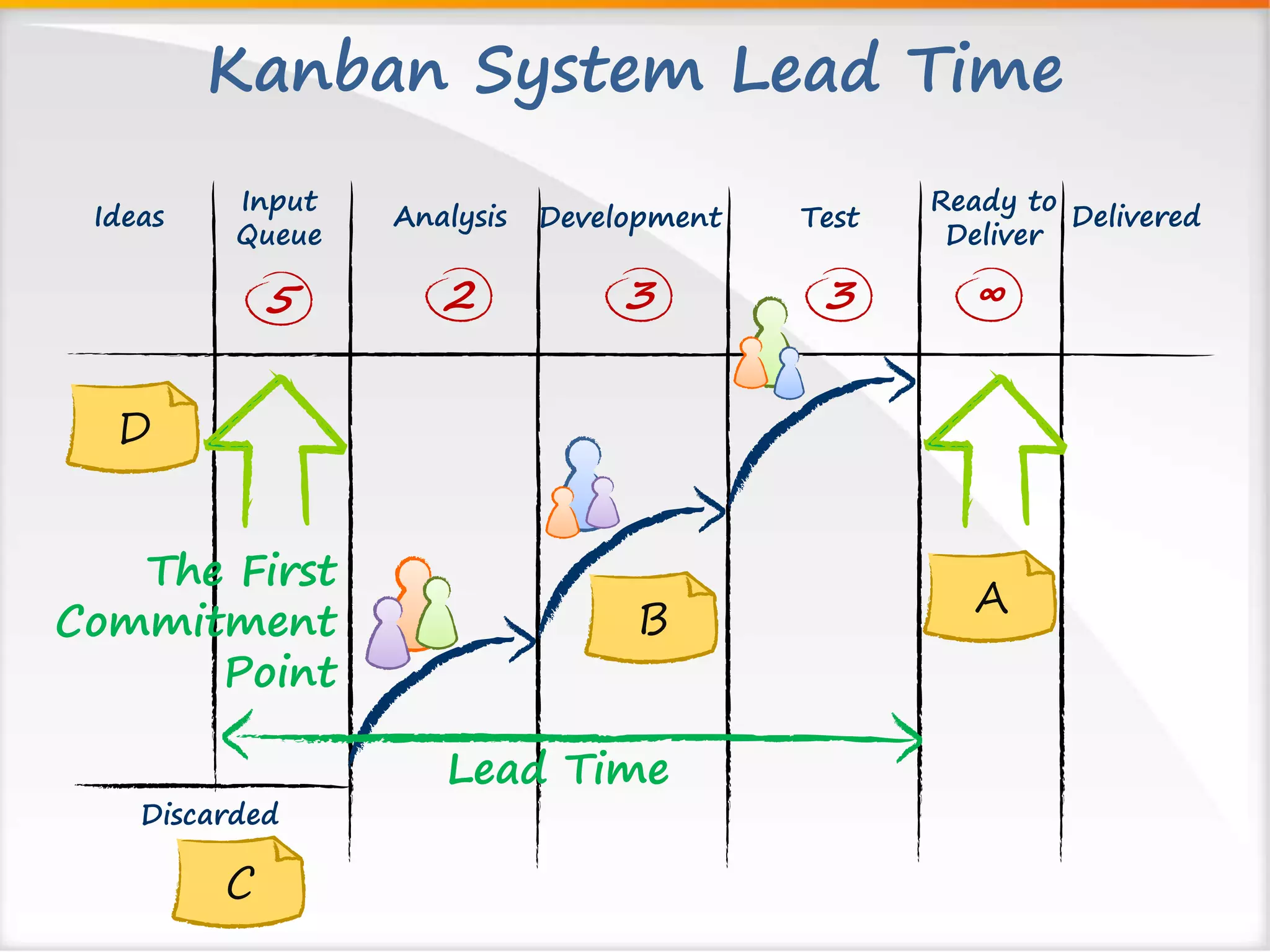
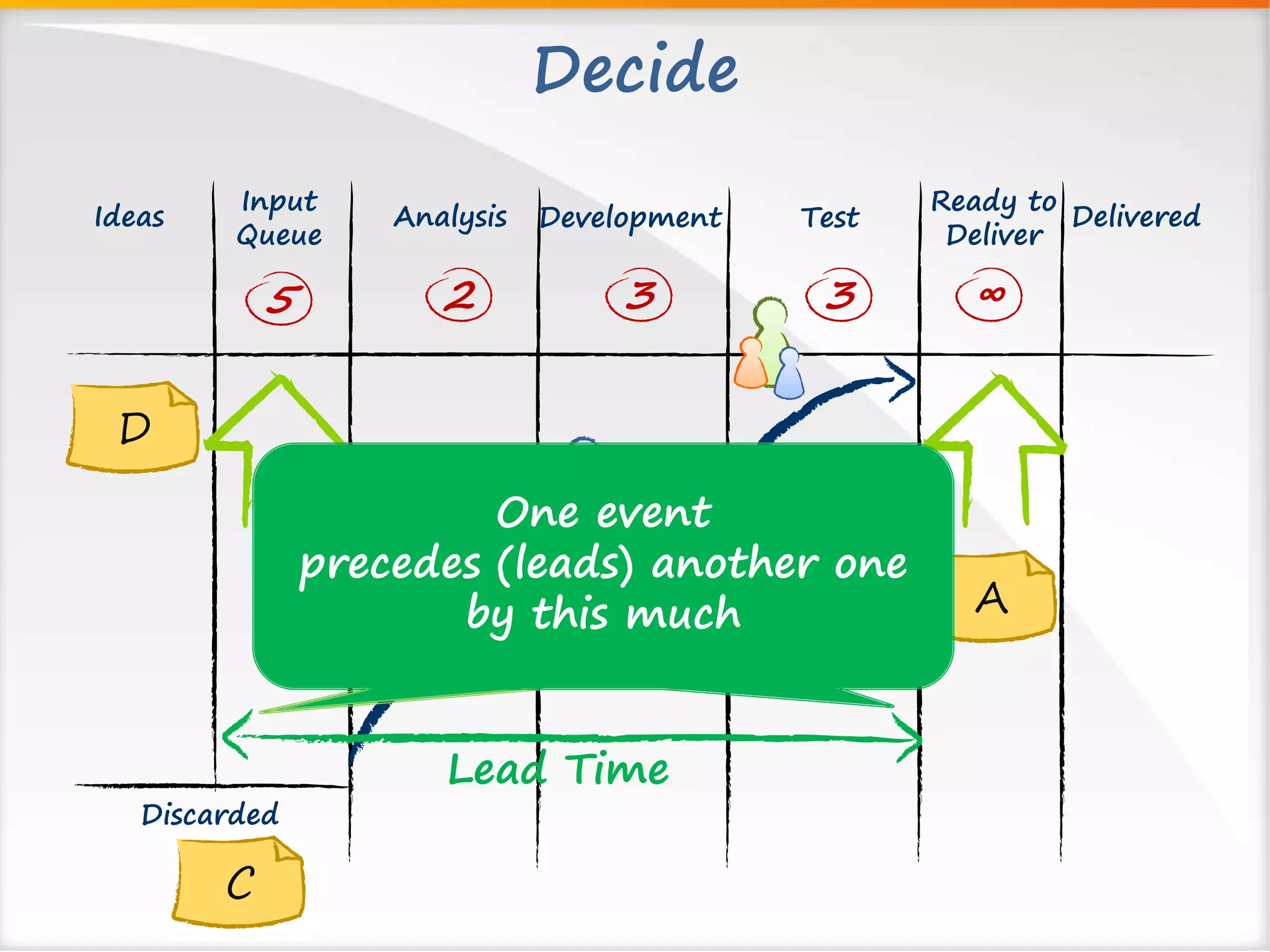
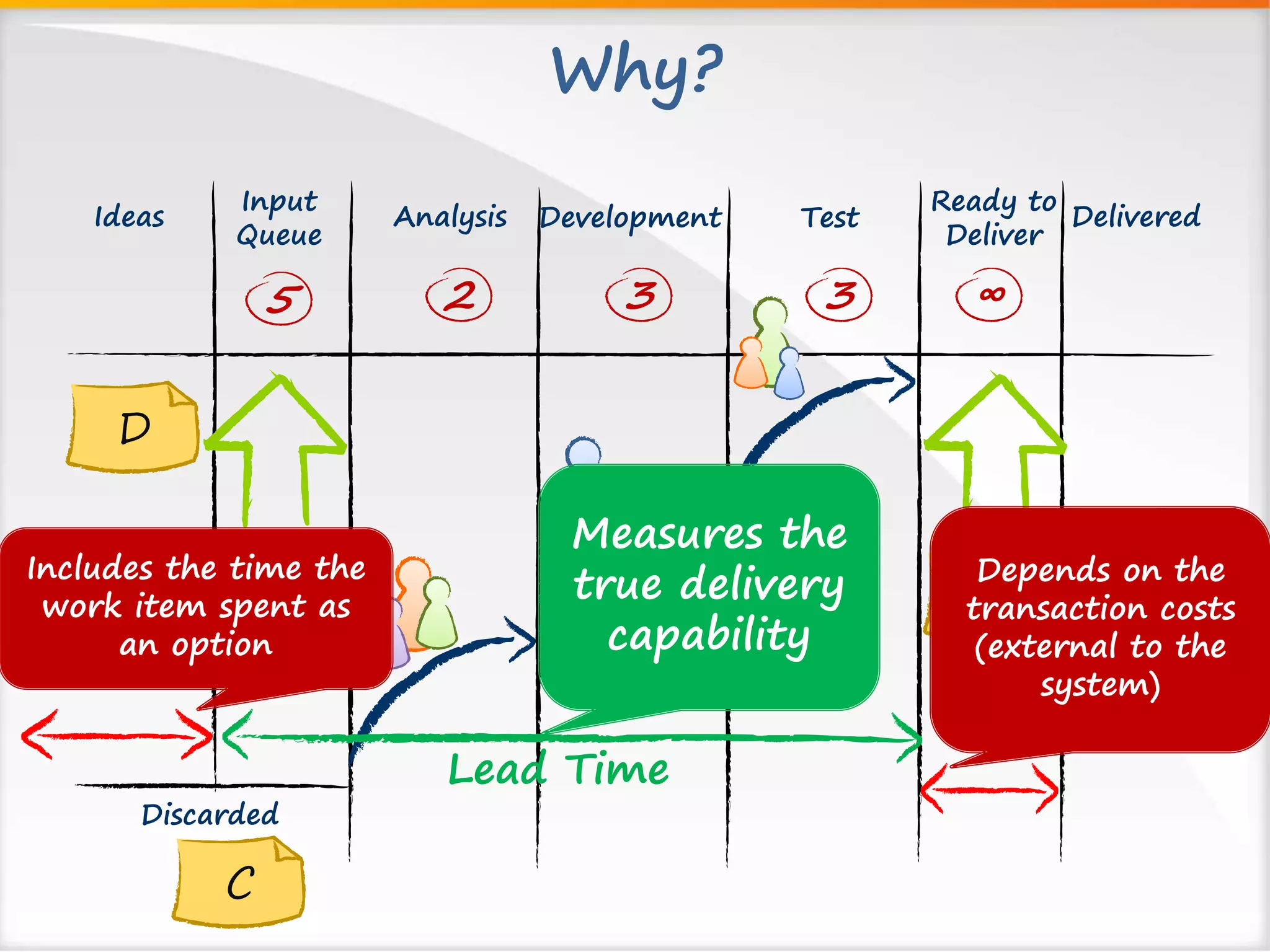
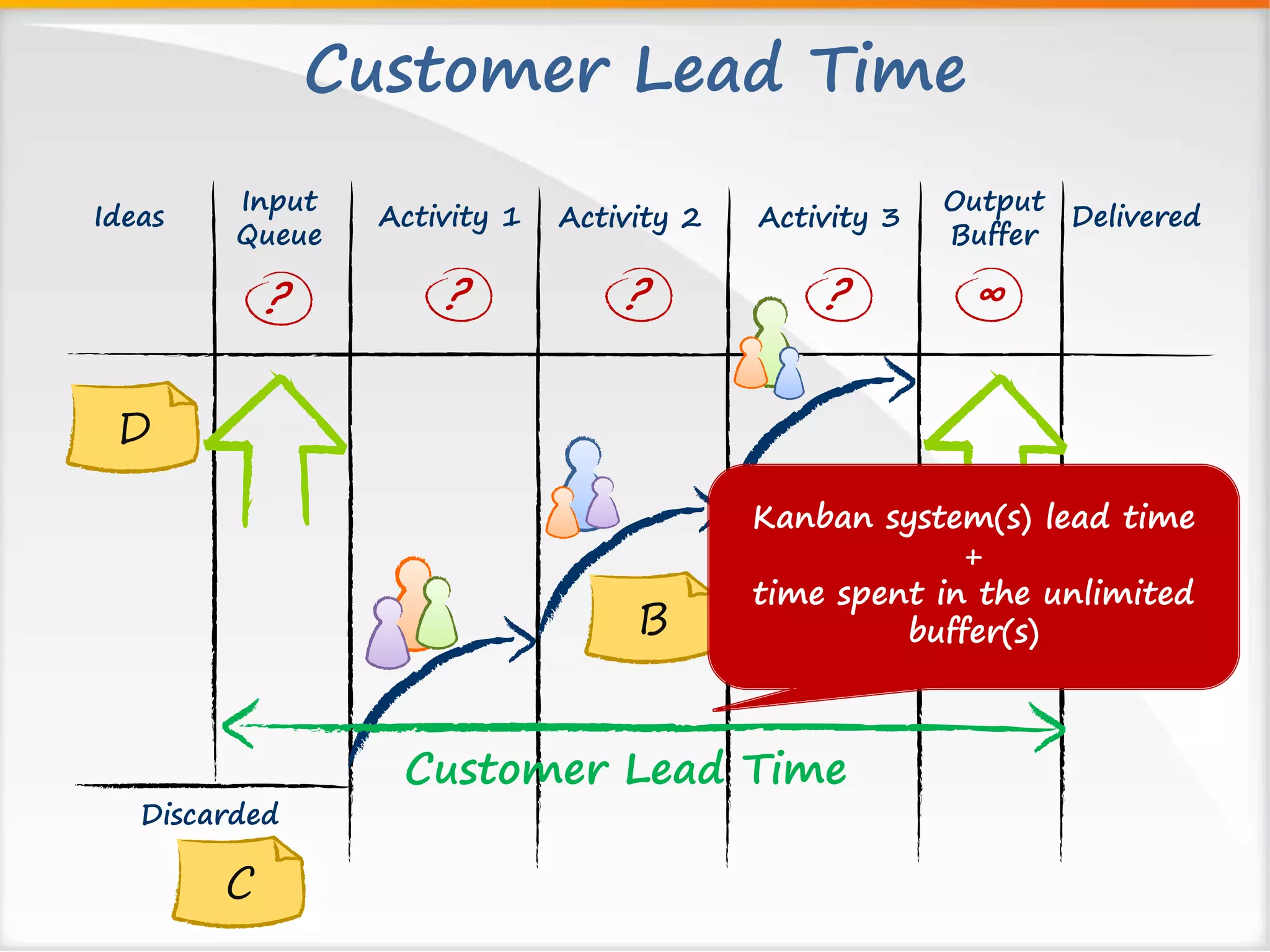
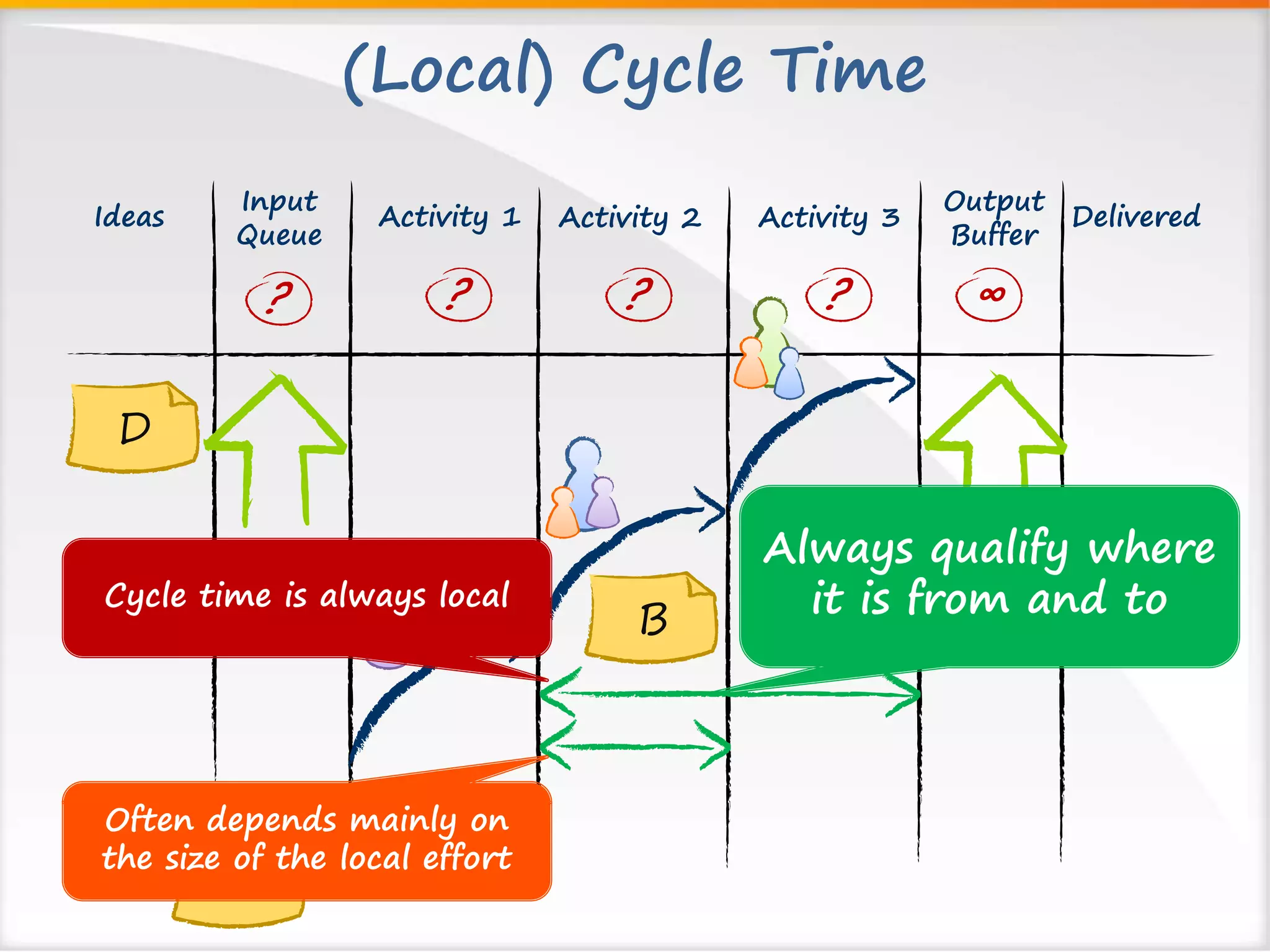
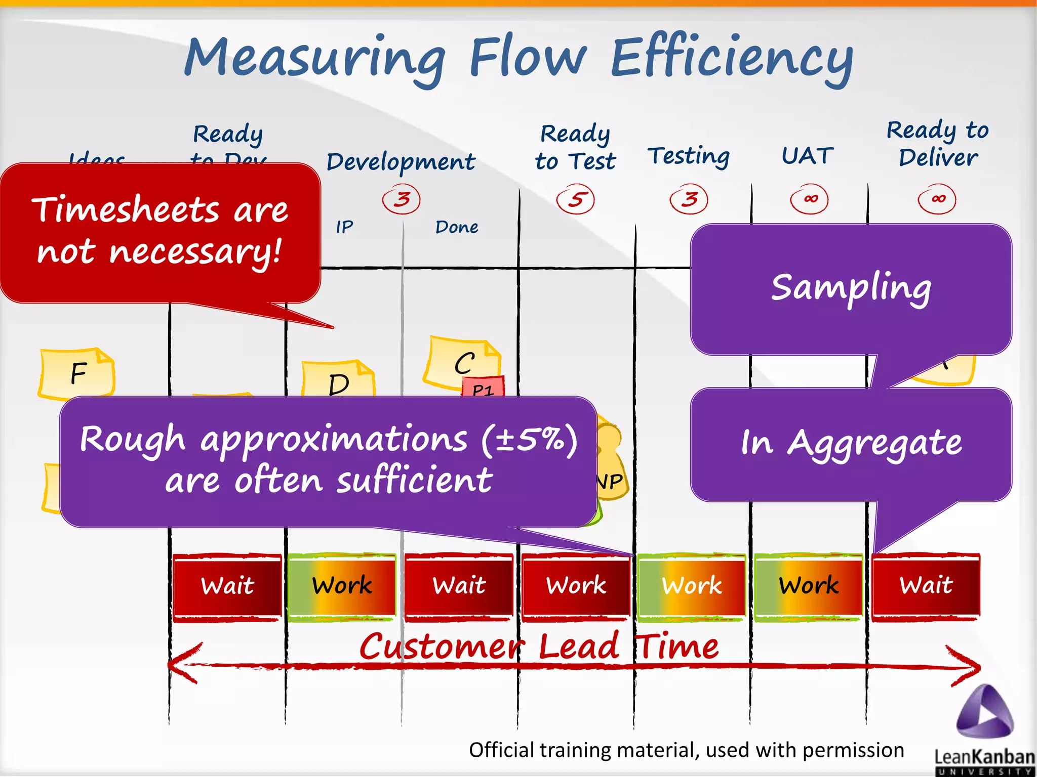
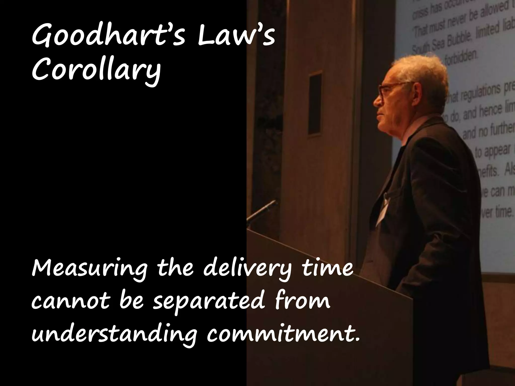
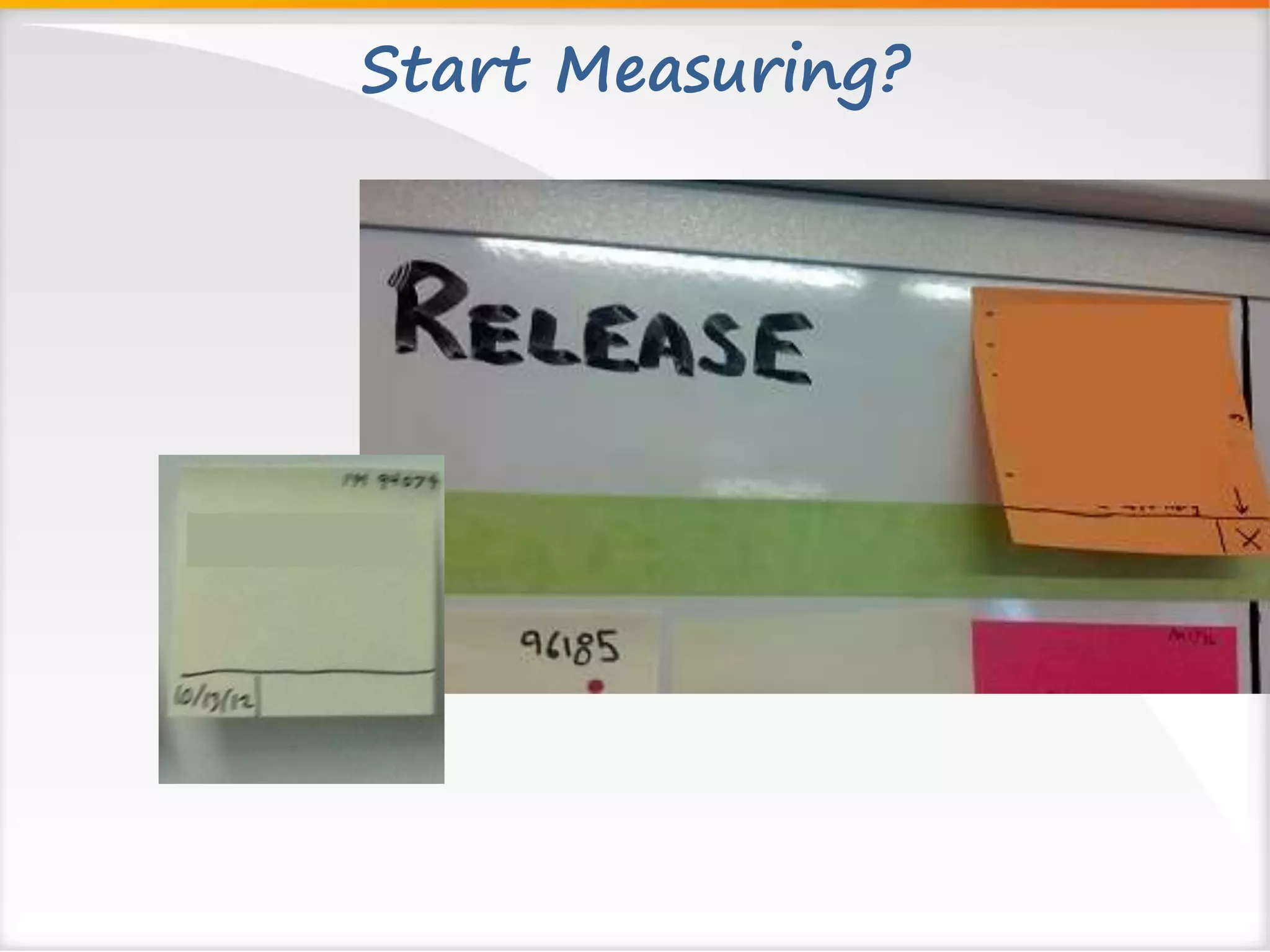
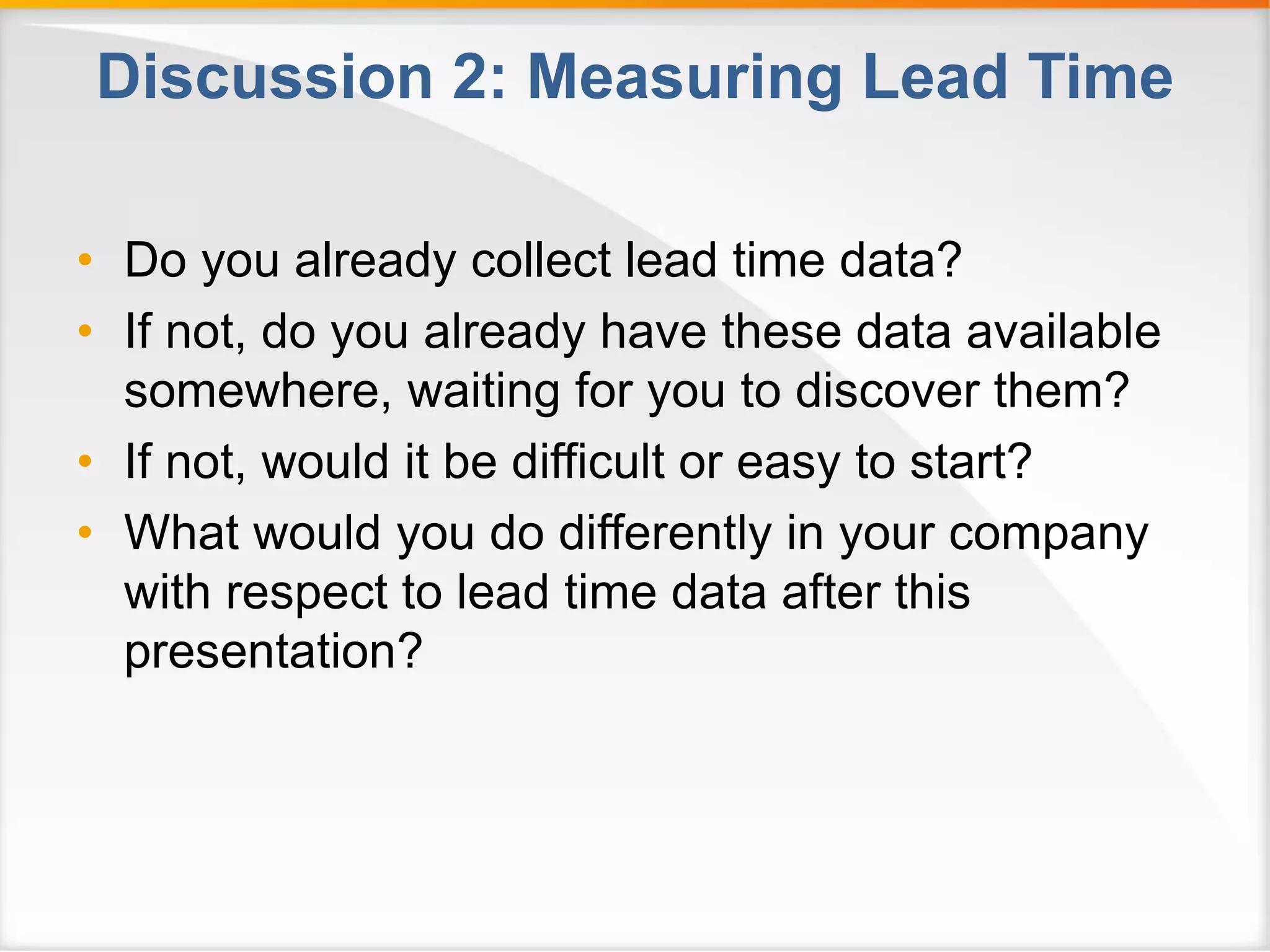
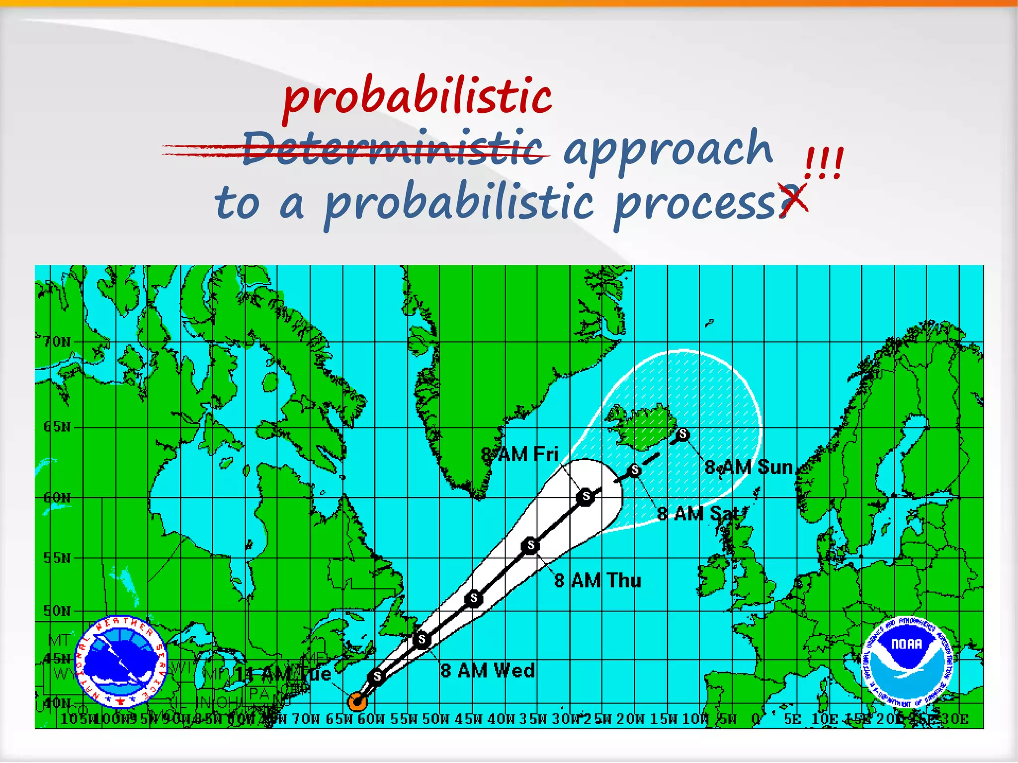
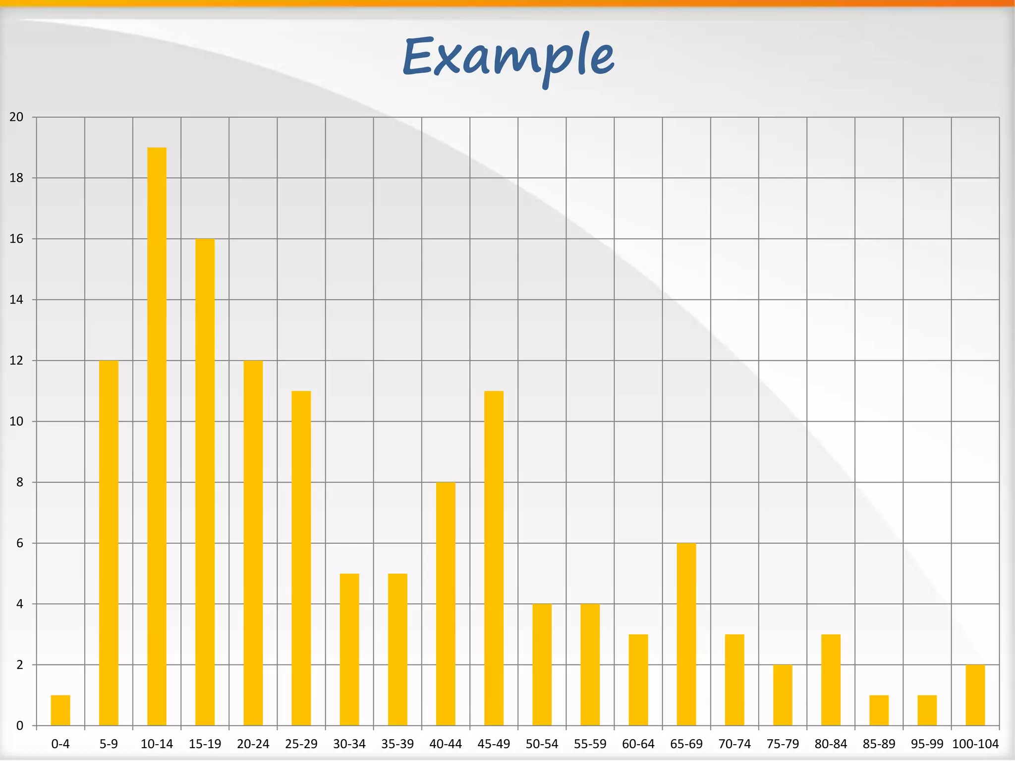
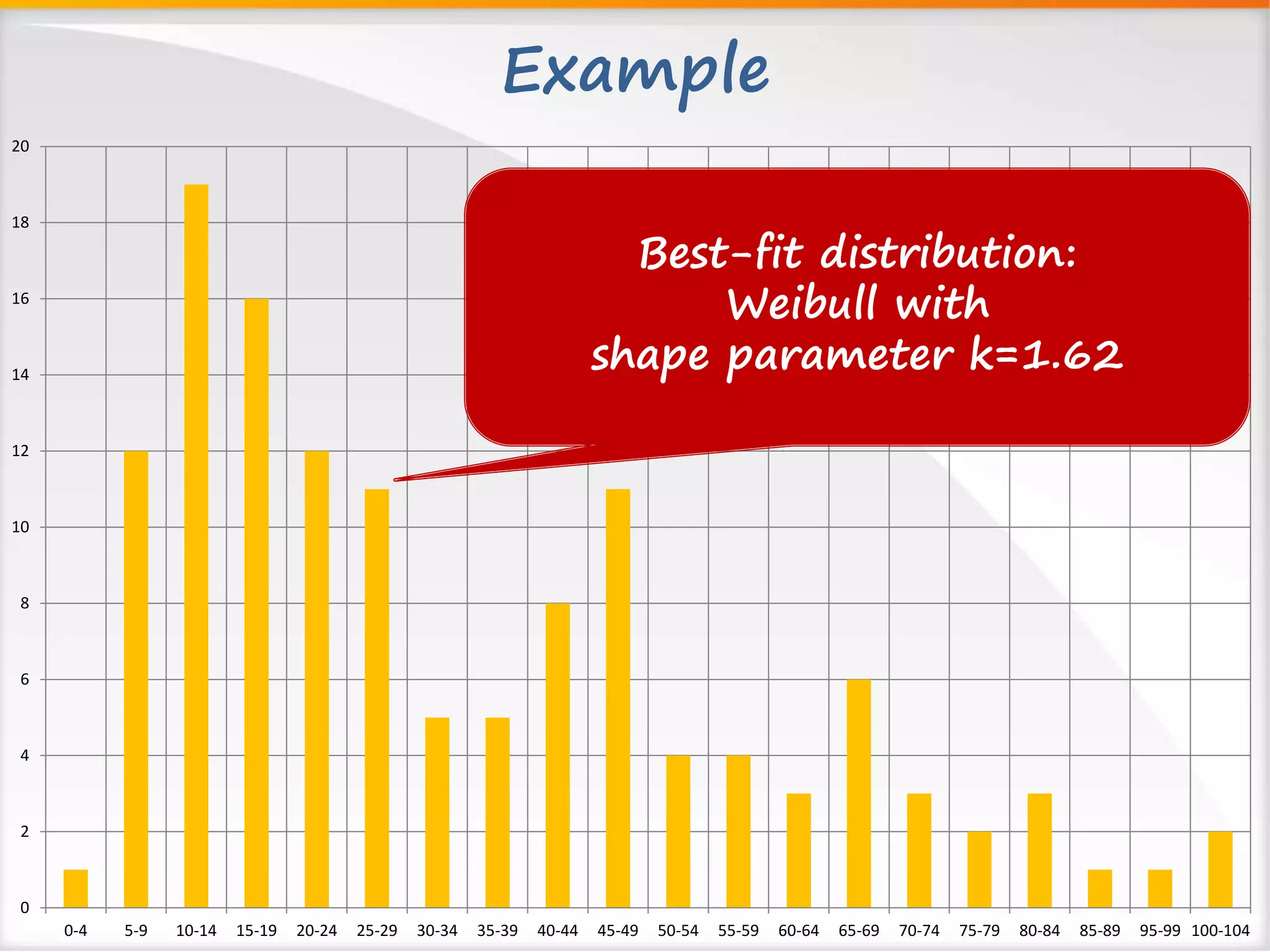
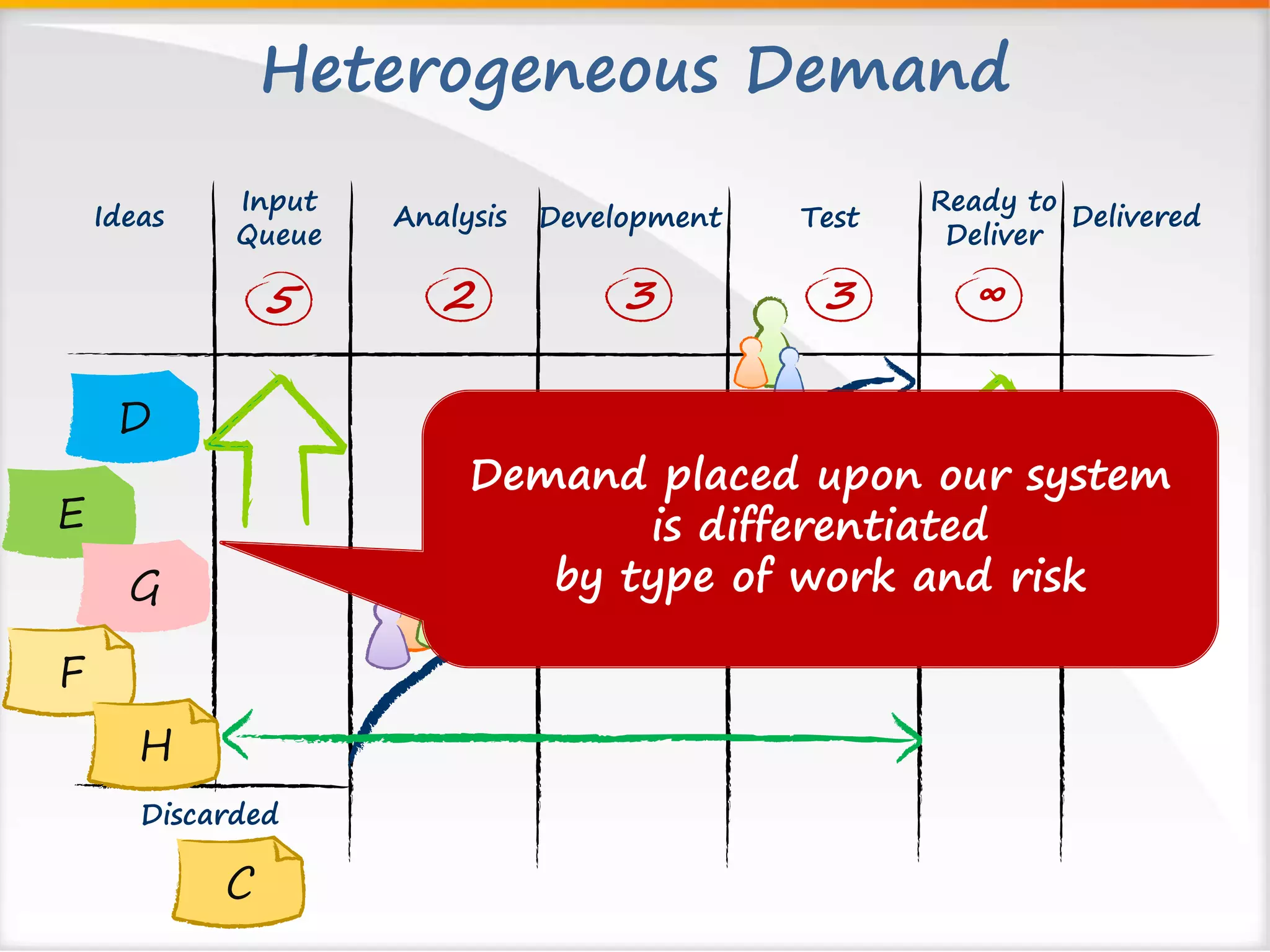
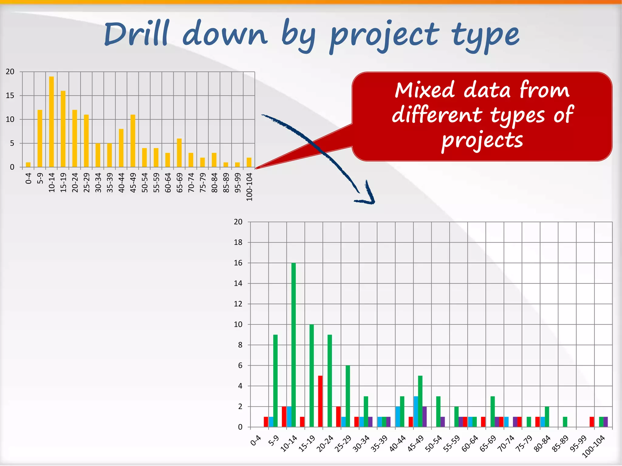
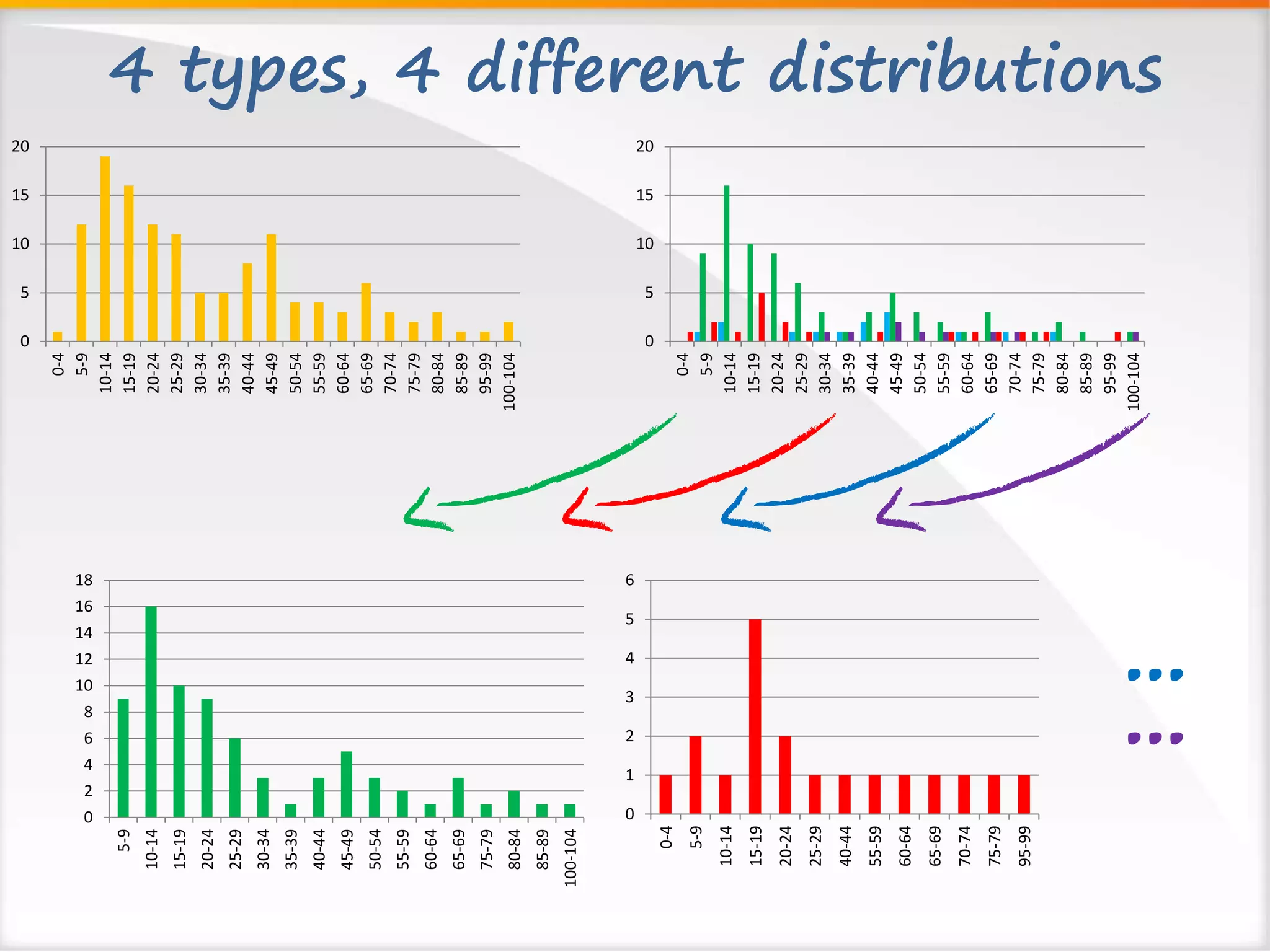
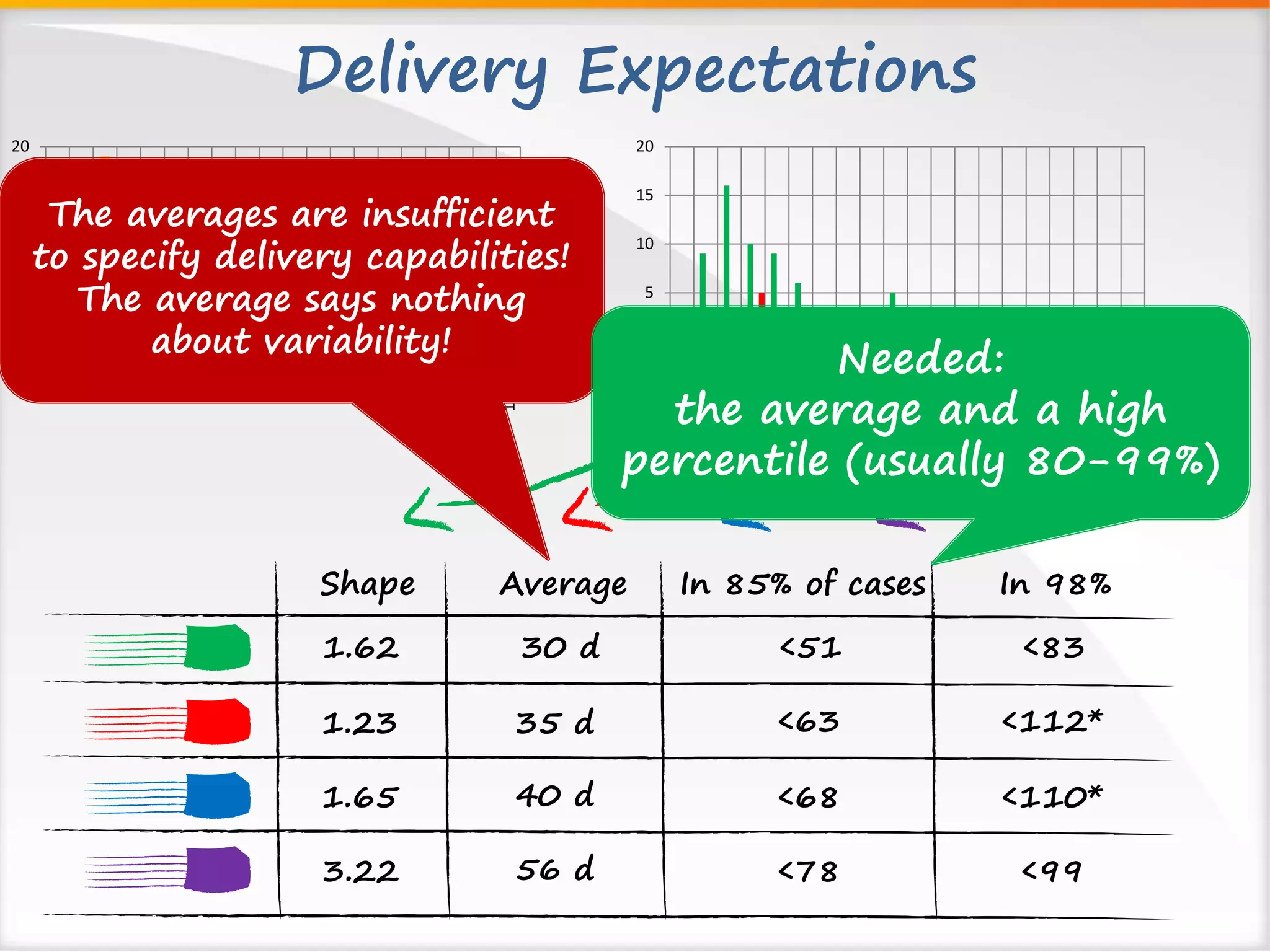
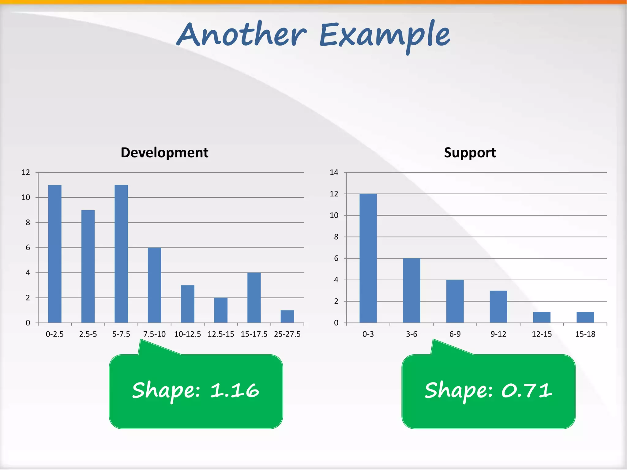
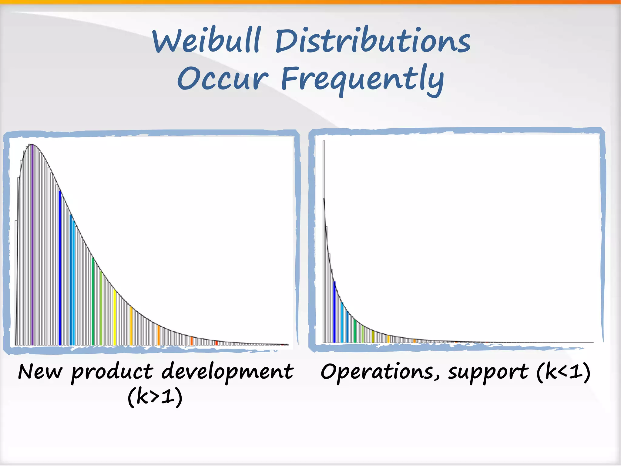
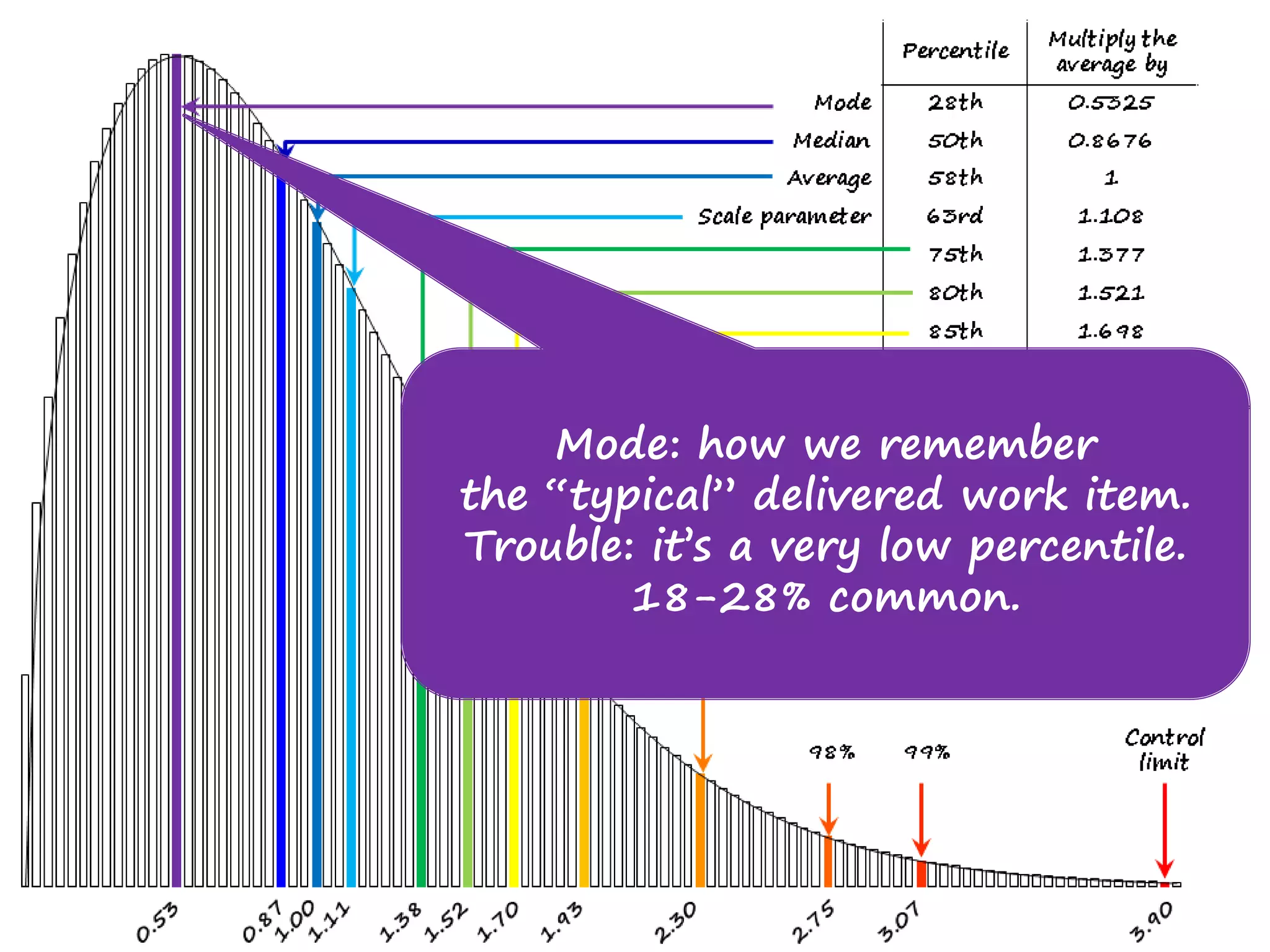
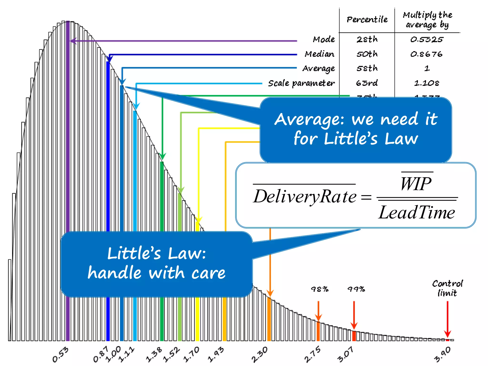
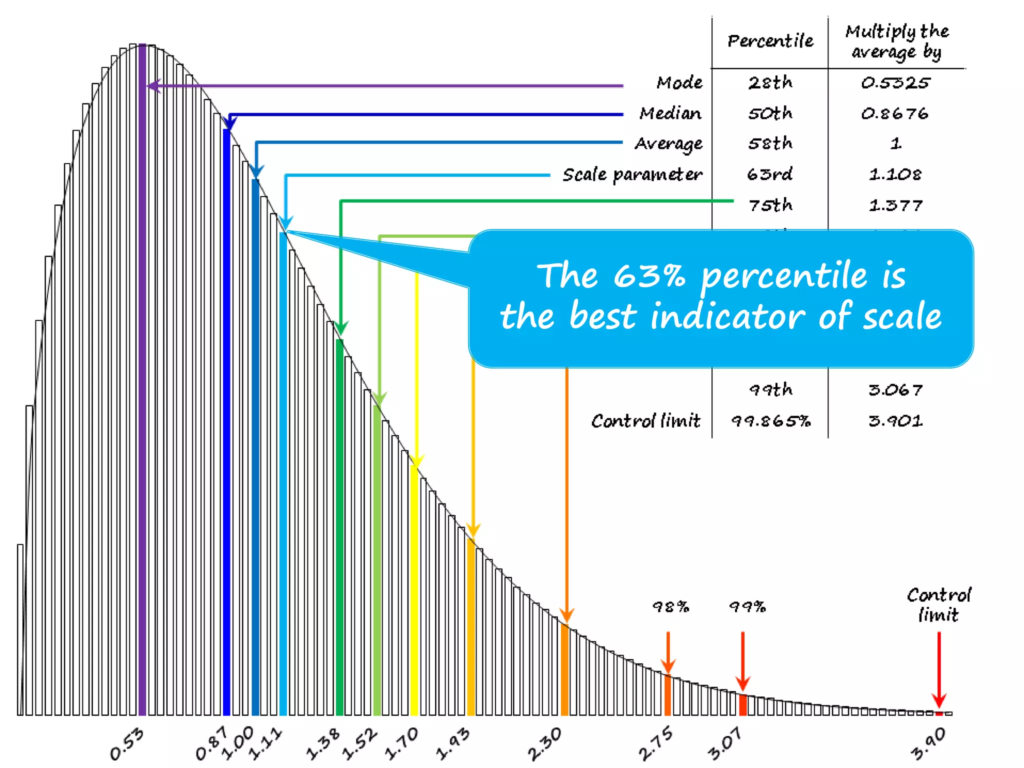
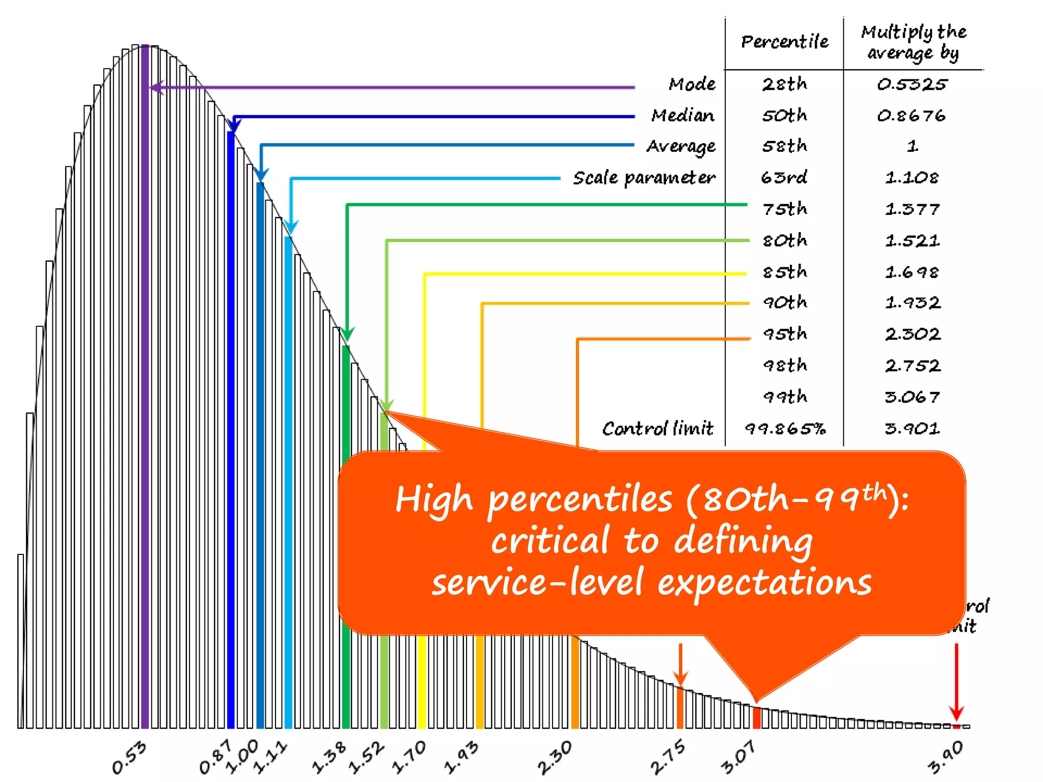
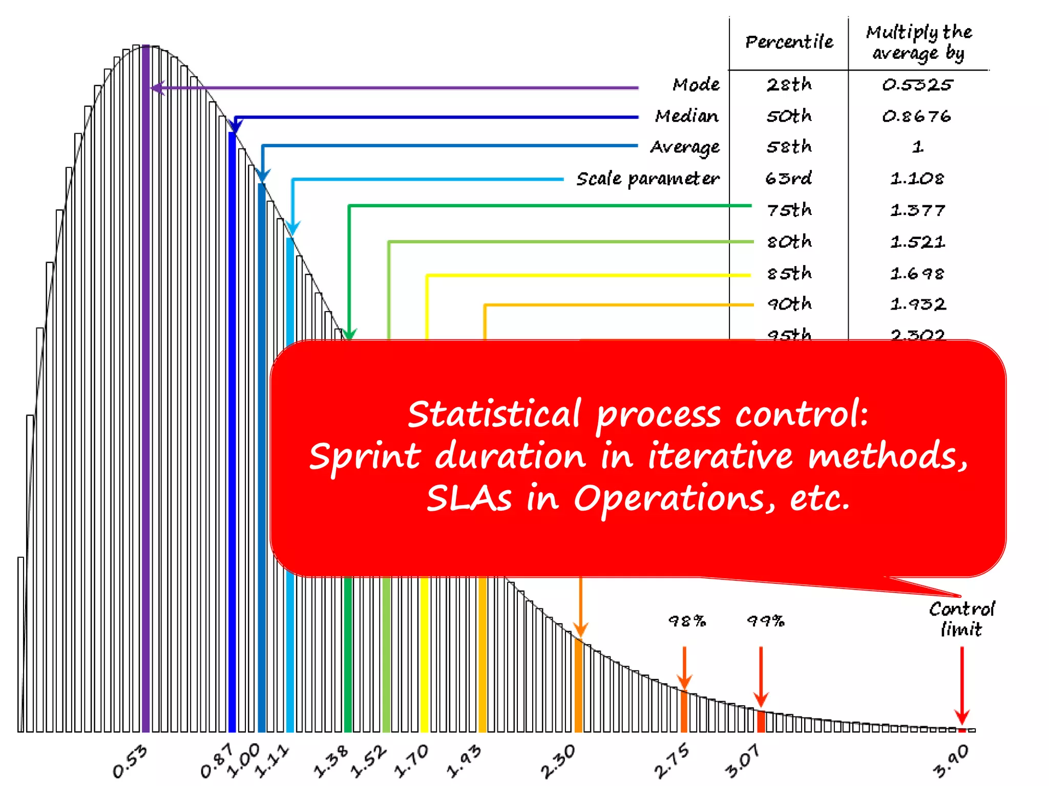
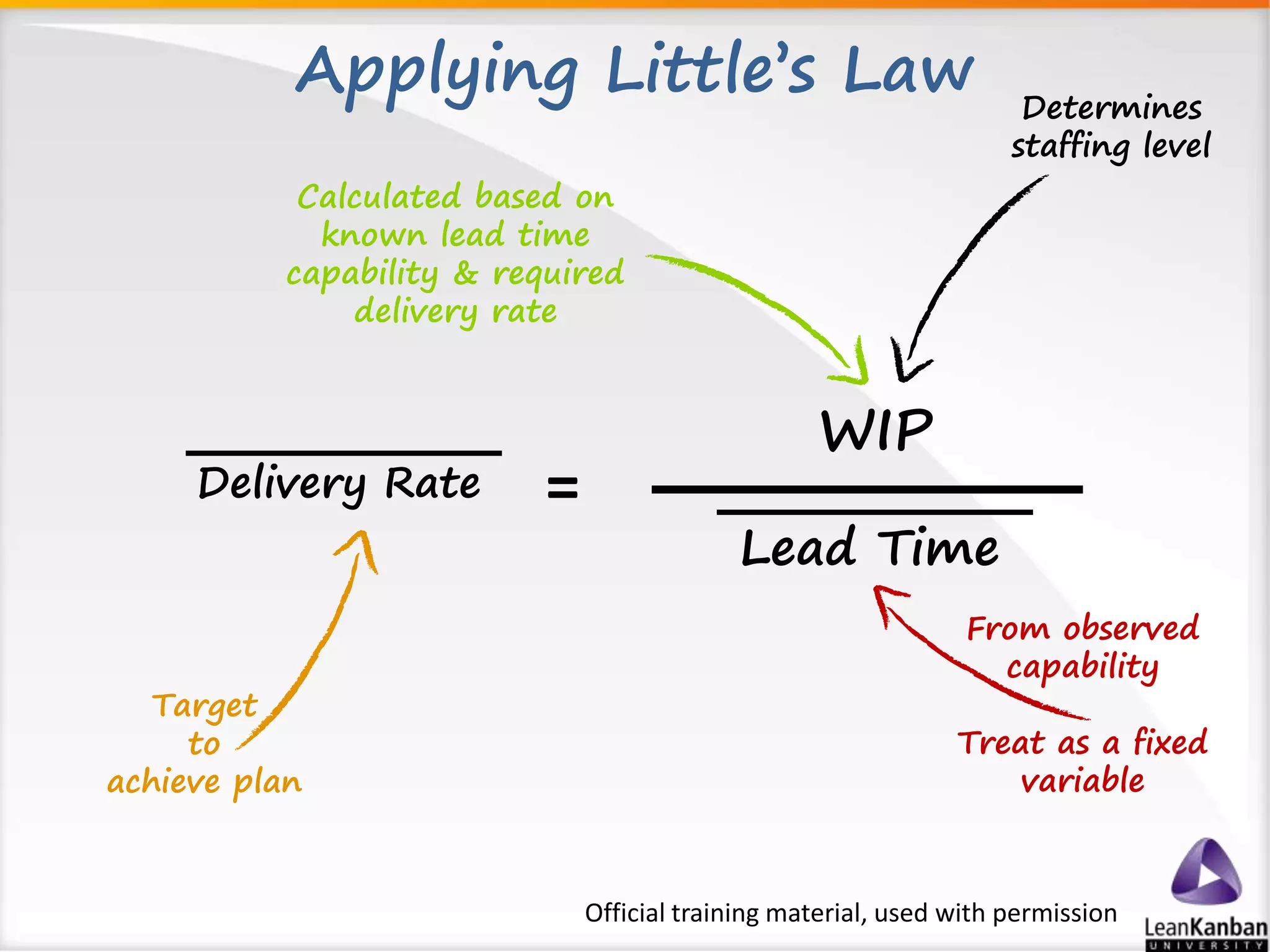
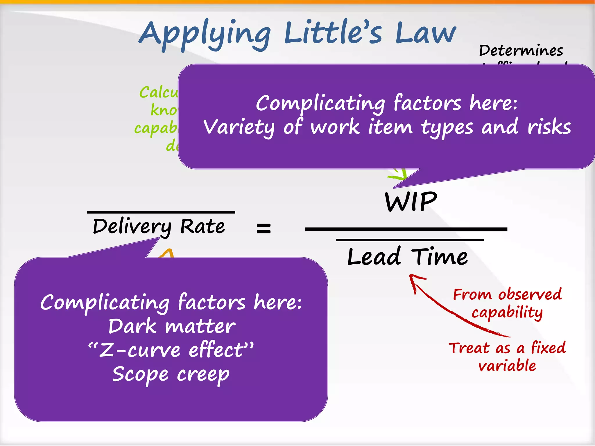
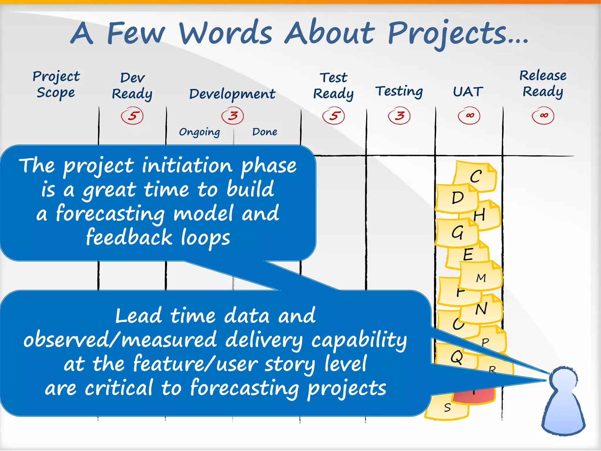
Lead Time: 
What We Know About It 
And How It Can Help Forecast Your Projects 
Alexei Zheglov 
Agile DC 
Washington, October 2014
Alexei Zheglov 
connected-knowledge. 
com 
alex@LeanAtoZ.com
@az1 
#agiledc
Goodhart’s Law 
“When a measure becomes a target, 
it ceases to be a good measure.”
Kanban System Lead Time 
Ideas Input Analysis Delivered 
Queue 
Ready to 
Deliver 
Development Test 
5 2 3 
3 ∞ 
Lead Time 
The First 
Commitment 
Point 
B A 
Discarded 
C 
D
Ask Not 
Ideas Input Analysis Delivered 
Queue 
Ready to 
Deliver 
Development Test 
5 2 3 
3 ∞ 
B A 
Lead Time 
Discarded 
C 
D 
Not “how long will it take?”
Do Ask 
Ideas Input Analysis Delivered 
Queue 
Ready to 
Deliver 
Development Test 
5 2 3 
3 ∞ 
B A 
Lead Time 
Discarded 
C 
D 
When should we start? 
When do we need it?
Decide 
Ideas Input Analysis Delivered 
Queue 
Ready to 
Deliver 
Development Test 
5 2 3 
3 ∞ 
B A 
Lead Time 
Discarded 
C 
D 
One event 
precedes (leads) another one 
by this much
Why? 
Ideas Input Analysis Delivered 
Queue 
Ready to 
Deliver 
Development Test 
5 2 3 
3 ∞ 
Lead Time 
The First 
Commitment 
Point 
B A 
Discarded 
C 
D 
Includes the time the 
work item spent as 
an option 
Depends on the 
transaction costs 
(external to the 
system) 
Measures the 
true delivery 
capability
Customer Lead Time 
Ideas Input Activity 1 Delivered 
Queue 
Output 
Buffer 
Activity 2 Activity 3 
? ? ? 
? ∞ 
Kanban system(s) lead time 
B A 
Customer Lead Time 
+ 
time spent in the unlimited 
buffer(s) 
Discarded 
C 
D
(Local) Cycle Time 
Ideas Input Activity 1 Delivered 
Queue 
Output 
Buffer 
Activity 2 Activity 3 
? ? ? 
? ∞ 
B A 
Discarded 
C 
D 
Cycle time is always local 
Always qualify where 
it is from and to 
Often depends mainly on 
the size of the local effort
Discussion 1: Gaming Metrics 
• Given the goal to reduce the lead time (as we 
have just defined it), what would you do? 
• What would happen, good and bad? 
• How can you game the local cycle time metric? 
• Bonus question: if your delivery time metric 
included the time before commitment, what 
would you be motivated to do?
Flow Efficiency 
Ready 
to Test 
F 
Development Testing 
3 5 3 
E 
J 
G 
D 
GY 
BG 
P1 
DE NP 
AB 
Wait Work Wait Work 
Customer Lead Time 
Ideas 
Ready 
to Dev 
5 
IP 
Done 
UAT 
Ready to 
Deliver 
∞ ∞ 
Work Work Wait 
Official training material, used with permission
Flow Efficiency 
Ready 
to Test 
F 
Development Testing 
3 5 3 
E 
J 
G 
D 
GY 
BG 
P1 
DE NP 
AB 
Wait Work Wait Work 
Customer Lead Time 
Ideas 
Ready 
to Dev 
5 
IP 
Done 
UAT 
Ready to 
Deliver 
∞ ∞ 
Work Work Wait 
Official training material, used with permission 
Work is waiting 
Work is still waiting! 
Multitasking creates 
hidden queues!
Flow Efficiency 
Ready 
to Test 
F 
Development Testing 
3 5 3 
touch time 
E 
J 
G 
D 
flow efficiency   
GY 
BG 
P1 
elapsed time 
DE NP 
AB 
Wait Work Wait Work 
100% 
Customer Lead Time 
Ideas 
Ready 
to Dev 
5 
IP 
Done 
UAT 
Ready to 
Deliver 
∞ ∞ 
Work Work Wait 
Official training material, used with permission
Measuring Flow Efficiency 
Ready 
to Test 
F 
Development Testing 
3 5 3 
E 
J 
G 
D 
GY 
BG 
P1 
DE NP 
AB 
Wait Work Wait Work 
Customer Lead Time 
Ideas 
Ready 
to Dev 
5 
IP 
Done 
UAT 
Ready to 
Deliver 
∞ ∞ 
Sampling 
Work Work Wait 
Official training material, used with permission 
Timesheets are 
not necessary! 
Rough approximations (±5%) 
are often sufficient 
In Aggregate
Measuring Flow Efficiency 
Ready 
to Test 
F 
Development Testing 
3 5 3 
The results are often 
between 1% and 5%* 
The result is not limited to the number! 
E 
J 
G 
D 
What did you decide to do? 
GY 
BG 
P1 
DE NP 
AB 
Wait Work Wait Work 
Customer Lead Time 
Ideas 
Ready 
to Dev 
5 
IP 
Done 
UAT 
Ready to 
Deliver 
∞ ∞ 
Work Work Wait 
*-Zsolt Fabok, Lean Agile Scotland 2012, LKFR12; Hakan Forss, LKFR13
If the Flow Efficiency Is 5%... 
If... Before After Improvement 
Hire 10x engineers 100 95.5 +4.7% 
The task is three 
times bigger 100 110 -9.1% 
The task is three 
times smaller 100 96.7 +3.4% 
Reduce delays by 
half 100 52.5 +90%
Consequences of Low Flow Efficiency 
• Lead time is hard to fudge 
• Lead time improves primarily due to 
system-level improvements 
• The lead time data from your previous 
projects likely relevant to the upcoming 
one
Goodhart’s Law’s 
Corollary 
Measuring the delivery time 
cannot be separated from 
understanding commitment.
Start Measuring?
Discussion 2: Measuring Lead Time 
• Do you already collect lead time data? 
• If not, do you already have these data available 
somewhere, waiting for you to discover them? 
• If not, would it be difficult or easy to start? 
• What would you do differently in your company 
with respect to lead time data after this 
presentation?
probabilistic 
Deterministic approach 
to a probabilistic process? 
!!!
20 
18 
16 
14 
12 
10 
8 
6 
4 
2 
0 
Example 
0-4 5-9 10-14 15-19 20-24 25-29 30-34 35-39 40-44 45-49 50-54 55-59 60-64 65-69 70-74 75-79 80-84 85-89 95-99 100-104
20 
18 
16 
14 
12 
10 
8 
6 
4 
2 
0 
Example 
Best-fit distribution: 
Weibull with 
shape parameter k=1.62 
0-4 5-9 10-14 15-19 20-24 25-29 30-34 35-39 40-44 45-49 50-54 55-59 60-64 65-69 70-74 75-79 80-84 85-89 95-99 100-104
Heterogeneous Demand 
Ideas Input Analysis Delivered 
Queue 
Ready to 
Deliver 
Development Test 
5 2 3 
3 ∞ 
B A 
Discarded 
C 
D 
E 
G 
F 
H 
Demand placed upon our system 
is differentiated 
by type of work and risk
Drill down by project type 
0 
5 
10 
15 
20 
0-4 
5-9 
10-14 
15-19 
20-24 
25-29 
30-34 
35-39 
40-44 
45-49 
50-54 
55-59 
60-64 
65-69 
70-74 
75-79 
80-84 
85-89 
95-99 
100-104 
0 
2 
4 
6 
8 
10 
12 
14 
16 
18 
20 
Mixed data from 
different types of 
projects
4 types, 4 different distributions 
0 
5 
10 
15 
20 
0-4 
5-9 
10-14 
15-19 
20-24 
25-29 
30-34 
35-39 
40-44 
45-49 
50-54 
55-59 
60-64 
65-69 
70-74 
75-79 
80-84 
85-89 
95-99 
100-104 
0 
5 
10 
15 
20 
0-4 
5-9 
10-14 
15-19 
20-24 
25-29 
30-34 
35-39 
40-44 
45-49 
50-54 
55-59 
60-64 
65-69 
70-74 
75-79 
80-84 
85-89 
95-99 
100-104 
0 
2 
4 
6 
8 
10 
12 
14 
16 
18 
5-9 
10-14 
15-19 
20-24 
25-29 
30-34 
35-39 
40-44 
45-49 
50-54 
55-59 
60-64 
65-69 
75-79 
80-84 
85-89 
100-104 
0 
1 
2 
3 
4 
5 
6 
0-4 
5-9 
10-14 
15-19 
20-24 
25-29 
40-44 
55-59 
60-64 
65-69 
70-74 
75-79 
95-99 
... 
...
Delivery Expectations 
0 
5 
10 
15 
20 
0-4 
5-9 
10-14 
15-19 
20-24 
25-29 
30-34 
35-39 
40-44 
45-49 
50-54 
55-59 
60-64 
65-69 
70-74 
75-79 
80-84 
85-89 
95-99 
100-104 
0 
5 
10 
15 
20 
0-4 
5-9 
10-14 
15-19 
20-24 
25-29 
30-34 
35-39 
40-44 
45-49 
50-54 
55-59 
60-64 
65-69 
70-74 
75-79 
80-84 
85-89 
95-99 
100-104 
Shape Average In 98% 
1.62 
1.23 
1.65 
3.22 
In 85% of cases 
30 d 
35 d 
40 d 
56 d 
<51 
<63 
<68 
<78 
<83 
<112* 
<110* 
<99
Delivery Expectations 
0 
5 
10 
15 
20 
0-4 
5-9 
10-14 
15-19 
20-24 
25-29 
30-34 
35-39 
40-44 
45-49 
50-54 
55-59 
60-64 
65-69 
70-74 
75-79 
80-84 
85-89 
95-99 
100-104 
0 
5 
10 
15 
20 
0-4 
5-9 
10-14 
15-19 
20-24 
25-29 
30-34 
35-39 
40-44 
45-49 
50-54 
55-59 
60-64 
65-69 
70-74 
75-79 
80-84 
85-89 
95-99 
100-104 
Shape Average In 98% 
1.62 
1.23 
1.65 
3.22 
In 85% of cases 
30 d 
35 d 
40 d 
56 d 
<51 
<63 
<68 
<78 
<83 
<112* 
<110* 
<99 
The averages are insufficient 
to specify delivery capabilities! 
The average says nothing 
about variability! Needed: 
the average and a high 
percentile (usually 80-99%)
Another Example 
12 
10 
8 
6 
4 
2 
0 
Development 
0-2.5 2.5-5 5-7.5 7.5-10 10-12.5 12.5-15 15-17.5 25-27.5 
14 
12 
10 
8 
6 
4 
2 
0 
Support 
0-3 3-6 6-9 9-12 12-15 15-18 
Shape: 1.16 Shape: 0.71
Weibull Distributions 
Occur Frequently 
New product development Operations, support (k<1) 
(k>1)
Weibull Distributions 
Occur Frequently 
New product development Operations, support (k<1) 
(k>1) 
The unique signature 
of your process
How to “Read” a Distribution 
Bias 
Feedback 
Forecast 
Scale 
Expectations 
Control
Mode: how we remember 
the “typical” delivered work item. 
Trouble: it’s a very low percentile. 
18-28% common.
Median: 50% more, 50% less. 
Perfect for creating 
very short feedback loops
Average: we need it 
for Little’s Law 
WIP 
LeadTime 
DeliveryRate  
Little’s Law: 
handle with care
The 63% percentile is 
the best indicator of scale
High percentiles (80th-99th): 
critical to defining 
service-level expectations
Statistical process control: 
Sprint duration in iterative methods, 
SLAs in Operations, etc.
Forecasting Cards
While I Was Preparing This Presentation, 
Somebody Sent Me This...
Discussion 3: 
Probabilistic or Deterministic? 
• Would you describe the prevailing approach in 
your organization as probabilistic or 
deterministic? 
• Is the expected answer to “how long will it take?” 
a single number? 
• Can you instead ask, “when do we need it?” and 
“when should we start?” 
• Can you make decisions given distributions of 
probabilities?
A Few Words About Projects… 
Test 
Ready 
D 
S 
R 
E 
Q 
P 
O 
N 
F 
I 
G 
M 
Dev 
Ready 
5 
Development Testing 
Ongoing 
3 5 3 
Done 
UAT 
Release 
Ready 
∞ ∞ 
Project 
Scope 
Official training material, used with permission
Applying Little’s Law 
Calculated based on 
known lead time 
capability & required 
Delivery Rate 
WIP 
Lead Time 
= 
From observed 
capability 
Treat as a fixed 
variable 
Target 
to 
achieve plan 
delivery rate 
Determines 
staffing level 
Official training material, used with permission
Applying Little’s Law 
Calculated based on 
known lead time 
capability & required 
Delivery Rate 
WIP 
Lead Time 
= 
From observed 
capability 
Treat as a fixed 
variable 
Target 
to 
achieve plan 
delivery rate 
Determines 
staffing level 
Complicating factors here: 
Dark matter 
“Z-curve effect” 
Scope creep 
Complicating factors here: 
Variety of work item types and risks
A Few Words About Projects… 
Test 
Ready 
D 
S 
R 
E 
Q 
P 
O 
N 
F 
I 
G 
M 
Dev 
Ready 
5 
Development Testing 
Ongoing 
3 5 3 
Done 
UAT 
Release 
Ready 
∞ ∞ 
Project 
Scope 
The project initiation phase 
is a great time to build 
a forecasting model and 
feedback loops 
Lead time data and 
observed/measured delivery capability 
at the feature/user story level 
are critical to forecasting projects
New Kanban Book 
Mike Burrows
Influencers 
Troy Magennis Dimitar Bakardzhiev David J Anderson 
Dan Vacanti Dave White Frank Vega
Discussion 4: What Now? 
• What new ideas have your learned in this 
session today? 
• What will you do differently when you return to 
your office tomorrow?
Alexei Zheglov 
connected-knowledge.com (blog) 
alex@LeanAtoZ.com 
@az1

Agile DC Lead Time

  • 1.
    Lead Time: WhatWe Know About It And How It Can Help Forecast Your Projects Alexei Zheglov Agile DC Washington, October 2014
  • 2.
  • 3.
  • 4.
    Goodhart’s Law “Whena measure becomes a target, it ceases to be a good measure.”
  • 5.
    Kanban System LeadTime Ideas Input Analysis Delivered Queue Ready to Deliver Development Test 5 2 3 3 ∞ Lead Time The First Commitment Point B A Discarded C D
  • 6.
    Ask Not IdeasInput Analysis Delivered Queue Ready to Deliver Development Test 5 2 3 3 ∞ B A Lead Time Discarded C D Not “how long will it take?”
  • 7.
    Do Ask IdeasInput Analysis Delivered Queue Ready to Deliver Development Test 5 2 3 3 ∞ B A Lead Time Discarded C D When should we start? When do we need it?
  • 8.
    Decide Ideas InputAnalysis Delivered Queue Ready to Deliver Development Test 5 2 3 3 ∞ B A Lead Time Discarded C D One event precedes (leads) another one by this much
  • 9.
    Why? Ideas InputAnalysis Delivered Queue Ready to Deliver Development Test 5 2 3 3 ∞ Lead Time The First Commitment Point B A Discarded C D Includes the time the work item spent as an option Depends on the transaction costs (external to the system) Measures the true delivery capability
  • 10.
    Customer Lead Time Ideas Input Activity 1 Delivered Queue Output Buffer Activity 2 Activity 3 ? ? ? ? ∞ Kanban system(s) lead time B A Customer Lead Time + time spent in the unlimited buffer(s) Discarded C D
  • 11.
    (Local) Cycle Time Ideas Input Activity 1 Delivered Queue Output Buffer Activity 2 Activity 3 ? ? ? ? ∞ B A Discarded C D Cycle time is always local Always qualify where it is from and to Often depends mainly on the size of the local effort
  • 12.
    Discussion 1: GamingMetrics • Given the goal to reduce the lead time (as we have just defined it), what would you do? • What would happen, good and bad? • How can you game the local cycle time metric? • Bonus question: if your delivery time metric included the time before commitment, what would you be motivated to do?
  • 13.
    Flow Efficiency Ready to Test F Development Testing 3 5 3 E J G D GY BG P1 DE NP AB Wait Work Wait Work Customer Lead Time Ideas Ready to Dev 5 IP Done UAT Ready to Deliver ∞ ∞ Work Work Wait Official training material, used with permission
  • 14.
    Flow Efficiency Ready to Test F Development Testing 3 5 3 E J G D GY BG P1 DE NP AB Wait Work Wait Work Customer Lead Time Ideas Ready to Dev 5 IP Done UAT Ready to Deliver ∞ ∞ Work Work Wait Official training material, used with permission Work is waiting Work is still waiting! Multitasking creates hidden queues!
  • 15.
    Flow Efficiency Ready to Test F Development Testing 3 5 3 touch time E J G D flow efficiency   GY BG P1 elapsed time DE NP AB Wait Work Wait Work 100% Customer Lead Time Ideas Ready to Dev 5 IP Done UAT Ready to Deliver ∞ ∞ Work Work Wait Official training material, used with permission
  • 16.
    Measuring Flow Efficiency Ready to Test F Development Testing 3 5 3 E J G D GY BG P1 DE NP AB Wait Work Wait Work Customer Lead Time Ideas Ready to Dev 5 IP Done UAT Ready to Deliver ∞ ∞ Sampling Work Work Wait Official training material, used with permission Timesheets are not necessary! Rough approximations (±5%) are often sufficient In Aggregate
  • 17.
    Measuring Flow Efficiency Ready to Test F Development Testing 3 5 3 The results are often between 1% and 5%* The result is not limited to the number! E J G D What did you decide to do? GY BG P1 DE NP AB Wait Work Wait Work Customer Lead Time Ideas Ready to Dev 5 IP Done UAT Ready to Deliver ∞ ∞ Work Work Wait *-Zsolt Fabok, Lean Agile Scotland 2012, LKFR12; Hakan Forss, LKFR13
  • 18.
    If the FlowEfficiency Is 5%... If... Before After Improvement Hire 10x engineers 100 95.5 +4.7% The task is three times bigger 100 110 -9.1% The task is three times smaller 100 96.7 +3.4% Reduce delays by half 100 52.5 +90%
  • 19.
    Consequences of LowFlow Efficiency • Lead time is hard to fudge • Lead time improves primarily due to system-level improvements • The lead time data from your previous projects likely relevant to the upcoming one
  • 20.
    Goodhart’s Law’s Corollary Measuring the delivery time cannot be separated from understanding commitment.
  • 21.
  • 22.
    Discussion 2: MeasuringLead Time • Do you already collect lead time data? • If not, do you already have these data available somewhere, waiting for you to discover them? • If not, would it be difficult or easy to start? • What would you do differently in your company with respect to lead time data after this presentation?
  • 23.
    probabilistic Deterministic approach to a probabilistic process? !!!
  • 24.
    20 18 16 14 12 10 8 6 4 2 0 Example 0-4 5-9 10-14 15-19 20-24 25-29 30-34 35-39 40-44 45-49 50-54 55-59 60-64 65-69 70-74 75-79 80-84 85-89 95-99 100-104
  • 25.
    20 18 16 14 12 10 8 6 4 2 0 Example Best-fit distribution: Weibull with shape parameter k=1.62 0-4 5-9 10-14 15-19 20-24 25-29 30-34 35-39 40-44 45-49 50-54 55-59 60-64 65-69 70-74 75-79 80-84 85-89 95-99 100-104
  • 26.
    Heterogeneous Demand IdeasInput Analysis Delivered Queue Ready to Deliver Development Test 5 2 3 3 ∞ B A Discarded C D E G F H Demand placed upon our system is differentiated by type of work and risk
  • 27.
    Drill down byproject type 0 5 10 15 20 0-4 5-9 10-14 15-19 20-24 25-29 30-34 35-39 40-44 45-49 50-54 55-59 60-64 65-69 70-74 75-79 80-84 85-89 95-99 100-104 0 2 4 6 8 10 12 14 16 18 20 Mixed data from different types of projects
  • 28.
    4 types, 4different distributions 0 5 10 15 20 0-4 5-9 10-14 15-19 20-24 25-29 30-34 35-39 40-44 45-49 50-54 55-59 60-64 65-69 70-74 75-79 80-84 85-89 95-99 100-104 0 5 10 15 20 0-4 5-9 10-14 15-19 20-24 25-29 30-34 35-39 40-44 45-49 50-54 55-59 60-64 65-69 70-74 75-79 80-84 85-89 95-99 100-104 0 2 4 6 8 10 12 14 16 18 5-9 10-14 15-19 20-24 25-29 30-34 35-39 40-44 45-49 50-54 55-59 60-64 65-69 75-79 80-84 85-89 100-104 0 1 2 3 4 5 6 0-4 5-9 10-14 15-19 20-24 25-29 40-44 55-59 60-64 65-69 70-74 75-79 95-99 ... ...
  • 29.
    Delivery Expectations 0 5 10 15 20 0-4 5-9 10-14 15-19 20-24 25-29 30-34 35-39 40-44 45-49 50-54 55-59 60-64 65-69 70-74 75-79 80-84 85-89 95-99 100-104 0 5 10 15 20 0-4 5-9 10-14 15-19 20-24 25-29 30-34 35-39 40-44 45-49 50-54 55-59 60-64 65-69 70-74 75-79 80-84 85-89 95-99 100-104 Shape Average In 98% 1.62 1.23 1.65 3.22 In 85% of cases 30 d 35 d 40 d 56 d <51 <63 <68 <78 <83 <112* <110* <99
  • 30.
    Delivery Expectations 0 5 10 15 20 0-4 5-9 10-14 15-19 20-24 25-29 30-34 35-39 40-44 45-49 50-54 55-59 60-64 65-69 70-74 75-79 80-84 85-89 95-99 100-104 0 5 10 15 20 0-4 5-9 10-14 15-19 20-24 25-29 30-34 35-39 40-44 45-49 50-54 55-59 60-64 65-69 70-74 75-79 80-84 85-89 95-99 100-104 Shape Average In 98% 1.62 1.23 1.65 3.22 In 85% of cases 30 d 35 d 40 d 56 d <51 <63 <68 <78 <83 <112* <110* <99 The averages are insufficient to specify delivery capabilities! The average says nothing about variability! Needed: the average and a high percentile (usually 80-99%)
  • 31.
    Another Example 12 10 8 6 4 2 0 Development 0-2.5 2.5-5 5-7.5 7.5-10 10-12.5 12.5-15 15-17.5 25-27.5 14 12 10 8 6 4 2 0 Support 0-3 3-6 6-9 9-12 12-15 15-18 Shape: 1.16 Shape: 0.71
  • 32.
    Weibull Distributions OccurFrequently New product development Operations, support (k<1) (k>1)
  • 33.
    Weibull Distributions OccurFrequently New product development Operations, support (k<1) (k>1) The unique signature of your process
  • 34.
    How to “Read”a Distribution Bias Feedback Forecast Scale Expectations Control
  • 35.
    Mode: how weremember the “typical” delivered work item. Trouble: it’s a very low percentile. 18-28% common.
  • 36.
    Median: 50% more,50% less. Perfect for creating very short feedback loops
  • 37.
    Average: we needit for Little’s Law WIP LeadTime DeliveryRate  Little’s Law: handle with care
  • 38.
    The 63% percentileis the best indicator of scale
  • 39.
    High percentiles (80th-99th): critical to defining service-level expectations
  • 40.
    Statistical process control: Sprint duration in iterative methods, SLAs in Operations, etc.
  • 41.
  • 42.
    While I WasPreparing This Presentation, Somebody Sent Me This...
  • 43.
    Discussion 3: Probabilisticor Deterministic? • Would you describe the prevailing approach in your organization as probabilistic or deterministic? • Is the expected answer to “how long will it take?” a single number? • Can you instead ask, “when do we need it?” and “when should we start?” • Can you make decisions given distributions of probabilities?
  • 44.
    A Few WordsAbout Projects… Test Ready D S R E Q P O N F I G M Dev Ready 5 Development Testing Ongoing 3 5 3 Done UAT Release Ready ∞ ∞ Project Scope Official training material, used with permission
  • 45.
    Applying Little’s Law Calculated based on known lead time capability & required Delivery Rate WIP Lead Time = From observed capability Treat as a fixed variable Target to achieve plan delivery rate Determines staffing level Official training material, used with permission
  • 46.
    Applying Little’s Law Calculated based on known lead time capability & required Delivery Rate WIP Lead Time = From observed capability Treat as a fixed variable Target to achieve plan delivery rate Determines staffing level Complicating factors here: Dark matter “Z-curve effect” Scope creep Complicating factors here: Variety of work item types and risks
  • 47.
    Applying Little’s Law Calculated based on known lead time capability & required Delivery Rate WIP Lead Time = From observed capability Treat as a fixed variable Target to achieve plan delivery rate Determines staffing level Complicating factors here: Dark matter “Z-curve effect” Scope creep Complicating factors here: Variety of work item types and risks
  • 48.
    A Few WordsAbout Projects… Test Ready D S R E Q P O N F I G M Dev Ready 5 Development Testing Ongoing 3 5 3 Done UAT Release Ready ∞ ∞ Project Scope The project initiation phase is a great time to build a forecasting model and feedback loops Lead time data and observed/measured delivery capability at the feature/user story level are critical to forecasting projects
  • 49.
    New Kanban Book Mike Burrows
  • 50.
    Influencers Troy MagennisDimitar Bakardzhiev David J Anderson Dan Vacanti Dave White Frank Vega
  • 51.
    Discussion 4: WhatNow? • What new ideas have your learned in this session today? • What will you do differently when you return to your office tomorrow?
  • 52.
    Alexei Zheglov connected-knowledge.com(blog) alex@LeanAtoZ.com @az1