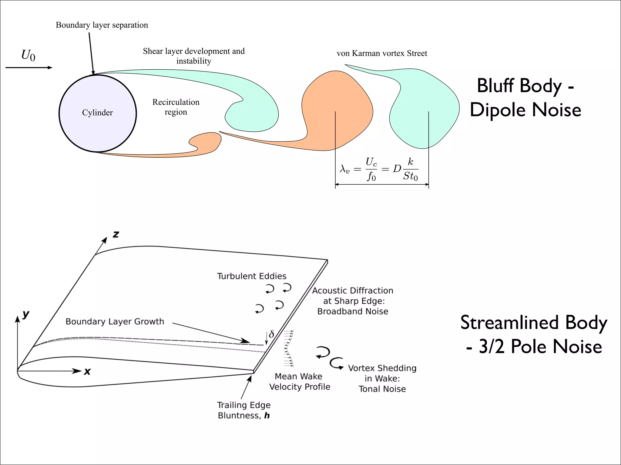
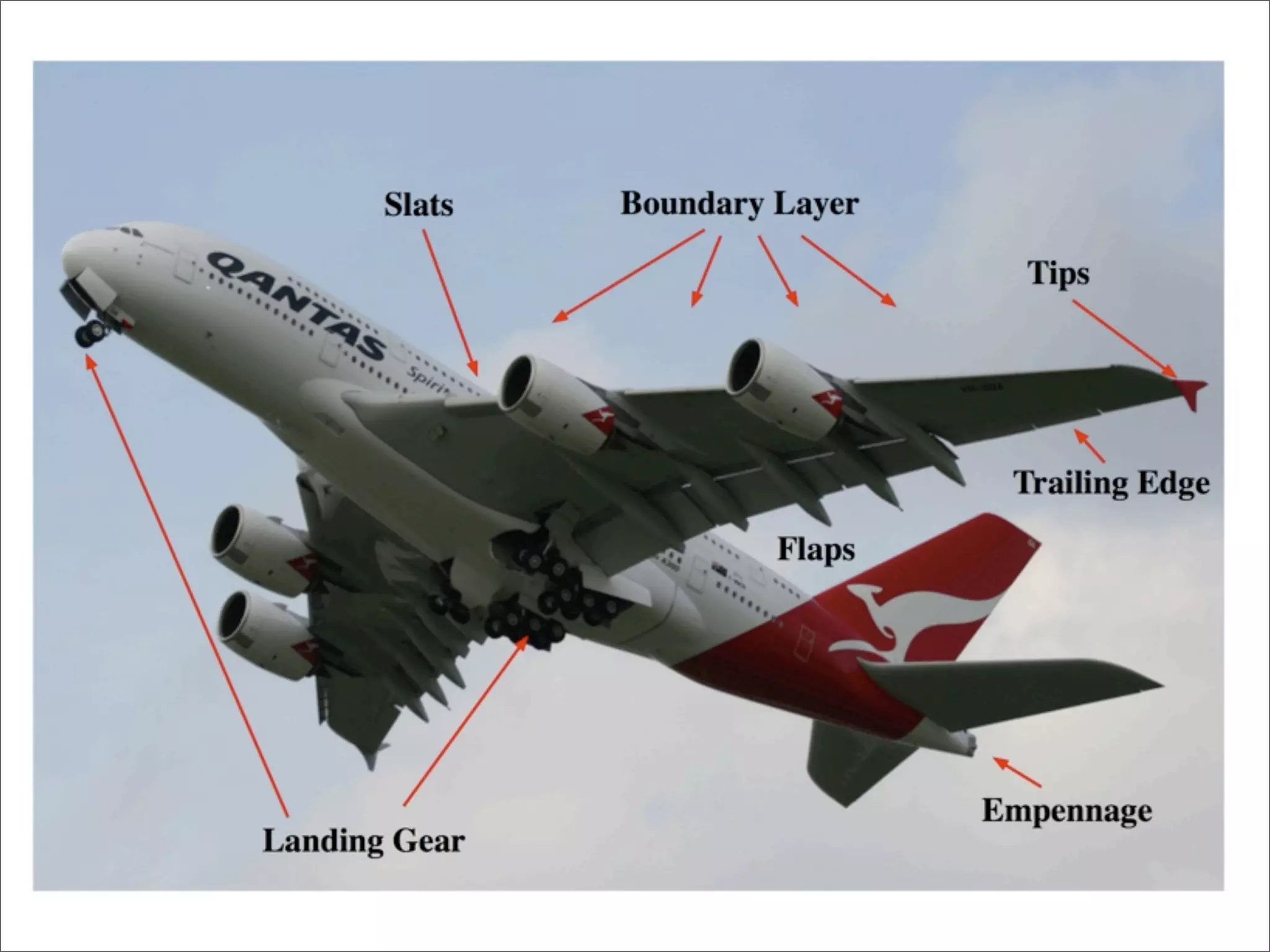
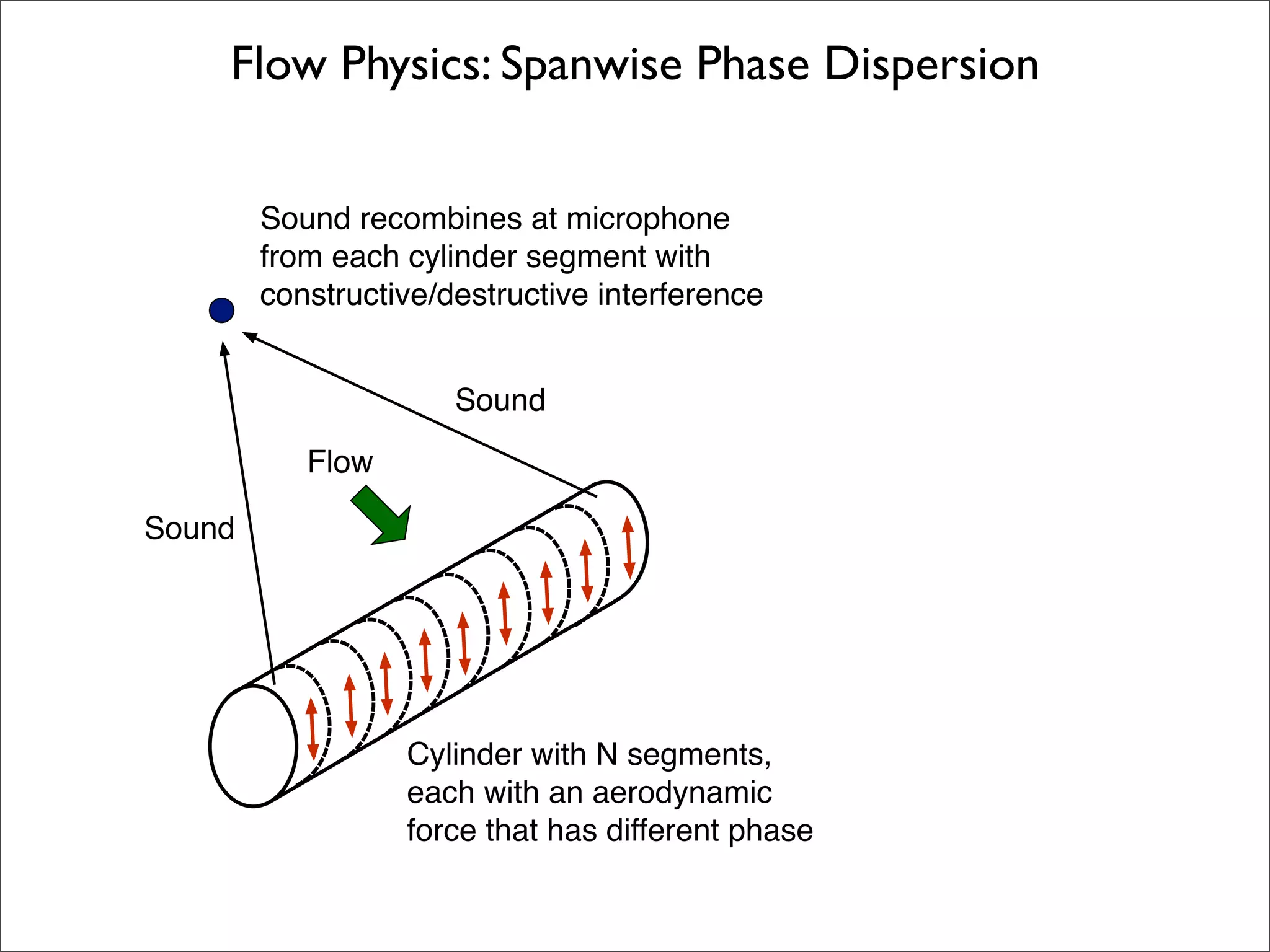
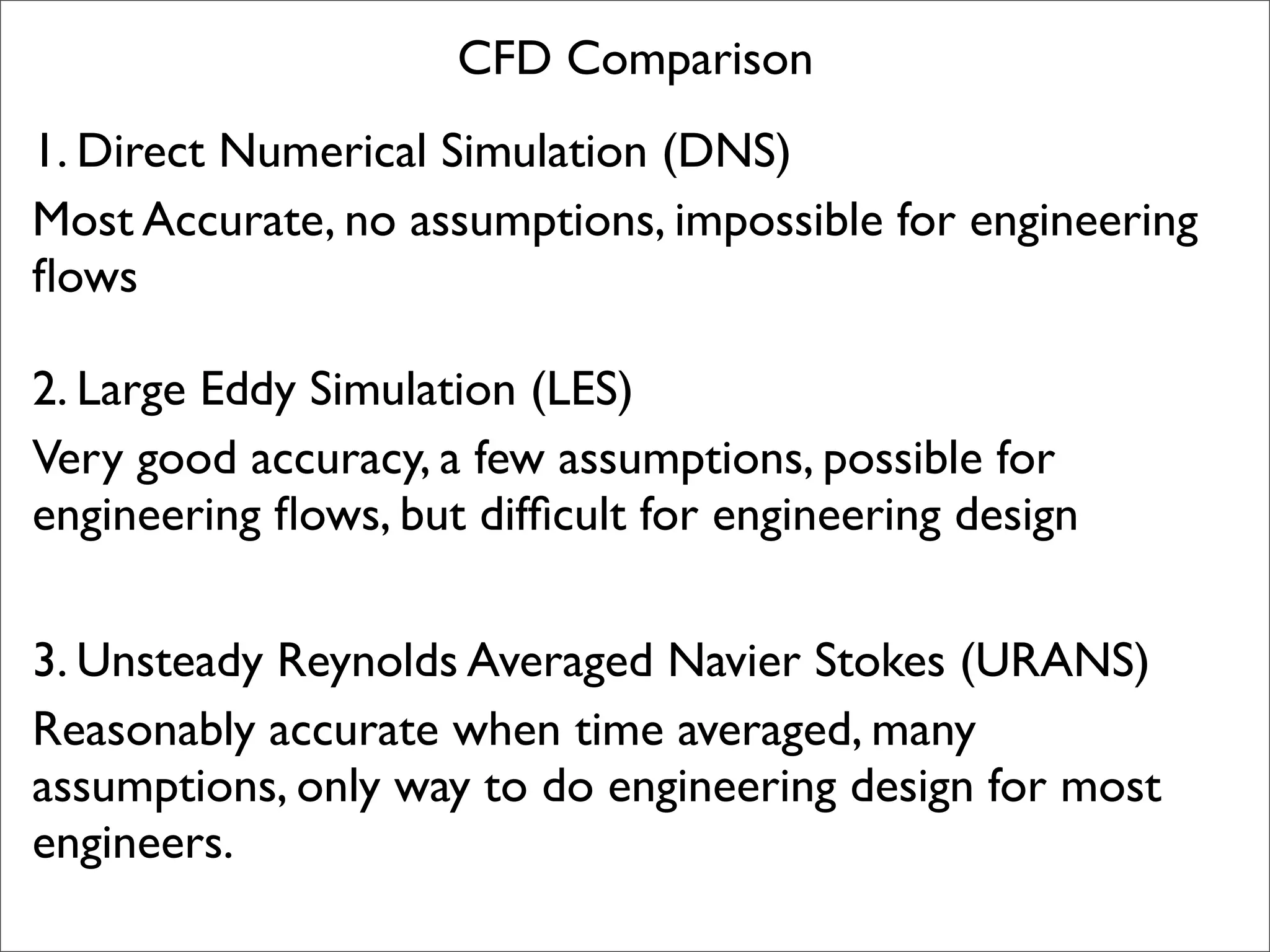
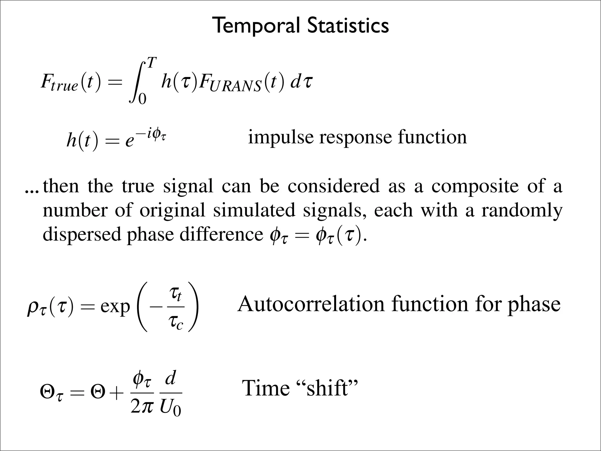
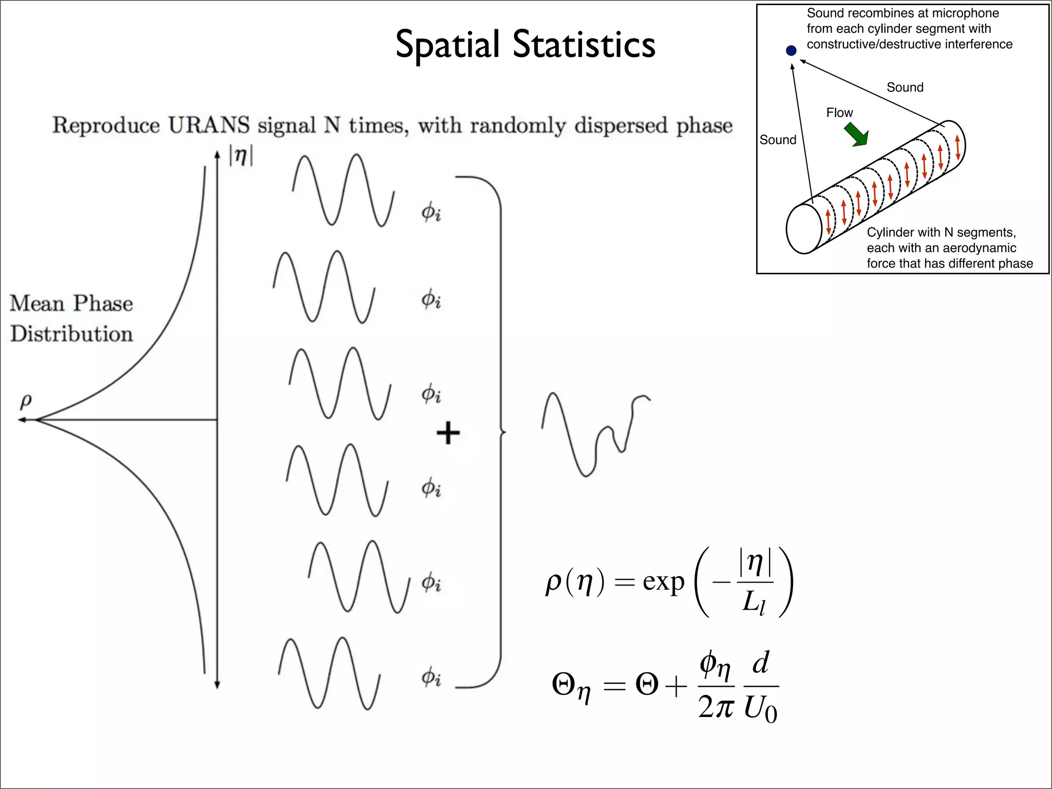
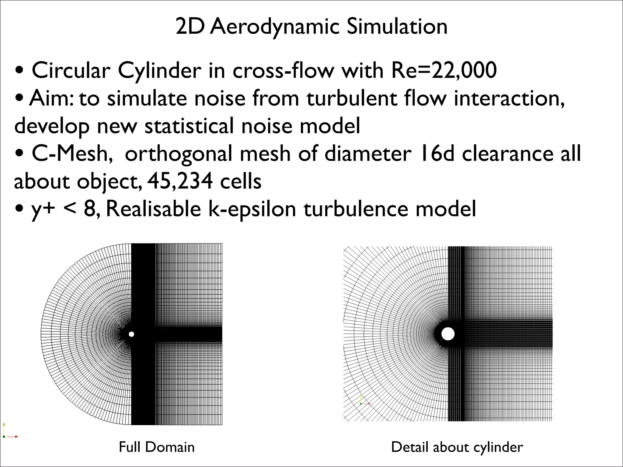
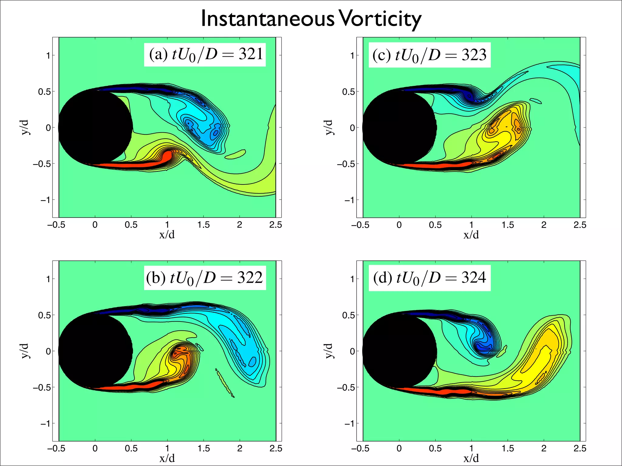
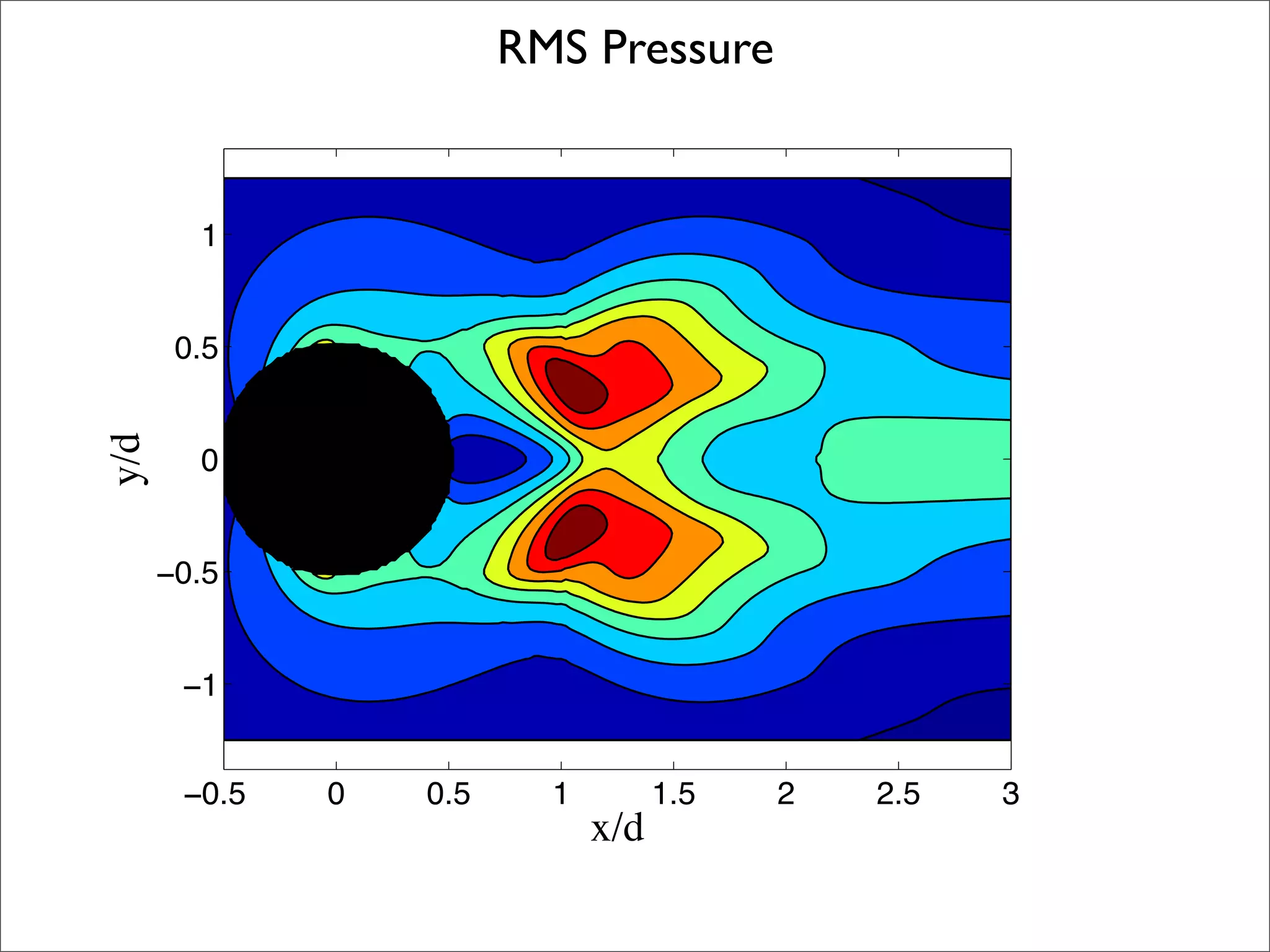
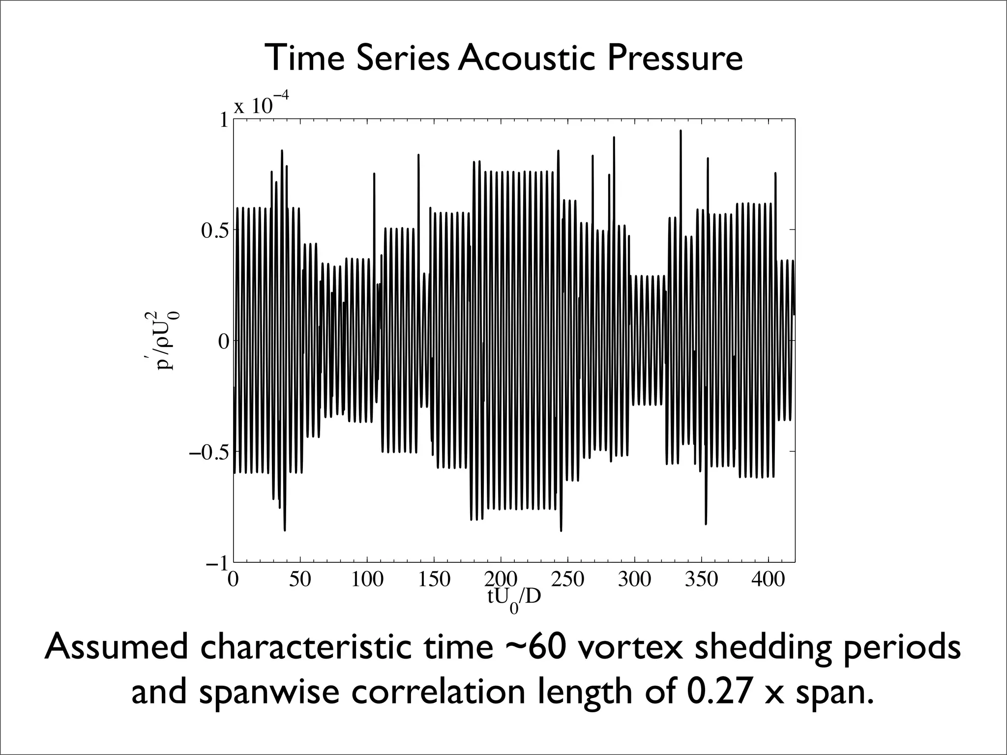
The document summarizes a presentation on aeroacoustic simulation of bluff body noise using a hybrid statistical method. It discusses limitations of conventional computational fluid dynamics methods for noise prediction and introduces a new statistical correction method to improve noise simulation results from unsteady Reynolds-averaged Navier Stokes simulations. Key results from applying the statistical correction to simulations of circular cylinder noise are also summarized.

1. School of Mechanical Engineering
Tuesday, November 10, 2009
Aeroacoustic simulation of bluff
body noise using a hybrid statistical
method
Con Doolan
School of Mechanical Engineering
University of Adelaide, SA, 5005
ACOUSTICS 2009
Life Impact The University of Adelaide

2. Summary
• Bluff Body Noise - What is it?
• Why is it important?
• Physics controlling flow and noise
• Simulation methods - limitations for
engineers
• Statistical Correction
• Results

3. 
 
U0 
Bluff Body -

  Dipole Noise
Uc k
λv = =D
f0 St0
Streamlined Body
- 3/2 Pole Noise

5. LES/Flow Simulation Upper Drag Link
COMPUTATIONAL AEROACOUSTIC ANALYSIS OF A
1/4 SCALE G550 NOSE LANDING GEAR AND
COMPARISON TO NASA & UFL WIND TUNNEL DATA
Thomas Van de Ven* and John Louis**
Gulfstream Aerospace Corporation
Savannah, GA
Dean Palfreyman*** and Fred Mendonça****
CD-adapco
AIAA Paper 2009-3359 (Miami, 2009)
Lower Drag Link

6. Automotive Bluff Body Noise
Large Eddy Simulation
Sandeep Sovani, FLUENT, 2005
Beamforming
Christensen et al. Beamforming. Bruel & Kjaer
Technical Review (2004) vol. No. 1 – 2004

7. Subs and Trains

8. an be simplified to predict the acoustic far field (represented
Theory
s a density fluctuation ρ ) generated at an observation point by 2
Compact Aeroacoustic equation (Curle 1955) 4πc
form of Curle’s Noise: Curle’s Theory
ustically compact force F applied on a compressible fluid that 0 ρ
fluctuating point ˜
predict the23–25 November 2009, Adelaide, Austral
implifiedIfto body is compact, then the noise (density
initially atarest acoustic far field (represented
fluctuation ρ )is function of the force acting on it 2009, t
sity23–25 Novembera2009, Adelaide, Australia point by (Fi)are theA
) generated at an observation November
23–25 where
en the propagation time between points onfluidapplied on is zer
˜ applied on compressible the surface the flu
ting point force F Brief Article
∂ 0.
a that
in the above points the propagation time ∂ an estimate of th
ly at rest4πc2 ρ equation d →surface 1 xi between points on th
then on the Fi Therefore, Fi (air) at rest. The
time between (x,t) = −
0 ˜ = is zero, (4)
2 be∂t 0. to the compact b
ror due→ 0. Therefore,∂an estimate0of the made by dividin
to a compactthe above equation d → The distance bet
or in assumption c r
tion d Region about cylinder xi r can Therefore, an
(b)
q. 2 by itself but error be =0. a compact assumption can (takin
with due to Author
The Inby dividing
d made dB,this expression is by the
act assumption can aerodynamic1simulation described be m
Thecomponent) ∂ F with the (taking
2 error (dB) associated
4πc0 0. In
ith d this r =
i ∂ the
e real=arex,t)dB,Eq. 2 expression xis compact assumption is:
omputational the threefor by iitself but with Fi = resulting forceexpre
here Fiρ ( ˜ grid= − vector components ofd 0. Intaken at the retard
used dB, this
(4)
andreal component) ∂t
∂ i 2 sound of the medium
pplied on the fluid the xc0 is the speed of 2009
November 010, c r
E = 434,783 10 cos(πStM) with URANS simula
h times. This corresponds to 20 log time steps and
˜ A
respect (3
air) at rest. The observation point is x measured (F (t), used to ca
E = 20of the cos(πStM)
log10 cylinder).
i
o0are the three vector(in this case, thethe resulting force acoustic
the compact body with 439 non-dimensional
vortex shedding cycles components of centre
=shedding 10 cos(πStM) the maximum frequency is limite
20 log period. (3) compact
per thecase considered here, of soundobservation point is is we
onthe fluid and c0For the speedconsideredof the medium
r
he distance between the case and the here, the maximum freq
is the body However, it
a Strouhal number,pointThis number, Stwith respect number o
The x work:brackets f Mach 2 simulati
escribed by the distance r.= is d/U0 is limitedad/U a value a M
St frequency = 2 and denote = of and
f square
ed here, observation Strouhal˜ measured =
est.SIMULATION to a
The the maximum types
TIC METHOD 0
06. Thisf results thisand aMtE centre an error E 1 the vortex s
0.06. Θ the r/cin
ompactthed/U(in intimeThisMach number of
mate the assum
r, St at body 0 = 2an error − 1 .dB. the cylinder). poor noise
ken
= retarded case,=results 0 of Therefore in Theref
= 0.06 ing dB.
on of compactness isof compactness is the presentis the pre
Acoustic Assumption appropriate for
appropriate work. No
an error E 1 dB. Therefore the assump- point for results fr
ance between the body and the observation
tion ciencies

9. Flow Physics: Surface Pressures
φ1 = +90◦
φ2 = −90◦
φ = φ1 − φ2
Re = 2 × 104
Random, low frequency beating
4
Experimental Data: Norberg. Fluctuating lift on a circular cylinder:
review and new measurements. Journal of Fluids and Structures (2003)
LES: Doolan, Re = 5500

10. Flow Physics: Spanwise Phase Dispersion










11. CFD Comparison
1. Direct Numerical Simulation (DNS)
Most Accurate, no assumptions, impossible for engineering
flows
2. Large Eddy Simulation (LES)
Very good accuracy, a few assumptions, possible for
engineering flows, but difficult for engineering design
3. Unsteady Reynolds Averaged Navier Stokes (URANS)
Reasonably accurate when time averaged, many
assumptions, only way to do engineering design for most
engineers.

12. New Methodology:
Use a statistical model to correct URANS flow
simulations in order to correctly model far-field noise
URANS “TRUE”
ADD STATISTICS
SIGNALS SIGNALS
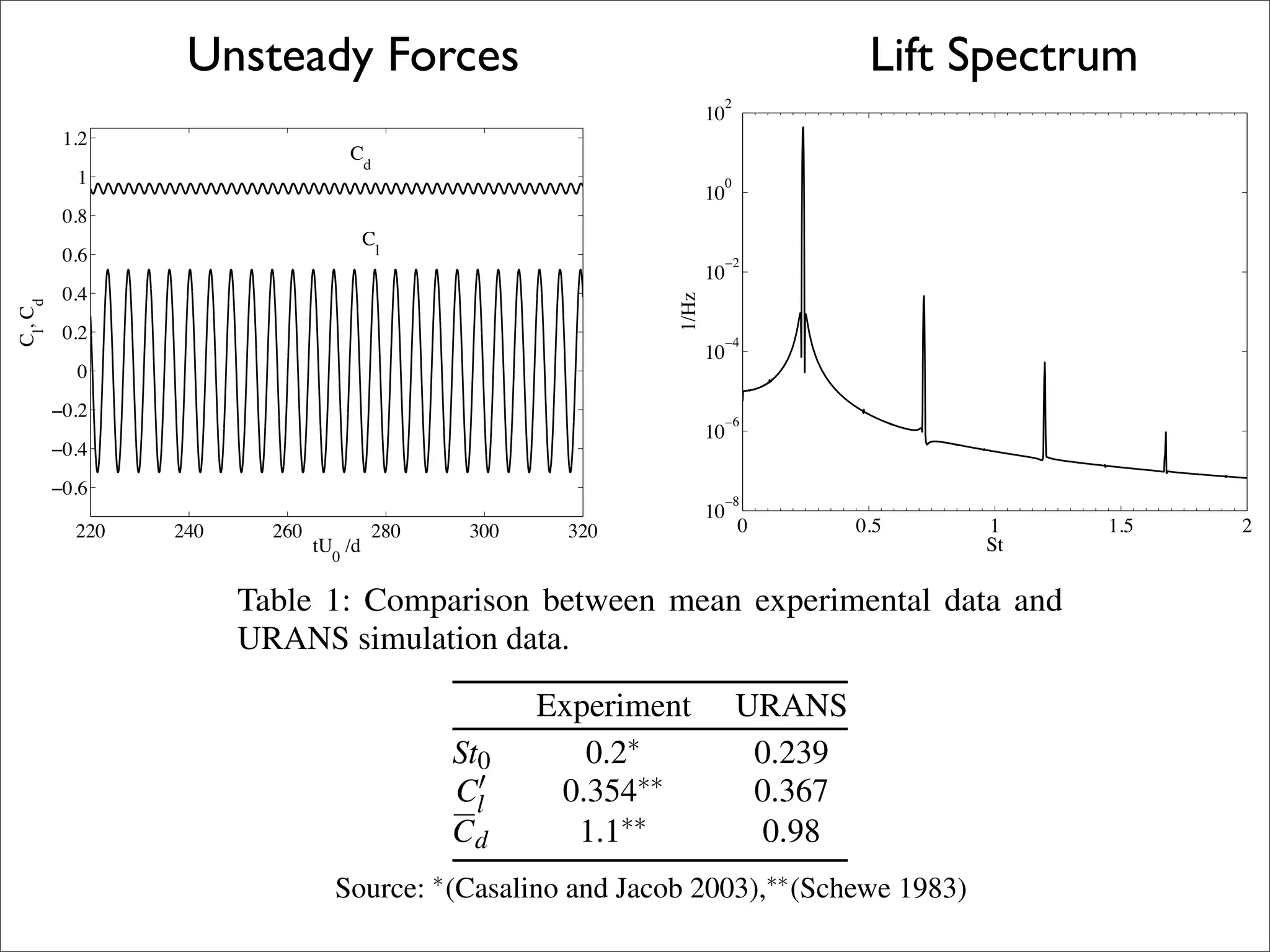
1.2 80
Cd
1 70 With Spanwise Effects
0.8 60 Pure Tone
Cl
0.6
50
PSD [dB/Hz]
0.4
Cl, Cd
40
0.2
30
0
20
−0.2
10
−0.4
−0.6 0
−10
220 240 260 280 300 320 0.1 0.2 0.4 0.8 1 1.4 2
tU0 /d St

13. - is (t) = summarised below.
rue
a normalised time scale associated with the
) using an impulseURANS (t) dτ
h(τ)F response function h(t) (5) This procedure is
e time signal. Australia
009, Adelaide, Note, Gaussian statistics could
0 Temporal Statistics of coherency alon
d. Temporal Model
T way of introducing
nal can be considereddescribed as
sponse function canh(τ)F be as a composite of a
nal simulated a linear distribution a randomly
It URANS (5) flowfield to a noise
Ftrue (t)is signals, each withtrue force F (t) is convoluted over a
=assumed that the(t) dτ
odel calls for 0 of variancetrue simulation.
difference signalφof time length T to the URANS simulated force signal
φτ = τ (τ).
23–25 URANS (t) 2009, be described as(6)
ulse response function can an impulse response
h(t) = e−iφτ using Adelaide, Australia function h(t)
FNovember
To estimate the s
nner as the spatial case (Casalino and Jacob
Using the spanwi
relations (Norberg
ection), (τ is = w
...wτ it t )the true signalthe autocorrelation as a composite measurem
then assumed τt that can be considered
τ,max T (8) phase (φof a
imental η ) is crea
an be number of according τto Laplacian statis-each(6) a randomly
distributed original simulated signals, 3
h(t) = e−iφ (t) = with
Ftrue h(τ)FURANS (t) dτ
instead. (5)
/τc . This variance distribution isφτ = φτ (τ).
dispersed phase difference used to gen-
0 The phase distrib
of phase (φτ ) response τt ≤ 1 that
ispersion If the impulse over 0 ≤ function can be described as time
Frequency Com
In the same manner as the spatial case (Casalino and Jacob
3
τt
arded time of the URANS signal used to cal-
(τ) Autocorrelation function for phase
ρτ2003, see next section), it is assumed that the autocorrelation
q. 4 using = exp − τc (7) The experimental
coefficient (ρτ ) can be distributed according to Laplacian statis- oc
the main tone
−iφτ
, tics h(t) = e URANS simulatio(6)
is the time delayφnormalised by the time base
τ d frequency scaling
is a normalised 2π U0
Time “shift”
Θτ = Θ + time scale associated with (9) the The frequency and
This procedure is
e time signal. Note, Gaussian statistics could τt 3
ρτ (τ) = exp − (7)
of coherency alo
τ

14. 
Spatial Statistics





Proceedings of ACOUSTICS 200

osite of a


randomly |η|
ρ(η) = exp − (12
Ll
and Jacob
Using the spanwise statistical model, a random dispersion i
correlation
phase (φη ) is created along the span of the cylinder.
cian statis- Proceedings of ACOUSTICS 2009
composite of a The phase distribution is then used to
modulate the retarde
with a randomly time ρ(η) = exp −
|η|
(12)
Ll
(7)
alino and Jacob φ d
Using the spanwise statistical + η a random dispersion in
Θη = Θ model, (13
autocorrelation 2π U the
phase (φη ) is created along the span of 0 cylinder.
Laplacian statis-
time base
The phase distribution is then used to modulate the retarded

15. 2D Aerodynamic Simulation
• Circular Cylinder in cross-flow with Re=22,000
• Aim: to simulate noise from turbulent flow interaction,
develop new statistical noise model
• C-Mesh, orthogonal mesh of diameter 16d clearance all
about object, 45,234 cells
• y+ 8, Realisable k-epsilon turbulence model
Full Domain Detail about cylinder

16. 1
Instantaneous Vorticityx/d
0 −0.5
0.5 1 1.5 2 2.5
0.5
1 (a) tU0 /D = 321
0.5 1 (c) tU0 /D = 323
y/d
0.5 0.5
0
y/d
0
y/d
y/d
0 0
−0.5 −0.5
−0.5 −0.5
Figure 4: RMS pres
−1 −1 −1
−1
der in turbulent flow
−0.5 0 0.5 1
x/d
1.5 2 2.5 −0.5 0 0.5 1
x/d
intervals2 ∆prms /(ρ0
1.5 2.5
−0.5 0 0.5 1 1.5
−0.5 2 0 2.50.5 1 1.5 2 2.5
x/d x/d
1 (b) tU0 /D = 322 1 (d) tU0 /D = 324
Figure 4: RMS pres
source associated w
Figure 3: Instantaneous spanwise vorticity in turbulent flow
der contours over on
0.5 0.5 therefore very ineffic
ωz d
vortex shedding cycle. Levels: −15 ≤ U∞ ≤ 15 with intervaU
intervals ∆prms /(ρ0
the surface of the cy
|∆ω|d
y/d
y/d
0
U∞ =5 0
For this case, the uns
−0.5 (b) tU0 /D = 322 −0.5 (d) tU0 /D = 324to noise is that on th
Australian Acoustical Society source associated w
largest unsteady pre
Figure 3: Instantaneous spanwise vorticity contours over o
−1 −1 therefore very ineffic
vortex shedding cycle. Levels: −15 ≤ ωz∞ ≤ 15 withof the c
d
tom surfaces interva
the surface of the cy
1 U 1.5
x/d largest source of noi
−0.5 0 0.5 1 1.5 2 2.5 −0.5 0 0.5 2 2.5
x/d |∆ω|d

17. RMS Pressure
1
0.5
y/d
0
−0.5
−1
−0.5 0 0.5 1 1.5 2 2.5 3
x/d

18. Unsteady Forces Lift Spectrum
2
10
1.2
Cd
1 0
10
0.8
Cl
0.6 −2
10
0.4
1/Hz
Cl, Cd
0.2 −4
10
0
−0.2 −6
10
−0.4
−0.6
−8
10
220 240 260 280 300 320 0 0.5 1 1.5 2
tU0 /d 23–25 November 2009, Adelaide, Australia
St
Table 1: Comparison between mean experimental data and
URANS simulation data.
Experiment URANS
St0 0.2∗ 0.239
Cl 0.354∗∗ 0.367
Cd 1.1∗∗ 0.98
Source: ∗ (Casalino and Jacob 2003),∗∗ (Schewe 1983)

19. Time Series Acoustic Pressure
−4
x 10
1
0.5
2
p /ρU0
0
ʹ′
−0.5
−1
0 50 100 150 200 250 300 350 400
tU /D
0
Assumed characteristic time ~60 vortex shedding periods
and spanwise correlation length of 0.27 x span.

20. Acoustic PSD at 86.25D above centre of cylinder
80
URANS + Statistics
70
URANS
60 Experiment
50
PSD [dB/Hz]
40
30
20
10
0
0.1 0.2 0.4 0.8 1 1.4 2
St
100 statistical acoustic signal PSD’s were averaged.

21. Application to the NASA Tandem Cylinder Case
120
URANS + Statistics
110
2D URANS
100 Experiment (NASA QFF)
90
PSD [dB/Hz]
80
70
60
50
40
0.1 0.2 0.4 0.8 1 1.4 2
St
Grid Acoustics
1.5 15
1
Flow: vorticity 10
0.5 5
y/d
0 0
−0.5 −5
−1 −10
−1.5 −15
−1 0 1 2 3 4 5 6
x/d

22. Conclusions
• A methodology for correcting URANS CFD
data to appropriate noise source terms has
been presented
• When applied to cylinder flows, the method
correctly recreates the spectral broadening
about the main tone
• At this stage, the method has difficulty in
recreating the harmonics